On Transmit Beamforming for MISO-OFDM Channels With Finite-Rate Feedback

Abstract

With finite-rate feedback, we propose two feedback methods for transmit beamforming in a point-to-point MISO-OFDM channel. For the first method, a receiver with perfect channel information, quantizes and feeds back the optimal transmit beamforming vectors of a few selected subcarriers, which are equally spaced. Based on those quantized vectors, the transmitter applies either constant, linear, or higher-order interpolation with the remaining beamforming vectors. With constant interpolation, we derive the approximate sum achievable rate and the optimal cluster size that maximizes the approximate rate. For linear interpolation, we derive a closed-form expression for the phase rotation by utilizing the correlation between OFDM subcarriers. We also propose a higher-order interpolation that requires more than two quantized vectors to interpolate transmit beamformers, and is based on existing channel estimation methods. Numerical results show that interpolation with the optimized cluster size can perform significantly better than that with an arbitrary cluster size. For the second proposed method, a channel impulse response is quantized with a uniform scalar quantizer. With channel quantization, we also derive the approximate sum achievable rate. We show that switching between the two methods for different feedback-rate requirements can perform better than the existing schemes.

I Introduction

Equipping a transmitter and/or a receiver with multiple antennas creates a multiantenna wireless channel whose capacity depends on the channel information available at the transmitter and/or receiver. In multiantenna channels, transmit beamforming has been shown to increase an achievable rate by directing transmit signal toward the strongest channel mode [1]. With channel information, the receiver can compute the optimal beamforming vector that maximizes achievable rate and feeds the vector back to the transmitter. Due to a finite feedback rate, the beamforming vector needs to be quantized. Several quantization schemes and codebooks have been proposed and analyzed, and the corresponding performance was shown to depend on the codebook design and the number of available feedback bits [2, 3, see references therein]. In this work, we consider transmit beamforming for multiple-input single-output (MISO) orthogonal frequency-division multiplexing (OFDM).

In MISO-OFDM, a wideband channel is converted into parallel narrowband subchannels. For each subchannel or subcarrier, the optimal beamforming vector is different and needs to be quantized at the receiver and fed back to the transmitter. The total number of feedback bits required increases with the number of subcarriers, which can be large. References [4, 5, 6, 7, 8, 9, 10, 11, 12, 13, 14, 15, 16, 17, 18] have proposed to reduce the amount of feedback while maintaining performance. Due to high channel correlation in time and frequency domains, feedback of transmit precoding matrices across time and subcarriers can be compressed. References [16, 17] proposed to compress feedback with either recursive or trellis-based encodings.

In [4, 9, 15, 18], the optimal transmit beamforming vectors of selected subcarriers, which are a few subcarriers apart, are quantized while the remaining ones are approximated to equal the quantized vector of the closest subcarrier. The remaining transmit beamforming vectors are proposed to be linearly interpolated in [5, 12] and spherically interpolated in [6, 13, 11]. In [10], the authors proposed to quantize the averaged optimal transmit beamformer in each cluster termed mean clustering. Geodesic-based interpolation of transmit precoding matrices was also proposed in [10] and was extended to multiuser channels in [14]. In [8], each subcarrier cluster uses the same beamforming vector or precoding matrix, which is searched from a subcodebook that contains entries close to the beamformer or precoder in the adjacent cluster. Hence, there is some saving in feedback bits. Most of the works mentioned proposed to use either the same or interpolated beamforming vectors for a group or cluster of adjacent subcarriers since subcarriers are highly correlated in a frequency-selective channel. However, none has analyzed the optimal cluster size and the associated performance.

Given a limited feedback rate, we propose to quantize the optimal beamforming vector at every few subcarriers with the random vector quantization (RVQ) codebook proposed by [2] and to either use the same quantized vector for the whole subcarrier cluster or interpolate the remaining beamforming vectors in the cluster from the quantized vectors. For the first proposed method termed constant interpolation, we derive an approximate sum achievable rate over all subcarriers. The analytical approximation can predict the performance trend well and the optimal cluster size accurately. The optimal cluster size depends mainly on the available feedback rate, and on how frequency-selective the current channel is.

For linear interpolation, we propose a closed-form expression for the phase-rotation parameter based on the correlation between the transmit beamformers of subcarriers in the cluster. In earlier work by [5], the parameter was exhaustively searched. Our modified linear interpolation requires fewer minimum feedback bits than that in [5]. In [12], the expression for the phase-rotation parameter was also proposed and is based on a chordal distance between two quantized beamforming vectors of the adjacent clusters. However, our proposed phase rotation combined with the optimized cluster size outperforms the phase rotation proposed by [12].

For higher-order interpolation, our method is based on earlier works on comb-type pilot based channel estimation in OFDM [19, 20, 21]. Three or more quantized beamforming vectors from adjacent clusters are used to interpolate all beamforming vectors in one cluster. The number of phase-rotation parameters increases with the order of the interpolation. The set of phase-rotation parameters that maximizes sum achievable rate in a cluster can be searched from the codebook proposed by [5]. Reference [6] modified the second-order channel estimation in [21] to interpolate transmit beamforming vectors for subcarriers in a multiple-input multiple-output (MIMO)-OFDM channel. In [13] the authors based their method from the work by [19] to interpolate transmit beamformers for subcarriers, but without phase rotations. The lack of phase-rotation parameters degrades significantly the performance of the method in [13]. Our numerical example shows that the higher-order interpolation with our optimized cluster size results in a good performance in a high feedback-rate regime.

When the feedback rate is high, we propose to quantize the channel impulse response with a uniform scalar quantizer and derive the approximate sum rate for MISO channels. The scalar quantization used in the proposed method is less complex than the vector quantization used in [7]. The proposed scalar quantization of the channel impulse response is shown to perform well with a high feedback rate. Similar results were observed by [2] where the optimal beamformer and not the channel response was scalar quantized. We note that [22] also proposed to scalar quantize a channel impulse response, but the resulting sum rate was not analyzed.

Apart from what was presented earlier in [23, 24], here we show details of all proofs and update the derivation of the achievable rate approximation in Proposition 1. We compare our proposed feedback methods with several existing ones in the literature and show that selecting the optimal cluster size that maximizes the sum rate can significantly improve the sum rate. Higher-order interpolation with quantized transmit beamforming is also proposed.

This paper is organized as follows. Section II describes channel and feedback models as well as formulates the finite feedback-rate problem. We propose beamforming interpolation methods and analyze the optimal cluster size in Section III. Direct quantization of channel impulse response and its performance analysis are shown in Section IV. Numerical results and conclusions are in Sections V and VI, respectively. Finally, all proofs are in appendices.

II System Model

We consider a point-to-point, discrete-time, MISO-OFDM channel with $N$ subcarriers. A transmitter is equipped with $N_{t}$ antennas while a receiver is equipped with a single antenna. We assume that the transmit antennas are placed sufficiently far apart that they are independent. For each transmit-receive antenna pair, a transmitted signal propagates through a frequency-selective Rayleigh fading channel with order $L$. Applying a discrete Fourier transform (DFT), the frequency response for the $n$th subcarrier and the $n_{t}$th transmit antenna is given by

$$h_{n,n_{t}}=\sum_{l=0}^{L-1}g_{l,n_{t}}\mathrm{e}^{\frac{-j2\pi ln}{N}}$$ (1)

where $g_{l,n_{t}}$ is a complex channel gain for the $l$th path between the $n_{t}$th transmit and receive antenna pairs. Assuming a rich scattering, $g_{l,n_{t}}$ for all $L$ paths and all $N_{t}$ transmit antennas are independent complex Gaussian distributed with zero mean and variance $E|g_{l,n_{t}}|^{2}$. In this work, we assume a uniform power delay profile for which the power of each path is the same and the total channel power for each transmit-receive antenna pair is one. Hence, $E|g_{l,n_{t}}|^{2}=\frac{1}{L}$. Let $\bm{h}_{n}$ denote an $N_{t}\times 1$ channel vector of the $n$th subcarrier, whose entry is $h_{n,n_{t}}$ shown in (1). Thus,

$$\bm{h}_{n}=\left[h_{n,1}\quad h_{n,2}\ \cdots\ h_{n,N_{t}}\right]^{T}.$$ (2)

Assuming a transmit beamforming or a rank-one precoding, the received signal on the $n$th subcarrier is given by

$$r_{n}=\bm{h}_{n}^{{\dagger}}\bm{v}_{n}x_{n}+z_{n},\quad 1\leq n\leq N,$$ (3)

where $\bm{v}_{n}$ is an $N_{t}\times 1$ unit-norm beamforming vector, $x_{n}$ is a transmitted symbol with zero mean and unit variance, and $z_{n}$ is an additive white Gaussian noise with zero mean and variance $\sigma^{2}_{z}$. With perfect channel information at the transmitter, the optimal transmit precoding that maximizes an achievable rate for MISO channel is rank-one. This fact motivates us to use a rank-one precoding or beamforming. A resulting sum achievable rate over $N$ subcarriers is given by

$$C=\sum_{n=1}^{N}E\left[\log(1+\rho|\bm{h}_{n}^{{\dagger}}\bm{v}_{n}|^{2})\right]$$ (4)

where the expectation is over the distribution of $\bm{h}_{n}$. We assume a uniform power allocation for all subcarriers and hence, the background signal-to-noise ratio (SNR) for each subcarrier $\rho=1/\sigma^{2}_{z}$.

From (4), we note that the sum achievable rate is a function of transmit beamforming vectors $\{\bm{v}_{1},\bm{v}_{2},\ldots,\bm{v}_{N}\}$. A receiver with perfect channel information can optimize the sum achievable rate over the transmit beamforming vectors and send the selected beamforming vectors to the transmitter via a feedback channel. Since the feedback channel between the receiver and the transmitter has a finite rate, quantizing the transmit beamforming vectors is required. In this study we apply a random vector quantization (RVQ) codebook whose entries are independent, isotropically distributed vectors to quantize a transmit beamforming vector. RVQ is simple, however has been shown to perform close to the optimum codebook [2, 25].

We assume $B$ total feedback bits per update. For an equal-bit-per-subcarrier allocation, each beamforming vector is quantized with $B/N$ bits. Let us denote the RVQ codebook by $\mathcal{V}=\{\bm{w}_{1},\bm{w}_{2},\ldots,\bm{w}_{2^{B/N}}\}$ with $2^{B/N}$ entries. The receiver selects for the $n$th subcarrier the entry in the codebook that maximizes an instantaneous achievable rate as follows:

$$\hat{\bm{v}}_{n} =\arg\max_{\bm{w}\in\mathcal{V}}\ \log(1+\rho|\bm{h}_{n}^{{\dagger}}\bm{w}|^{2})$$ (5)

$$=\arg\max_{\bm{w}\in\mathcal{V}}\ |\bm{h}_{n}^{{\dagger}}\bm{w}|^{2}$$ (6)

and the associated achievable rate for the $n$th subcarrier is given by

$$C_{n} =E\left[\log(1+\rho|\bm{h}_{n}^{{\dagger}}\hat{\bm{v}}_{n}|^{2})\right]$$ (7)

$$=E\left[\log(1+\rho\|\bm{h}_{n}\|^{2}|\bar{\bm{h}}_{n}^{{\dagger}}\hat{\bm{v}}_{n}|^{2})\right].$$ (8)

where $\bar{\bm{h}}_{n}=\bm{h}_{n}/\|\bm{h}_{n}\|$ is a unit-norm channel vector that points in the same direction as $\bm{h}_{n}$. Evaluating (8) was shown by [25]. We note from (8) that the achievable rate depends on the number of feedback bits per subcarrier, which could be small due to a large number of subcarriers in a practical OFDM system. Hence, this may result in a large quantization error, which leads to a substantial performance loss.

III Interpolating Transmit Beamforming Vectors

Feeding back transmit beamforming vectors of all subcarriers requires quantizing $NN_{t}$ complex coefficients and thus, a large number of feedback bits. We note that adjacent subcarriers in OFDM are highly correlated since the number of channel taps is much lower than that of subcarriers ($L\ll N$). The optimal transmit beamformers, which depend on channel matrices, are also highly correlated. In this section, we propose beamforming interpolation of different orders to reduce the number of feedback bits while maintaining the performance.

First we evaluate a squared correlation between normalized channel vectors of subcarrier $n$ and $n+q$ defined by

$$E\left[|\bar{\bm{h}}_{n}^{{\dagger}}\bar{\bm{h}}_{n+q}|^{2}\right]=E\left[\frac{|\bm{h}_{n}^{{\dagger}}\bm{h}_{n+q}|^{2}}{\|\bm{h}_{n}\|^{2}\|\bm{h}_{n+q}\|^{2}}\right].$$ (9)

Evaluating (9) is not tractable for a finite-size system. Hence, we approximate the average squared correlation as follows.

Lemma 1

A squared correlation between the $n$th and $n+q$th normalized channel vectors is approximated as follows:

$$E\left[|\bar{\bm{h}}_{n}^{{\dagger}}\bar{\bm{h}}_{n+q}|^{2}\right] \approx\frac{L^{2}+N_{t}\varphi^{2}(q)}{L^{2}N_{t}+\varphi^{2}(q)}$$ (10)

$$\triangleq\psi(q,N_{t})$$ (11)

where

$$\varphi(x)=\frac{\sin(\frac{\pi xL}{N})}{\sin(\frac{\pi x}{N})}.$$ (12)

The proof of Lemma 1 is shown in Appendix -A.

As subsequent numerical example in Section V will show that approximation in Lemma 1 closely predicts the result of a finite-size system. The correlation in (10) depends on $L$, $N$, $N_{t}$, and most importantly, $q$, which indicates how far apart the two channel vectors are. When $q\to 0$, $\varphi(q)\to L$ and the squared correlation becomes $\|\bar{\bm{h}}_{n}\|^{4}\to 1$. We note that the number of channel taps $L$ and channel impulse response can be accurately estimated as shown in [26].

III-A Constant Interpolation

In the first method, we group adjacent contiguous subcarriers into a cluster and apply the same quantized beamforming vector for all subcarriers in the cluster. We denote the number of contiguous subcarriers in one cluster by $M$. Thus, the number of clusters is given by $K\triangleq\lfloor N/M\rfloor$ with a possible few remaining subcarriers. The number of feedback bits allocated for each cluster is equal to $B/K$. All $B/K$ bits are used to quantize the beamforming vector of the centered subcarrier for odd $M$ and one subcarrier off the center for even $M$. Therefore, the beamforming vector used for the $k$th cluster is given by

$$\hat{\bm{v}}_{kM+m}=\left\{\begin{array}[]{lr}\arg\max_{\bm{w}\in\mathcal{V}}\ |\bar{\bm{h}}_{kM+\frac{M+1}{2}}^{{\dagger}}\bm{w}|^{2}&\text{for odd}\ M\\ \arg\max_{\bm{w}\in\mathcal{V}}\ |\bar{\bm{h}}_{kM+\frac{M}{2}}^{{\dagger}}\bm{w}|^{2}&\text{for even}\ M\end{array}\right.$$ (13)

where $1\leq m\leq M$ and $0\leq k\leq K-1$. If $N/M$ is not an integer, then there exist some remaining subcarriers, which do not belong in any cluster. We propose to set the transmit beamforming for these subcarriers to be that of the last cluster as follows:

$$\hat{\bm{v}}_{KM+q}=\hat{\bm{v}}_{KM}\quad\text{for}\ 1\leq q\leq N-KM.$$ (14)

With constant interpolation, an achievable rate for each subcarrier can be approximated by Proposition 1 .

Proposition 1

For $1\leq n+q\leq N$, the approximate ergodic achievable rate of the $(n+q)$th subcarrier is given by

$$C_{n+q}\approx\mathsf{C}_{n+q}=\log(1+\rho N_{t}\gamma(n+q,B/K))$$ (15)

where

$$\gamma(n+q,B/K)\triangleq\psi(q,N_{t})\cdot(1-2^{B/K}\beta(2^{B/K},\frac{N_{t}}{N_{t}-1}))\\ +(1-\psi(q,N_{t}))\cdot\frac{(2^{B/K}\beta(2^{B/K},\frac{N_{t}}{N_{t}-1}))}{N_{t}-1}$$ (16)

and the beta function $\beta(x,y)=\int_{0}^{1}t^{x-1}(1-t)^{y-1}\,\mathrm{d}t$.

The proof of Proposition 1 is shown in Appendix -B.

With Proposition 1, we obtain the approximate sum achievable rate for a single cluster with odd $M$ as follows:

$$\mathsf{C}_{\text{cluster}}=\sum_{q=-\frac{M-1}{2}}^{\frac{M-1}{2}}\mathsf{C}_{n+q}=\log(1+\rho N_{t}\gamma(0,B/K))\\ +2\sum_{q=1}^{\frac{M-1}{2}}\log(1+\rho N_{t}\gamma(q,B/K)).$$ (17)

With even $M$, the sum achievable rate for a single cluster is approximated by

$$\mathsf{C}_{\text{cluster}}=\log(1+\rho N_{t}\gamma(0,B/K))\\ +2\sum_{q=1}^{\frac{M}{2}-1}\log(1+\rho N_{t}\gamma(q,B/K))+\log(1+\rho N_{t}\gamma(\frac{M}{2},B/K)).$$ (18)

We note that the performance of the constant interpolation has a trade-off between total feedback bits and cluster size and hence, there exists optimal cluster size for a given feedback budget. Given $B$ feedback bits and other system parameters, we would like to determine the number of subcarriers $M^{*}$, which maximizes the approximate sum achievable rate of all $N$ subcarriers given by

$$M^{*}=\arg\max_{\begin{subarray}{c}1\leq M\leq N\\ M\in\mathbb{Z}\end{subarray}}\Bigg{\{}K\mathsf{C}_{\text{cluster}}\\ +\sum_{r=1}^{N-KM}\log(1+\rho N_{t}\gamma(r+\frac{M}{2},B/K))\Bigg{\}}$$ (19)

where the first term accounts for the approximate achievable rate of the $K$ clusters and the second term accounts for the approximate achievable rate of a few remaining subcarriers. Solving (19) can be accomplished by either integer programming for which there exist many available tools or by exhaustive search. Although the optimization in (19) is based on the approximation of the actual achievable rate, subsequent numerical examples in Section V show that the solution to (19) accurately predicts the optimal cluster size. We note that there is no other comparable analysis on the optimal cluster size in the literature.

Besides the sum achievable rate, another important performance metric is the average received power across subcarriers defined as follows:

$$\eta_{\text{AVE}} \triangleq\frac{1}{N}\sum_{n=1}^{N}\rho E\left[|\bm{h}_{n}^{{\dagger}}\hat{\bm{v}}_{n}|^{2}\right]$$ (20)

$$=\frac{\rho N_{t}}{N}\sum_{n=1}^{N}E\left[|\bar{\bm{h}}_{n}^{\dagger}\hat{\bm{v}}_{n}|^{2}\right].$$ (21)

where it is shown in the proof of Proposition 1 that

$$E\left[|\bar{\bm{h}}_{n}^{\dagger}\hat{\bm{v}}_{n}|^{2}\right]\approx\gamma(n,B/K).$$ (22)

Therefore, the average received power can be approximated as follows.

Corollary 1

For odd $M$,

$$\eta_{\text{AVE}}\approx\frac{\rho N_{t}}{N}\Bigg{\{}K\gamma(0,B/K)+2K\sum_{q=1}^{\frac{M-1}{2}}\gamma(q,B/K)\\ +\sum_{r=1}^{N-KM}\gamma(r+\frac{M}{2},B/K)\Bigg{\}},$$ (23)

and for even $M$

$$\eta_{\text{AVE}}\approx\frac{\rho N_{t}}{N}\Bigg{\{}K\gamma(0,B/K)+2K\sum_{q=1}^{\frac{M}{2}-1}\rho\gamma(q,B/K)\\ +K\gamma(\frac{M}{2},B/K)+\sum_{r=1}^{N-KM}\gamma(r+\frac{M}{2},B/K)\Bigg{\}}.$$ (24)

These analytical expressions give a more accurate approximation than those in Proposition 1 since there is no Jensen’s inequality involved as demonstrated by numerical results in Section V.

III-B Linear Interpolation

To increase the performance, we propose to modify a linear interpolation proposed by [5]. Similar to the constant interpolation, all subcarriers are grouped into $K$ clusters. Each cluster consists of $M$ contiguous subcarriers and a possible last cluster with a few remaining subcarriers. For each cluster, the optimal beamforming vector of the first subcarrier is selected from an RVQ codebook with either $B/K$ bits or $B/(K+1)$ bits, depending on the total number of clusters.

All other beamforming vectors in a cluster are linear combinations of the quantized beamforming vector of the first subcarrier in the cluster and that in the next cluster as follows [5]:

$$\hat{\bm{v}}_{kM+m}(\theta_{m})\triangleq\frac{(1-c_{m})\hat{\bm{v}}_{kM}+c_{m}\mathrm{e}^{j\theta_{m}}\hat{\bm{v}}_{(k+1)M}}{\|(1-c_{m})\hat{\bm{v}}_{kM}+c_{m}\mathrm{e}^{j\theta_{m}}\hat{\bm{v}}_{(k+1)M}\|}$$ (25)

for $1\leq m\leq M-1$ and $0\leq k\leq K-1$, where

$$c_{m}=\frac{m}{M}$$ (26)

is a linear weight and $\theta_{m}$ is a phase-rotation parameter. We note that for the last cluster, we choose to interpolate with $\hat{\bm{v}}_{1}$ instead of $\hat{\bm{v}}_{N}$ to save some feedback bits. Due to DFT, $\bar{\bm{h}}_{1}$ is similar to $\bar{\bm{h}}_{N}$ and hence, $\hat{\bm{v}}_{1}$ is also similar to $\hat{\bm{v}}_{N}$.

In [5], $\theta_{m}$ is chosen to maximize the sum achievable rate in (4) by performing exhaustive search over the received power in each cluster as follows. For the $k$th cluster,

$$\theta_{m}=\arg\max_{\theta\in\Theta}\sum_{i=1}^{M}|\bm{h}_{kM+i}^{{\dagger}}\hat{\bm{v}}_{kM+i}(\theta)|^{2}$$ (27)

where the phase-rotation codebook

$$\Theta=\left\{0,2\pi\frac{1}{P},2\pi\frac{2}{P}\ldots,2\pi\frac{P-1}{P}\right\}$$ (28)

and $P$ is the number of quantization levels.

To avoid search complexity and reduce feedback, here we propose to determine the phase rotation based on a correlation between the optimal beamformers of neighboring subcarriers. We note that the optimal transmit beamforming vector for the $n$th subcarrier is matched to the normalized channel vector $\bm{v}_{n}^{\mathrm{opt}}=\bar{\bm{h}}_{n}$. Evaluating a correlation between the optimal beamformer and the interpolated beamformer that are $m$ subcarriers apart, $E|(\bm{v}_{kM}^{\mathrm{opt}})^{{\dagger}}\bm{v}_{kM+m}|^{2}$, follows similar steps to the proof of Lemma 1. This correlation is most likely close to the correlation between the optimal beamformers, which is approximated to be $\psi(m,N_{t})$ in (11). Based on this assumption, we set $E|(\bm{v}_{kM}^{\mathrm{opt}})^{{\dagger}}\bm{v}_{kM+m}|^{2}$ to $\psi(m,N_{t})$ and solve for the phase-rotation parameter given by the following proposition.

Proposition 2

The phase rotation for the $m$th subcarrier in the cluster is given by

$$\theta_{m}=\arccos\frac{U(m)}{V(m)}$$ (29)

where

$$U(m)=(1-c_{m})^{2}(\psi(m,N_{t})-N_{t}+1)\\ +c_{m}^{2}(N_{t}\psi(m,N_{t})-\frac{N_{t}}{L^{2}}\varphi^{2}(M)+1)$$ (30)

and

$$V(m)=\frac{2}{L}(1-c_{m})c_{m}(N_{t}-N_{t}\psi(m,N_{t})+1)\\ \cdot\varphi(M)\cos\left(\frac{\pi M(L-1)}{N}\right).$$ (31)

The proof is shown in Appendix -C.

Finding the optimal cluster size for the linear interpolation is not tractable since the achievable rate expression is not known. From numerical results, the optimal cluster of the constant interpolation mostly aligns with that of the linear interpolation and that of higher-order interpolations as well. We note that computing $\theta_{m}$ in Proposition 2 can be performed at the transmitter with the number of channel taps $L$ and cluster size $M$. For a relatively static environment, $L$ and hence $M$ may not change often [27]. Thus, feedback for these parameters do not occur often and consists of minimal number of bits. For [5], the phase-rotation needs to be fed back for every cluster. The number of additional feedback bits in [5] increases linearly with the number of clusters and can be significantly larger than that in our method.

III-C Higher-Order Interpolation

For a better interpolation, more than two quantized transmit beamforming vectors should be used to interpolate the beamforming vectors in the cluster. For instance, the second-order interpolated transmit beamformer in the $k$th cluster is as follows:

$$\hat{\bm{v}}_{kM+m}\\ =\frac{\alpha_{-1}\mathrm{e}^{j\theta_{m;-1}}\hat{\bm{v}}_{(k-1)M}+\alpha_{0}\hat{\bm{v}}_{kM}+\alpha_{1}\mathrm{e}^{j\theta_{m;1}}\hat{\bm{v}}_{(k+1)M}}{\|\alpha_{-1}\mathrm{e}^{j\theta_{m;-1}}\hat{\bm{v}}_{(k-1)M}+\alpha_{0}\hat{\bm{v}}_{kM}+\alpha_{1}\mathrm{e}^{j\theta_{m;1}}\hat{\bm{v}}_{(k+1)M}\|}.$$ (32)

We note that there are 3 quantized beamformers $\hat{\bm{v}}_{(k-1)M},\hat{\bm{v}}_{kM},\hat{\bm{v}}_{(k+1)M}$, which are used for interpolation. This interpolation was modified from the channel interpolation methods proposed by [20, 19]. The set of constants is given by [19]

$$\alpha_{-1}=\frac{1}{2}c_{m}(c_{m}-1)$$ (33)

$$\alpha_{0}=-(c_{m}-1)(c_{m}+1)$$ (34)

$$\alpha_{1}=\frac{1}{2}c_{m}(c_{m}+1).$$ (35)

Phase-rotation parameters $\theta_{m;-1}$ and $\theta_{m;1}$ are introduced in this study to increase the performance of the higher-order interpolation. Similar to that in the linear interpolation, the set of the two phase rotations is found by maximizing the sum received power in the $k$th cluster over the codebook $\Theta$ as follows:

$$\max_{\{\theta_{m;-1},\theta_{m;1}\}\in\Theta^{2}}\sum_{i=1}^{M}|\bm{h}_{kM+i}^{{\dagger}}\hat{\bm{v}}_{kM+i}|^{2}.$$ (36)

For order $R$ where $R$ is even and $R>2$, the interpolated beamformer in the $k$th cluster is given by

$$\hat{\bm{v}}_{kM+m}=\frac{\bf{y}}{\|\bf{y}\|}$$ (37)

where

$${\bf{y}}=\sum_{s=-\frac{R}{2}}^{-1}\alpha_{s}\mathrm{e}^{j\theta_{m;s}}\hat{\bm{v}}_{(k+s)M}\\ +\alpha_{0}\hat{\bm{v}}_{kM}+\sum_{t=1}^{\frac{R}{2}}\alpha_{t}\mathrm{e}^{j\theta_{m;t}}\hat{\bm{v}}_{(k+t)M}$$ (38)

and $\{\alpha_{r}\}_{r=-\frac{R}{2}}^{\frac{R}{2}}$ is a set of interpolation constants while the set of phase rotations

$$\{\theta_{m;-\frac{R}{2}},\ldots,\theta_{m;-1},\theta_{m;1},\ldots,\theta_{m;\frac{R}{2}}\}$$

can be found by exhaustive search over the phase codebook $\Theta$.

We expect the higher-order interpolation method to perform better than the previous methods, but the performance gain is obtained at the expense of additional complexity and feedback. Search complexity to locate the optimal set of phase-rotation parameters increases with the number of phase rotations or the order of the interpolation. Also, the additional number of feedback bits to quantize these phase rotations increases with the number of clusters and the order of the interpolation. These bits are in addition to the number of bits used to quantize transmit beamformers.

IV Quantizing Channel Impulse Response

When the available feedback rate is sufficiently high (larger than 2 bits per complex entry), quantizing the channel impulse response directly can perform well [28]. Here we propose to quantize all channel taps of all transmit-receive antenna pairs with a scalar uniform quantizer. A uniform quantizer is simple and performs close to the optimal quantizer when the number of quantization bits is high. Real and imaginary parts of all channel taps are quantized independently with the same number of bits, which is $\frac{B}{2N_{t}L}$. Thus, the quantized $l$th channel tap for the $n_{t}$th transmit-receive antenna pair is given by

$$\hat{g}_{l,n_{t}} =\hat{g}_{l,n_{t},r}+j\hat{g}_{l,n_{t},i}$$ (39)

$$=Q(g_{l,n_{t},r})+jQ(g_{l,n_{t},i})$$ (40)

where $g_{l,n_{t},r}$ and $g_{l,n_{t},i}$ are real and imaginary parts of $g_{l,n_{t}}$, respectively, $Q(\cdot)$ is the uniform scalar quantizer with $2^{\frac{B}{2N_{t}L}}$ steps, while variables with hats denote outputs of the quantizer. Here we select a step size of the quantizer by the existing rule of thumb for Gaussian input (cf. [29, p. 125])

$$\Delta=\frac{4E[(g_{l,n_{t},r})^{2}]}{2^{\frac{B}{2N_{t}L}}}=\frac{1}{\sqrt{L}}2^{\frac{3}{2}-\frac{B}{2N_{t}L}},$$ (41)

which changes with the variance of the channel tap and the number of quantization bits. Then, the transmitter computes a DFT of the quantized channel impulse response to obtain an approximate frequency response as follows:

$$\hat{h}_{n,n_{t}}=\sum_{l=0}^{L-1}\hat{g}_{l,n_{t}}\mathrm{e}^{-\frac{j2\pi ln}{N}},$$ (42)

which is the $n_{t}$th entry of the quantized $N_{t}\times 1$ channel vector for the $n$th subcarrier denoted by $\hat{\bm{h}}_{n}=\left[\hat{h}_{n,1}\quad\hat{h}_{n,2}\ \cdots\ \hat{h}_{n,N_{t}}\right]^{T}$.

Based on $\hat{\bm{h}}_{n}$, the transmitter transmits signal in the direction of the quantized channel vector, namely, $\hat{\bm{h}}_{n}/\|\hat{\bm{h}}_{n}\|$ and the corresponding sum rate over all subcarriers is given by

$$C =\sum_{n=1}^{N}E\left[\log(1+\rho\frac{|\bm{h}_{n}^{\dagger}\hat{\bm{h}}_{n}|^{2}}{\|\hat{\bm{h}}_{n}\|^{2}})\right]$$ (43)

$$=NE\left[\log(1+\rho\frac{|\bm{h}_{n}^{\dagger}\hat{\bm{h}}_{n}|^{2}}{\|\hat{\bm{h}}_{n}\|^{2}})\right]$$ (44)

$$\leq N\log(1+\rho E\left[\frac{|\bm{h}_{n}^{\dagger}\hat{\bm{h}}_{n}|^{2}}{\|\hat{\bm{h}}_{n}\|^{2}}\right])$$ (45)

$$\approx N\log(1+\rho\frac{E[|\bm{h}_{n}^{\dagger}\hat{\bm{h}}_{n}|^{2}]}{E[\|\hat{\bm{h}}_{n}\|^{2}]})$$ (46)

where in (44), we use the fact that the distribution of subcarriers is identical and in (45) and (46), we apply Jensen’s inequality and approximate an expectation of the quotient by a quotient of the two expectations. The approximation becomes more accurate as the number of transmit antennas increases [30]. Consequently, we obtain the approximate sum achievable rate.

Since real and imaginary parts of each channel tap are independent and Gaussian distributed with zero mean and variance $\frac{1}{2L}$, we can easily show that

$$E[\|\hat{\bm{h}}_{n}\|^{2}]=N_{t}(1-2LE[(\hat{g}_{r}-g_{r})^{2}])$$ (47)

and

$$\begin{split}E[|\bm{h}_{n}\hat{\bm{h}}_{n}^{\dagger}|^{2}]=N_{t}(&1+\frac{1}{L}-(2L-1)E[(\hat{g}_{r}-g_{r})^{2}]\\ &+2LE[\hat{g}_{r}^{2}g_{r}^{2}]+4L(N_{t}L-1)E^{2}[\hat{g}_{r}g_{r}])\end{split}$$ (48)

where we have dropped indices $n_{t}$ and $l$ from $g_{l,n_{t},r}$ for clarity. The mean squared error is given by

$$E[(\hat{g}_{r}-g_{r})^{2}]=\int(Q(x)-x)^{2}f_{g_{r}}(x)\,\mathrm{d}x$$ (49)

and the correlation and its second moment are given by

$$E[\hat{g}_{r}g_{r}]=\int xQ(x)f_{g_{r}}(x)\,\mathrm{d}x$$ (50)

$$E[\hat{g}_{r}^{2}g_{r}^{2}]=\int x^{2}Q^{2}(x)f_{g_{r}}(x)\,\mathrm{d}x.$$ (51)

where $f_{g_{r}}(\cdot)$ denotes the probability density function (pdf) of $g_{l,n_{t},r}$.

Each term in (49)-(51) can be computed numerically. However, to obtain some insight on how the sum achievable rate depends on the feedback rate and other channel parameters, we approximate each term in a high feedback-rate regime. It was shown that for large $B$ [31],

$$E[(\hat{g}_{r}-g_{r})^{2}]\approx\frac{\Delta^{2}}{12}=\frac{2}{3L}2^{-\frac{B}{N_{t}L}}.$$ (52)

Applying the property of the optimum quantizer [32], we obtain

$$E[\hat{g}_{r}g_{r}]\approx\frac{1}{2L}-E[(\hat{g}_{r}-g_{r})^{2}].$$ (53)

As $B\to\infty$, $\hat{g}_{r}\to g_{r}$. Hence,

$$\lim_{B\to\infty}E[\hat{g}_{r}^{2}g_{r}^{2}]=\frac{3}{4L^{2}}.$$ (54)

Substituting (52) – (54) into (47) and (48), we obtain the approximate upper bound for a sum achievable rate for the MISO channel with large $B$ as follows

$$C\approx N\log(1+\rho(1-\frac{1}{L}+(N_{t}L-1)\Omega_{B}+\frac{3}{4L^{2}\Omega_{B}}))$$ (55)

where $\Omega_{B}=\frac{1}{L}-\frac{4}{3L}2^{-\frac{B}{N_{t}L}}$. As the number of feedback bits per transmit antenna and channel tap, $\frac{B}{N_{t}L}$, increases, the quantization error (52) decreases and the sum rate (55) increases. We note that for as $\frac{B}{N_{t}L}\to\infty$ and $N_{t}$ increases, the sum rate in (55) increases as $N\log(\rho N_{t})$, which is the sum rate with perfect CSI. With a large feedback rate, quantizing channel impulse response can achieve a larger sum rate than beamforming interpolation as will be shown in subsequent numerical examples. To determine at what $B$ to switch from channel quantization to, for example, the constant beamforming interpolation, we compare the sum rate obtained from Proposition 1 with that from (55).

V Numerical Results

To illustrate the performance of the proposed interpolations, Monte Carlo simulation is performed with 3000 channel realizations. Fig. 1 shows a correlation between subcarriers $E|\bar{\bm{h}}_{n}^{\dagger}\bar{\bm{h}}_{n+q}|^{2}$ from simulation results and the analytical approximation in Lemma 1 with $N_{t}=5$, $N=1024$, $L$ = 64 and 128, respectively. From this figure, we see that the correlation between subcarriers decreases as expected when the subcarriers are further apart and note that the analytical approximation derived in Lemma 1 predicts the simulation results quite accurately.

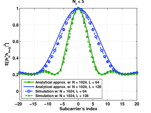
Figure 1: Correlation between subcarriers $E|\bar{\bm{h}}_{n}^{\dagger}\bar{\bm{h}}_{n+q}|^{2}$ from both simulation and analytical results with $N_{t}=5$, $N=1024$, and $L=64\text{ and }128$.

Fig. 2 shows the average received power per subcarrier $\eta_{\text{AVE}}$ with constant interpolation for different numbers of feedback bits $B$ and channel taps $L$. We set the number of transmit antennas $N_{t}=4$, cluster size $M=32$, and SNR at 10 dB. We also place another x-axis on the top of the figure showing the number of bits per cluster $B/K$. In the figure, the solid lines show the analytical approximation given in Corollary 24 while the square and circular markers show the simulation results. Due to search complexity of RVQ, there are no simulation results for a large-feedback regime.

We note from the figure that the average received power increases with $B$ as expected and decreases with $L$. As the channel becomes more frequency selective, the cluster size should be reduced to maintain the performance. We observe that in this example, the analytical results are very close to those from the simulation. Unlike the achievable rate analysis, Jensen’s inequality is not used in deriving $\eta_{\text{AVE}}$. From the figure, we see that about half a feedback bit per subcarrier gives us close to the infinite-feedback performance.

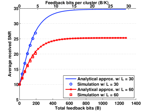
Figure 2: Average received power per subcarrier $\eta_{\text{AVE}}$ with the number of total feedback bits $B$ for $N=1024$, $N_{t}=4$, $M=32$, and SNR at $10$ dB.

Fig. 3 shows the sum achievable rate with constant interpolation with cluster size $M$ from both the analytical approximation from Proposition 1 and the simulation results when the number of total feedback bits is severely limited at 16 bits. Different plots correspond to different $L$ values. For small $M$, more beamforming vectors are quantized and fed back from the receiver, but with a smaller number of feedback bits per cluster. For large $M$, the opposite is true. Thus, there exists an optimal $M$ that maximizes the achievable rate. We can observe from this figure, selecting optimal $M=16$ performs 35% better than that for feeding back every subcarrier ($M=1$) for $L=4$. Comparing the analytical approximation and the simulation results, we observe that the gap is quite substantial (due to Jensen’s inequality); however, the analytical result still can accurately predict the optimal $M$. For a flat fading channel ($L=1$), all subcarrier gains are the same and thus, the optimal $M^{*}=1$. For frequency selective fading ($L>1$), subcarriers are less correlated and the optimal $M^{*}$ decrease with $L$. We remark that the system size for this figure is set to be smaller than that in the previous figure. This is due again to computational complexity of RVQ when $B$ is large.

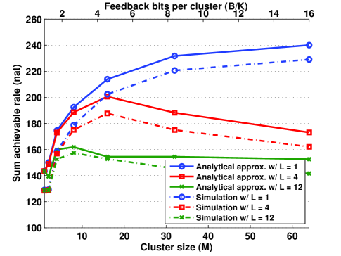
Figure 3: Sum achievable rate with different cluster size $M$ and different number of channel taps $L$ for $N=64$, $N_{t}=4$, $B=16$, and SNR at 10 dB.

Fig. 4 shows the optimal number of subcarriers per cluster $M^{*}$ obtained from the analytical bound approximation with different numbers of channel taps and total feedback bits. In this figure, we observe that $M^{*}$ decreases when $L$ increases. In other words, when the channel becomes more frequency selective, cluster size should be reduced. Furthermore, with more available feedback bits, cluster size should also be reduced. The explanation is as follows. As shown in Fig. 2, an increase in the number of quantization or feedback bits beyond a certain point will give diminishing rate return. Therefore, to extend a rate increase, cluster size should be reduced for a better interpolation of transmit beamforming.

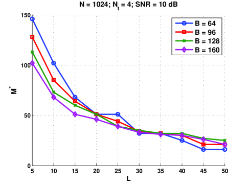
Figure 4: The optimal $M^{*}$ shown with $L$ and $B$ for $N=1024$, $N_{t}=4$, and SNR at 10 dB.

In Fig. 5, we compare the sum achievable rate of all interpolation methods proposed in the study with either the optimized cluster size obtained from (19) or fixed cluster size $M=16$. For this figure, we set $N=256$, $L=24$, $N_{t}=3$, and SNR at 10 dB. We observe that with a low feedback, the performance of interpolation with optimal cluster size and that with $M=16$ do not differ much. However,the performance gap between interpolation with or without the optimized cluster size widens significantly as available feedback becomes larger. The gain on the performance gain could be as high as 15% for the constant interpolation. The solid line on the top of the figure shows the infinite feedback performance. We see that with only two bits per subcarriers, our proposed methods achieve near optimal performance. We note that the second-order interpolation performs worse than the constant or the first-order interpolation in low or moderate $B$ regimes. This is due to the extra feedback bits required to feed back the two phase-rotation parameters $\theta_{m;-1}$ and $\theta_{m;1}$ by the second-order method. The additional feedback bits can be significant. For a fixed $M=16$ (hence, $K=16$), 8 bits per cluster or total 128 bits are used to feed back the two phase-rotation parameters.

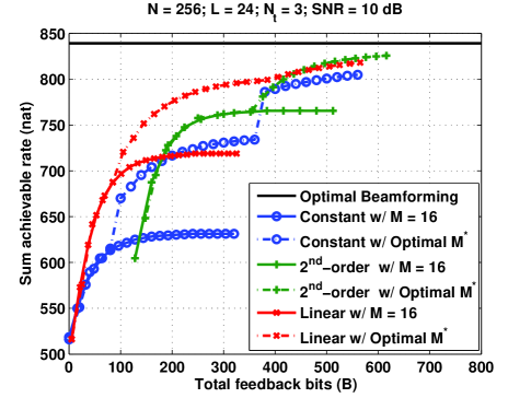
Figure 5: Comparison of the sum achievable rate with different interpolation methods and with either optimized or fixed cluster sizes for $N=256$, $L=24$, $N_{t}=3$, and SNR at $10$ dB.

In Fig. 6, we compare our linear interpolation method with the optimized subcarrier cluster size from Section III and direct channel quantization from Section IV with existing methods [5, 21, 12, 7]. References [5, 21, 12] propose a beamforming interpolation in frequency domain while [7] proposes to vector-quantize channel impulse response. In both [5, 21], a single phase-rotation parameter is used for the whole cluster. Hence, the number of phase rotations to be quantized and fed back in [5, 21] equals the number of clusters. The main difference between [5] and [21] is linear weight $c_{m}$. In our method, the phase rotation $\theta_{m}$ differs for different subcarriers in the same cluster and can be determined at the transmitter with just the number of channel taps $L$ and cluster size $M$ fed back to the transmitter. Thus, the additional number of feedback bits in our method is minimal while those in [5, 21] increase linearly with the number of clusters $K$. For this figure, methods proposed by [5, 21] require 64 additional bits. In [12], phase rotation is based on the chordal distance between the two adjacent quantized beamformers and is the same for all subcarriers in the cluster. References [5, 21, 12] do not optimize cluster size and in this figure, it is fixed at 16. For [7], magnitudes and phases of all channel taps are vector-quantized. The method proposed in [7] performs worse than our channel quantization for small $B$. However, we expect the performance of the two methods to be comparable when $B$ is large.

From Fig. 6, we remark that the combination of our methods (linear interpolation in a low feedback-rate regime and direct channel quantization in a high feedback-rate regime) dominates all mentioned works in all feedback range. Also from this figure, we can conclude that with roughly one feedback bit per subcarrier, the direct channel-tap quantization is preferred, and with fewer than one bit per subcarrier, interpolation from quantized transmit beamformers is preferred.

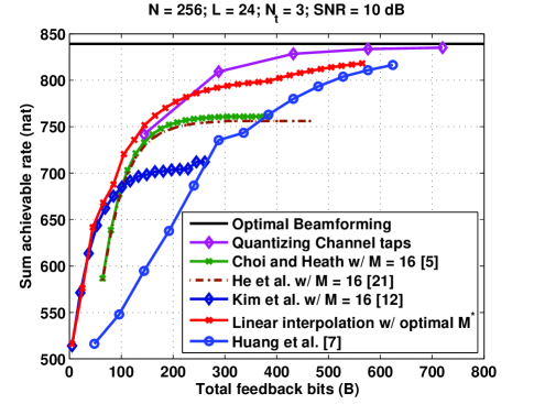
Figure 6: Sum achievable rate of a $3\times 1$ OFDM channel with various feedback schemes plotted with the total number of feedback bits $B$ and $N=256$, $L=24$, and SNR at 10 dB.

In Fig. 7, we compare an achievable rate per subcarrier of a $3\times 1$ channel obtained from simulation and the approximation (55) for a direct quantization of channel taps. A number of channel taps $L$ varies between 32 and 128. From the figure, the approximate sum rate exhibits the same performance trend as the simulation results and the gap between the two is about 10%. Again we can attribute the gap between the two results to Jensen’s inequality. Although the approximation is derived for a large feedback rate, it seems to predict well the simulation result even with relatively small $B$. In addition, we observe from the simulation results that approximately 3 bits per real coefficient are needed to achieve close to the maximum achievable rate. While the number of fading paths $L$ increases, $B$ also increases to achieve close to the maximum rate.

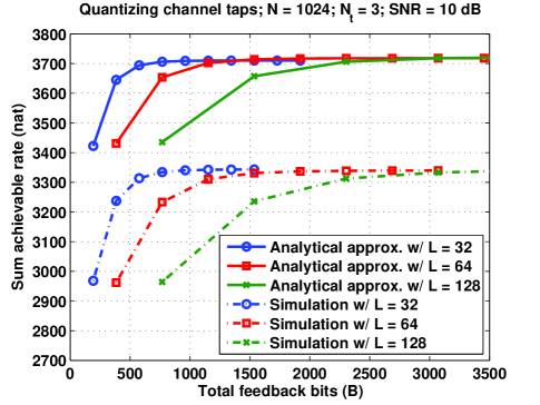
Figure 7: Comparison between achievable rate obtained from simulation and the analytical approximation for channel-tap quantization with $N=1024$, $N_{t}=3$, and SNR at 10 dB.

In Figs. 8 and 9, we compare sum rate of our linear interpolation method with those of perfect transmit beamforming (infinite feedback) and random transmit beamforming (zero feedback). In Fig. 8, we plot sum achievable rates with the number of transmit antennas for $N=256$, $L=24$, and SNR at 10 dB. We see that the sum rates of the perfect beamforming and the linear interpolation with $B=128$ bits increase with $N_{t}$. The gap between the perfect beamforming and our method grows larger as $N_{t}$ increases. To close the gap, more feedback bits are needed for quantizing transmit beamformers.

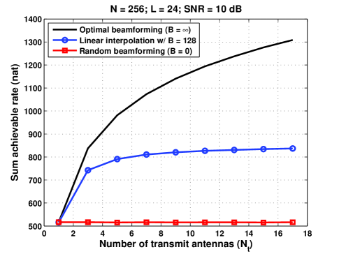
Figure 8: Sum achievable rates of the proposed linear interpolation method, the perfect transmit beamforming, and random beamforming are plotted with $N_{t}$ for $N=256$, $L=24$ and SNR = 10 dB.

In Fig. 9, sum rates are plotted with SNR while $N_{t}=3$. As expected, all sum rates increase with SNR. We also add the performance of channel quantization with $B=288$ or 1.125 bits per subcarrier, which is close to that of the perfect transmit beamforming. The linear interpolation with only 32 bits or 0.125 feedback bits per subcarrier can significantly outperform random beamforming or a system with zero feedback.

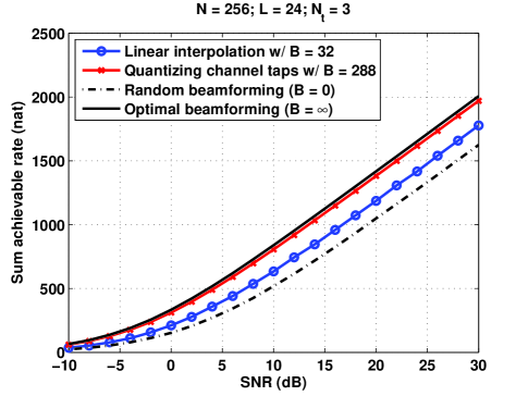
Figure 9: Sum achievable rates from various methods are plotted with SNR for $N=256$, $L=24$ and $N_{t}=3$.

VI Conclusions

We have proposed feedback methods for MISO-OFDM channels. Beamforming interpolation with RVQ performs well with limited feedback while direct quantization of the channel impulse response performs well with large feedback. Thus, switching between the two methods for different feedback rates is recommended. We analyzed the sum achievable rate with constant interpolation and RVQ and showed that the analytical results can predict the performance trend and accurately predict the optimal cluster size. From numerical examples shown, operating at the optimal cluster size can give a significant rate gain over an arbitrary size. For a relatively static channel in which the number of channel taps or SNR do not change often, the cluster size does not have to be updated frequently as well.

For linear interpolation, we have derived a closed-form expression for a phase rotation to avoid exhaustive search and additional number of feedback bits in quantizing the phase rotation. We also considered the higher-order interpolation inspired from the OFDM channel estimation problem. Both linear and higher-order interpolations are improved significantly with the optimized cluster size derived for the constant interpolation. Furthermore, we have analyzed the achievable rate with direct quantization of channel taps, which depends on the feedback rate and the number of antennas and channel taps.

Future work can take different directions. In the problem considered, the MISO channel was investigated. Extending our results to MIMO beamforming is not straightforward and thus, MIMO beamforming could be a good problem to consider. In addition, here we considered channels with a uniform power delay profile. Other practical channel models might be of interest.

-A Proof of Lemma 1

We approximate

$$E\left[|\bar{\bm{h}}_{n}^{{\dagger}}\bar{\bm{h}}_{n+q}|^{2}\right]\approx\frac{E\left[|\bm{h}_{n}^{{\dagger}}\bm{h}_{n+q}|^{2}\right]}{E\left[\|\bm{h}_{n}\|^{2}\|\bm{h}_{n+q}\|^{2}\right]}.$$ (56)

First, we evaluate $E\left[|\bm{h}_{n}^{{\dagger}}\bm{h}_{n+q}|^{2}\right]$ as follows

$$E \left[|\bm{h}_{n}^{{\dagger}}\bm{h}_{n+q}|^{2}\right]=E\left[\left|\sum_{m=1}^{N_{t}}h_{n,m}^{*}h_{n+q,m}\right|^{2}\right]$$ (57)

$$=\sum_{m_{1}=1}^{N_{t}}E\left[|h_{n,m_{1}}|^{2}|h_{n+q,m_{1}}|^{2}\right]$$

$$\quad+\sum_{m_{2}=1}^{N_{t}}\sum_{\begin{subarray}{c}m_{2}=1\\ m_{2}\neq m_{1}\end{subarray}}^{N_{t}}E[h_{n,m_{1}}^{*}h_{n+q,m_{1}}]E[h_{n,m_{2}}h_{n+q,m_{2}}^{*}]$$ (58)

$$=N_{t}E\left[|h_{n,m_{1}}|^{2}|h_{n+q,m_{1}}|^{2}\right]$$

$$\quad+N_{t}(N_{t}-1)|E\left[h_{n,m_{1}}^{*}h_{n+q,m_{1}}\right]|^{2}$$ (59)

where we apply the assumption that channel gains across antennas are i.i.d.

Next we evaluate each term in (59) by substituting (1).

$$E\left[|h_{n}|^{2}|h_{n+q}|^{2}\right]\\ =\sum_{l_{1},l_{2},l_{3},l_{4}=1}^{L}E\left[g_{l_{1}}g_{l_{2}}^{*}g_{l_{3}}g_{l_{4}}^{*}\mathrm{e}^{\frac{-j2\pi\{(l_{1}-l_{2}+l_{3}-l_{4})n+(l_{3}-l_{4})q\}}{N}}\right]$$ (60)

where we omit the antenna subscript $m_{1}$ for brevity. It is straightforward to show that

$$E[g_{l_{1}}g_{l_{2}}^{*}g_{l_{3}}g_{l_{4}}^{*}\mathrm{e}^{\frac{-j2\pi\{(l_{1}-l_{2}+l_{3}-l_{4})n+(l_{3}-l_{4})q\}}{N}}]\\ =\left\{\begin{array}[]{l@{\quad:\quad}l}\frac{2}{L}&l_{1}=l_{2}=l_{3}=l_{4},\\ 1-\frac{1}{L}&(l_{1}=l_{2})\neq(l_{3}=l_{4}),\\ \frac{1}{L}(\varphi^{2}(q)-1)&(l_{1}=l_{3})\neq(l_{2}=l_{4}),\\ 0&\text{otherwise}.\end{array}\right.$$ (61)

Substituting (61) into (60) gives

$$E\left[|h_{n}|^{2}|h_{n+q}|^{2}\right]=1+\frac{1}{L^{2}}\varphi^{2}(q)$$ (62)

Also,

$$E\left[h_{n}^{*}h_{n+q}\right] =\sum_{l_{1}=1}^{L}E|g_{l_{1}}|^{2}\mathrm{e}^{\frac{-j2\pi l_{1}q}{N}}$$

$$\quad+\sum_{l_{1}=1}^{L}\sum_{\begin{subarray}{c}l_{2}=1\\ l_{2}\neq l_{1}\end{subarray}}^{L}E[g_{l_{1}}^{*}g_{l_{2}}]\mathrm{e}^{\frac{-j2\pi l_{1}n}{N}}\mathrm{e}^{\frac{-j2\pi l_{2}(n+q)}{N}}$$ (63)

$$=\sum_{l_{1}=1}^{L}\frac{1}{L}\mathrm{e}^{\frac{-j2\pi l_{1}q}{N}}$$ (64)

$$=\frac{1}{L}\mathrm{e}^{\frac{-j2\pi(L-1)q}{N}}\varphi(q).$$ (65)

where the second term in (63) is equal to zero.

Substituting (62) and (65) into (59) gives

$$E\left[|\bm{h}_{n}^{{\dagger}}\bm{h}_{n+q}|^{2}\right]=N_{t}+\frac{N_{t}}{L^{2}}\varphi^{2}(q).$$ (66)

Following similar steps as the above evaluation of $E\left[|\bm{h}_{n}^{{\dagger}}\bm{h}_{n+q}|^{2}\right]$, we can show that

$$E\left[\|\bm{h}_{n}\|^{2}\|\bm{h}_{n+q}\|^{2}\right]=N_{t}^{2}+\frac{N_{t}}{L^{2}}\varphi^{2}(q).$$ (67)

Substituting (66) and (67) into (56) yields the Lemma.

-B Proof of Proposition 1

From (8),

$$C_{n+q} =E\left[\log(1+\rho\|\bm{h}_{n+q}\|^{2}|\bar{\bm{h}}_{n+q}^{{\dagger}}\hat{\bm{v}}_{n+q}|^{2})\right]$$ (68)

$$\leq\log(1+\rho E[\|\bm{h}_{n+q}\|^{2}|\bar{\bm{h}}_{n+q}^{{\dagger}}\hat{\bm{v}}_{n+q}|^{2}])$$ (69)

$$=\log(1+\rho E\|\bm{h}_{n+q}\|^{2}E|\bar{\bm{h}}_{n+q}^{{\dagger}}\hat{\bm{v}}_{n+q}|^{2})$$ (70)

$$=\log(1+\rho N_{t}E|\bar{\bm{h}}_{n+q}^{{\dagger}}\hat{\bm{v}}_{n+q}|^{2})$$ (71)

where Jensen’s inequality is applied in (69). Eq (70) is due to the fact that $\|\bm{h}_{n+q}\|^{2}$ and $|\bar{\bm{h}}_{n+q}^{{\dagger}}\hat{\bm{v}}_{n+q}|^{2}$ are independent [25]. In addition, $E\|\bm{h}_{n+q}\|^{2}=N_{t}$ since each element in $\bm{h}_{n+q}$ has unit variance. Jensen’s inequality is tighter when the number of transmit antennas increases.

To derive the upper bound on $C_{n+q}$ in (71), we need to determine $E|\bar{\bm{h}}_{n+q}^{{\dagger}}\hat{\bm{v}}_{n+q}|^{2}$. With constant interpolation, $\hat{\bm{v}}_{n+q}$ is set to equal the representative beamforming of a cluster, which is $q$ subcarriers away. Therefore, we would like to evaluate $E|\bar{\bm{h}}_{n+q}^{{\dagger}}\hat{\bm{v}}_{n}|^{2}$. To accomplish this goal, we project $\bar{\bm{h}}_{n+q}$ onto $\bar{\bm{h}}_{n}$ and its $N_{t}-1$-dimensional orthogonal complement denoted by $\bar{\bm{h}}_{n}^{\perp}$.

Let $\{\bm{u}_{1},\bm{u}_{2},\ldots,\bm{u}_{N_{t}-1}\}$ be a basis of $\bar{\bm{h}}_{n}^{\perp}$. Hence, we can write $\bar{\bm{h}}_{n+q}$ as a linear combination of its projection onto $\bar{\bm{h}}_{n}$ and the basis of $\bar{\bm{h}}_{n}^{\perp}$ as follows.

$$\bar{\bm{h}}_{n+q}=(\bar{\bm{h}}_{n}^{{\dagger}}\bar{\bm{h}}_{n+q})\bar{\bm{h}}_{n}+\sum_{i=1}^{N_{t}-1}(\bm{u}_{i}^{\dagger}\bar{\bm{h}}_{n+q})\bm{u}_{i}.$$ (72)

With (72), we have

$$E \left[|\bar{\bm{h}}_{n+q}^{{\dagger}}\hat{\bm{v}}_{n}|^{2}\right]$$

$$=E\left|(\bar{\bm{h}}_{n+q}^{\dagger}\bar{\bm{h}}_{n})(\bar{\bm{h}}_{n}^{{\dagger}}\hat{\bm{v}}_{n})+\sum_{i=1}^{N_{t}-1}(\bar{\bm{h}}_{n+q}^{\dagger}\bm{u}_{i})(\bm{u}_{i}^{{\dagger}}\hat{\bm{v}}_{n})\right|^{2}$$ (73)

$$=E\left[|\bar{\bm{h}}_{n+q}^{\dagger}\bar{\bm{h}}_{n}|^{2}|\bar{\bm{h}}_{n}^{{\dagger}}\hat{\bm{v}}_{n}|^{2}\right]+\sum_{i=1}^{N_{t}-1}E\left[|\bar{\bm{h}}_{n+q}^{{\dagger}}\bm{u}_{i}|^{2}|\bm{u}_{i}^{{\dagger}}\hat{\bm{v}}_{n}|^{2}\right]$$

$$\quad+2E\Re\left\{(\bar{\bm{h}}_{n+q}^{\dagger}\bar{\bm{h}}_{n})(\bar{\bm{h}}_{n}^{{\dagger}}\hat{\bm{v}}_{n})\sum_{i=1}^{N_{t}-1}(\bar{\bm{h}}_{n+q}^{{\dagger}}\bm{u}_{i})(\bm{u}_{i}^{{\dagger}}\hat{\bm{v}}_{n})\right\}$$ (74)

where $\Re\left\{x\right\}$ is the real part of $x$. Similar to [25], it can be shown that $|\bar{\bm{h}}_{n+q}^{{\dagger}}\bar{\bm{h}}_{n}|^{2}$ and $|\bar{\bm{h}}_{n}^{{\dagger}}\hat{\bm{v}}_{n}|^{2}$ are independent. In [25], $E|\bar{\bm{h}}_{n}^{{\dagger}}\hat{\bm{v}}_{n}|^{2}$ was also analyzed while $E|\bar{\bm{h}}_{n+q}^{{\dagger}}\bar{\bm{h}}_{n}|^{2}\approx\psi(q,N_{t})$ from Lemma 1. Thus,

$$E[|\bar{\bm{h}}_{n+q}^{{\dagger}}\bar{\bm{h}}_{n}|^{2} |\bar{\bm{h}}_{n}^{{\dagger}}\hat{\bm{v}}_{n}|^{2}]$$

$$=E|\bar{\bm{h}}_{n+q}^{{\dagger}}\bar{\bm{h}}_{n}|^{2}E|\bar{\bm{h}}_{n}^{{\dagger}}\hat{\bm{v}}_{n}|^{2}$$ (75)

$$\approx\psi(q,N_{t})\left(1-2^{B/K}\beta(2^{B/K},\frac{N_{t}}{N_{t}-1})\right).$$ (76)

For the second term on the right-hand side of (74), we have that similar to the first term,

$$E\left[|\bar{\bm{h}}_{n+q}^{{\dagger}}\bm{u}_{i}|^{2}|\bm{u}_{i}^{{\dagger}}\hat{\bm{v}}_{n}|^{2}\right]=E|\bar{\bm{h}}_{n+q}^{{\dagger}}\bm{u}_{i}|^{2}E|\bm{u}_{i}^{{\dagger}}\hat{\bm{v}}_{n}|^{2}.$$ (77)

We can evaluate the second term in (77) as follows. Similar to (72), we can write $\hat{\bm{v}}_{n}$ as a linear combination of its projection onto basis $\{\bar{\bm{h}}_{n},\bm{u}_{1},\ldots,\bm{u}_{N_{t}-1}\}$ as follows:

$$\hat{\bm{v}}_{n}=(\bar{\bm{h}}_{n}^{\dagger}\hat{\bm{v}}_{n})\bar{\bm{h}}_{n}+\sum_{i=1}^{N_{t}-1}(\bm{u}_{i}^{\dagger}\hat{\bm{v}}_{n})\bm{u}_{i}.$$ (78)

Evaluating $(\hat{\bm{v}}_{n}^{\dagger}\hat{\bm{v}}_{n})^{2}$ with (78) and applying the fact that $\|\hat{\bm{v}}_{n}\|=1$ results in

$$|\bar{\bm{h}}_{n}^{{\dagger}}\hat{\bm{v}}_{n}|^{2}+\sum_{i=1}^{Nt-1}|\bm{u}_{i}^{{\dagger}}\hat{\bm{v}}_{n}|^{2}=1.$$ (79)

We take expectation on both sides and substitute a closed-form expression of $E|\bar{\bm{h}}_{n}^{{\dagger}}\hat{\bm{v}}_{n}|^{2}$ from [25]. Also, $E|\bm{u}_{i}^{\dagger}\hat{\bm{v}}_{n}|^{2}$ is the same for all $1\leq i\leq N_{t}-1$ due to identical distributions. Thus, from (79), we have

$$E|\bm{u}_{i}^{{\dagger}}\hat{\bm{v}}_{n}|^{2}=\frac{2^{B/K}\beta(2^{B/K},\frac{N_{t}}{N_{t}-1})}{N_{t}-1}.$$ (80)

Similar to the steps that derive (80), we can show that

$$E|\bar{\bm{h}}_{n+q}^{{\dagger}}\bm{u}_{i}|^{2}\approx\frac{1-\psi(q,N_{t})}{N_{t}-1}.$$ (81)

Applying (80) and (81), we have

$$\sum_{i=1}^{N_{t}-1}E\left[|\bar{\bm{h}}_{n+q}^{{\dagger}}\bm{u}_{i}|^{2}|\bm{u}_{i}^{{\dagger}}\hat{\bm{v}}_{n}|^{2}\right]\\ \approx(1-\psi(q,N_{t}))\cdot\frac{2^{B/K}\beta(2^{B/K},\frac{N_{t}}{N_{t}-1})}{N_{t}-1}$$ (82)

Evaluating the final term of the right-hand side of (74) is not tractable. However we note that for both small and large feedback, the term is close to zero due to $\bar{\bm{h}}_{n}^{{\dagger}}\hat{\bm{v}}_{n}$ and $\bm{u}_{i}^{{\dagger}}\hat{\bm{v}}_{n}$, respectively. Thus, we approximate

$$E\Re\left\{(\bar{\bm{h}}_{n+q}^{\dagger}\bar{\bm{h}}_{n})(\bar{\bm{h}}_{n}^{{\dagger}}\hat{\bm{v}}_{n})\sum_{i=1}^{N_{t}-1}(\bar{\bm{h}}_{n+q}^{{\dagger}}\bm{u}_{i})(\bm{u}_{i}^{{\dagger}}\hat{\bm{v}}_{n})\right\}\approx 0.$$ (83)

Finally, substituting (76), (82), and (83) in (74) yields Proposition 1.

-C Proof of Proposition 2

Applying the linear interpolation (25) and assuming optimal, unquantized beamforming, we have

$$E|(\bm{v}_{kM}^{\mathrm{opt}})^{\dagger}\bm{v}_{kM+m}|^{2}\\ \approx\frac{E\left|\bm{h}_{kM}^{{\dagger}}\left\{(1-c_{m})\bm{h}_{kM}+c_{m}\mathrm{e}^{j\theta_{m}}\bm{h}_{(k+1)M}\right\}\right|^{2}}{E\|(1-c_{m})\bm{h}_{kM}+c_{m}\mathrm{e}^{j\theta_{m}}\bm{h}_{(k+1)M}\|}.$$ (84)

Here we propose to set phase rotation $\theta_{m}$ by solving

$$\frac{E\left|\bm{h}_{kM}^{{\dagger}}\left\{(1-c_{m})\bm{h}_{kM}+c_{m}\mathrm{e}^{j\theta_{m}}\bm{h}_{(k+1)M}\right\}\right|^{2}}{E\|(1-c_{m})\bm{h}_{kM}+c_{m}\mathrm{e}^{j\theta_{m}}\bm{h}_{(k+1)M}\|}=\psi(m,N_{t}).$$ (85)

where $\psi(m,N_{t})$ is defined in Lemma 1.

Similar to steps shown in the proof of Lemma 1, we can show that

$$E\left|\bm{h}_{kM}^{{\dagger}}\left\{(1-c_{m})\bm{h}_{kM}+c_{m}\mathrm{e}^{j\theta_{m}}\bm{h}_{(k+1)M}\right\}\right|^{2}\\ =(1-c_{m})^{2}(N_{t}+1)+c_{m}^{2}\left(\frac{N_{t}}{L}\varphi(M)^{2}+1\right)\\ +2(1-c_{m})c_{m}\cos\theta_{m}\cos\left(\frac{\pi M(L-1)}{N}\right)\left(\frac{N_{t}+1}{L}\right)\varphi(M)$$ (86)

and

$$E\|(1-c_{m})\bm{h}_{kM}+c_{m}\mathrm{e}^{j\theta_{m}}\bm{h}_{(k+1)M}\|\\ =(1-c_{m})^{2}(N_{t}+1)+c_{m}^{2}N_{t}\\ +2\frac{N_{t}}{L}(1-c_{m})c_{m}\cos\theta_{m}\cos\left(\frac{\pi M(L-1)}{N}\right)\varphi(M).$$ (87)

Substituting (86) and (87) into (84) and solving for $\theta_{m}$ gives Proposition 2.

References

- [1] T. K. Y. Lo, “Maximum ratio transmission,” IEEE Trans. Commun., vol. 47, no. 10, pp. 1458–1461, Oct. 1999.
- [2] W. Santipach and M. L. Honig, “Capacity of a multiple-antenna fading channel with a quantized precoding matrix,” IEEE Trans. Inf. Theory, vol. 55, no. 3, pp. 1218–1234, Mar. 2009.
- [3] D. J. Love, R. W. Heath, Jr., V. K. N. Lau, D. Gesbert, B. D. Rao, and M. Andrews, “An overview of limited feedback in wireless communication systems,” IEEE J. Sel. Areas Commun., vol. 26, no. 8, pp. 1341–1365, Oct. 2008.
- [4] M. Wu, C. Zhen, and Z. Qui, “Feedback reduction based on clustering in MIMO-OFDM beamforming systems,” in Proc. IEEE Int. Conf. on Wireless Commun., Networking and Mobile Computing (WiCom), Beijing, China, Sep. 2009, pp. 1–4.
- [5] J. Choi and R. W. Heath, Jr., “Interpolation based transmit beamforming for MIMO-OFDM with limited feedback,” IEEE Trans. Signal Process., vol. 53, no. 11, pp. 4125 – 4135, Nov. 2005.
- [6] C. He, P. Zhu, B. Sheng, and X. You, “Two novel interpolation algorithms for MIMO-OFDM systems with limited feedback,” in Proc. IEEE Veh. Technol. Conf. (VTC Fall), San Francisco, CA, USA, Sep. 2011. ISSN 1090-3038 pp. 1–5.
- [7] Q. Huang, M. Ghogho, Y. Li, D. Ma, and J. Wei, “Transmit beamforming for MISO frequency-selective channels with per-antenna power constraint and limited-rate feedback,” IEEE Trans. Veh. Technol., vol. 60, no. 8, pp. 3726–3735, Oct. 2011.
- [8] H. Z. Ye, V. Stolpaman, and N. van Waes, “A reduced CSI feedback approach for precoded MIMO-OFDM system,” IEEE Trans. Wireless Commun., vol. 6, no. 1, pp. 55–58, Jan. 2007.
- [9] H. Long, K. J. Kim, W. Xiang, S. Shen, K. Zheng, and W. Wang, “Improved wideband precoding with arbitrary subcarrier grouping in MIMO-OFDM systems,” IET Commun., vol. 6, no. 3, pp. 281–288, Feb. 2012.
- [10] T. Pande, D. J. Love, and J. V. Krogmeier, “Reduced feedback MIMO-OFDM precoding and antenna selection,” IEEE Trans. Signal Process., vol. 55, no. 5, pp. 2284–2293, May 2007.
- [11] J. Huang, J. Zhang, Z. Liu, J. Li, and X. Li, “Transmit beamforming for MIMO-OFDM systems with limited feedback,” in Proc. IEEE Veh. Technol. Conf. (VTC Fall), Calgary, BC, Sep. 2008, pp. 1 – 5.
- [12] J. Kim, B. Kim, J. Lee, and D. Park, “Closed-form interpolations for MISO-OFDM beamforming codewords,” in Proc. Int. Conf. on Inf. and Commun. Technol. Convergence (ICTC), Jeju, Korea, Nov. 2010, pp. 43–44.
- [13] H. He and Y. Zeng, “Transmit beamforming interpolation algorithm for MIMO-OFDM systems in the limited feedback scenario,” in Proc. IEEE Int. Conf. on Computer and Inf. Technol. (CIT), Chengdu, Sichuan, China, Oct. 2012, pp. 696 – 699.
- [14] J. Chang, I. T. Lu, and Y. X. Li, “Adaptive codebook-based channel prediction and interpolation for multiuser multiple-input multiple-output orthogonal frequency division multiplexing systems,” ETRI Journal, vol. 34, no. 1, pp. 9–16, Feb. 2012.
- [15] L. Wang and C. H. B. Sheng, “Study on feedback reduction techniques in MIMO-OFDM beamforming systems,” in Proc. Int. Conf. on Wireless Commun. and Signal Process. (WCSP), Huangshan, Anhui, China, Oct. 2012, pp. 1–5.
- [16] S. Zhou, B. Li, and P. Willett, “Recursive and trellis-based feedback reduction for MIMO-OFDM with rate-limited feedback,” IEEE Trans. Wireless Commun., vol. 5, no. 12, pp. 3400–3405, Dec. 2006.
- [17] B. Zhao, T. Akbudak, M. Simsek, A. Czylwik, and H. Xu, “Limited feedback for MISO-OFDM systems,” in Proc. Int. OFDM Workshop (InOWo), Duisburg, Germany, Aug. 2012, pp. 1–4.
- [18] T. Ghirmai, “Design of reduced complexity feedback precoding for MIMO-OFDM,” Int. J. Commun. Syst., 2014. doi: 10.1002/dac.2806
- [19] G. S. Liu and C. H. Wei, “A new variable fractional sample delay filter with nonlinear interpolation,” IEEE Trans. Circuits Syst. II, vol. 93, no. 2, pp. 1057–7130, Feb. 1992.
- [20] M. H. Hsieh and C. H. We, “Channel estimation for OFDM systems based on comb-type pilot arrangement in frequency selective fading channels,” IEEE Trans. Consum. Electron., vol. 44, no. 1, pp. 217 – 225, Feb. 1998.
- [21] C. He, Z. Peng, Q. Zeng, and Y. Zeng, “A novel OFDM interpolation algorithm based on comb-type pilot,” in Proc. IEEE Int. Conf. on Wireless Commun., Networking and Mobile Computing (WiCom), Beijing, China, Sep. 2009, pp. 893–896.
- [22] M. Diallo, M. Hélard, and L. Cariou, “A limited and efficient quantized feedback for IEEE 802.11n evolution,” in Proc. IEEE Int. Conf. on Telecommun. (ICT), Casablanca, Morocco, May 2013, pp. 1–5.
- [23] K. Mamat and W. Santipach, “Subcarrier clustering for MISO-OFDM channels with quantized beamforming,” in Proc. Int. Conf. on Electrical Engineering/Electronics, Computer, Telecommun. and Inf. Technol. (ECTI-CON), Huahin, Thailand, May 2012, pp. 1–4.
- [24] ——, “On transmit beamforming for multiantenna OFDM channels with finite-rate feedback,” in Proc. IEEE Int. Conf. on Commun. (ICC), Budapest, Hungary, Jun. 2013, pp. 5689–5693.
- [25] C. K. Au-Yeung and D. J. Love, “On the performance of random vector quantization limited feedback beamforming in a MISO system,” IEEE Trans. Wireless Commun., vol. 6, no. 2, pp. 458–462, Feb. 2007.
- [26] D. K. Borah and B. D. Hart, “Frequency-selective fading channel estimation with a polynomial time-varying channel model,” IEEE Trans. Commun., vol. 47, no. 6, pp. 862–873, Jun. 1999.
- [27] V. Nguyen, H.-P. Kuchenbecker, H. Haas, K. Kyamakya, and G. Gelle, “Channel impulse response length and noise variance estimation for OFDM systems with adaptive guard interval,” EURASIP J. on Wireless Commun. and Networking, 2007. doi: 10.1155/2007/24342
- [28] D. J. Love, R. W. Heath, Jr., W. Santipach, and M. L. Honig, “What is the value of limited feedback for MIMO channels?” IEEE Commun. Mag., vol. 42, no. 10, pp. 54–59, Oct. 2004.
- [29] N. S. Jayant and P. Noll, Digital Coding of Waveforms: Principles and Applications to Speech and Video. Englewood Cliffs, NJ, USA: Prentice-Hall, 1984.
- [30] Q. Zhang, S. Jin, K.-K. Wong, H. Zhu, and M. Matthaiou, “Power scaling of uplink massive MIMO systems with arbitrary-rank channel means,” IEEE J. Sel. Topics Signal Process., vol. 8, no. 55, pp. 966–981, Oct. 2014.
- [31] D. Hui and D. L. Neuhoff, “Asymptotic analysis of optimal fixed-rate uniform scalar quantization,” IEEE Trans. Inf. Theory, vol. 47, no. 3, pp. 957–977, Mar. 2001.
- [32] J. Bucklew and N. Gallagher, Jr., “A note on optimal quantization,” IEEE Trans. Inf. Theory, vol. 25, no. 3, pp. 365–366, May 1979.