Approach and separation of quantum vortices with balanced cores

Abstract

The scaling laws of isolated quantum vortex reconnection are characterised by numerically integrating the three-dimensional Gross-Pitaevskii equations, the simplest mean-field equation for a quantum fluid. The primary result is the identification of distinctly different temporal power laws for the pre- and post-reconnection separation distances $\delta(t)$ for two configurations. For the initially anti-parallel case, the scaling laws before and after the reconnection time $t_{r}$ obey the dimensional $\delta\sim|t_{r}-t|^{1/2}$ prediction with temporal symmetry about $t_{r}$ and physical space symmetry about the mid-point between the vortices $x_{r}$. The extensions of the vortex lines close to reconnection form the edges of an equilateral pyramid. For all of the initially orthogonal cases, $\delta\sim|t_{r}-t|^{1/3}$ before reconnection and $\delta\sim|t-t_{r}|^{2/3}$ after reconnection, which are respectively slower and faster than the dimensional prediction. For both configurations, smooth scaling laws are generated due to two innovations. One is to initialise with density profiles about the vortex cores that suppress unwanted secondary temporal density fluctuations. The other innovation is the accurate identification of the position of the vortex cores from a pseudo-vorticity constructed on the three-dimensional grid from the gradients of the wave function. These trajectories allow us to calculate the Frenet-Serret frames and the curvature of the vortex lines, secondary results that might hold clues for the origin of the differences between the scaling laws of the two configurations. For the orthogonal cases, the reconnection takes place in a reconnection plane defined by the directions of the curvature and vorticity. To characterise the structure further, lines are drawn that connect the four arms that extend from the reconnection plane, from which four angles $\theta_{i}$ between the lines are defined. Their sum is convex or hyperbolic, that is $\sum_{i=1,4}\theta_{i}>360^{\circ}$, as opposed to the acute angles of the pyramid found for the anti-parallel initial conditions.

1 Background

The term “quantum turbulence” refers to a tangle of quantum vortex lines, a tangle whose formation and decay is determined by how these vortices collide, reconnect and separate. Although superfluid tangles form in a variety of ³He or ⁴He experiments such as counter-flow, moving grids, colliding vortex rings (Skrbek & Sreenivasan, 2012; Walmsley & Golov, 2008), until recently very little has been known directly about the underlying microscopic interactions. Instead, the nature of the vortex interactions has been inferred from how rapidly the tangle decays.

Theoretically, the observed decay has been linked to the conversion of the kinetic energy of the vortices into other forms of energy. This could be conversion into the kinetic energy of the normal component in higher temperature experiments or into the interaction energy and quantum waves in low temperature quantum fluids, including Bose-Einstein condensates. Despite this, most of our current theoretical insight into quantum vortex reconnection has been through Lagrangian, Biot-Savart simulations of isolated vortex filaments, a dynamical system that does not include the terms for the interaction energy. Why?

Part of the reason is that the Lagrangian approach has experimental support, most recently by comparisons between experiments tracking quantum vortices with solid hydrogen particles (Bewley et al., 2008; Paoletti et al., 2008) and the scaling in the filament calculation of initially anti-parallel vortices by de Waele & Aarts (1994). In both cases, the minimum separation distance between vortices, $\delta$, was interpreted in terms of the dimensional analysis based upon the circulation $\Gamma$ of the vortices. That is, if ${\displaystyle\frac{d}{dt}}\delta\sim v\sim\Gamma/\delta$, then one would expect that

$$\delta(t)\sim(\Gamma|t_{r}-t|)^{1/2}\,.$$ (1.1)

This will be called the dimensional scaling.

Alternatively, one can simulate the underlying mean-field equations of quantum fluids and visualise vortex reconnection by following the low density isosurfaces that surround the zero density cores. The problem with this approach is that tracking the motion of the vortices within these isosurfaces is difficult, even for single interactions.

The aim of this paper is to begin to fill that gap using two innovations for solutions of the mean-field, hard-sphere Gross-Pitaevskii equations. One innovation is an initial condition that suppresses fluctuations in the temporal scaling of separations and the second is a method for identifying the position of the vortex cores. These innovations will be used to determine scaling laws for two classes of initial configurations, orthogonal or anti-parallel vortices.

The conclusion will be that the scaling laws for the minimum separation distance between the two vortices in the two configurations are distinctly different, even when the pairs are just several core radii apart. The anti-parallel case obeys the expectations from (1.1), but the orthogonal cases consistently obey a distinctly different type of scaling. The two sets of scaling laws will be associated with differences in the alignment of their respective Frenet-Serret coordinate frames, differences that form almost immediately

This paper is organised as follows. First, the equations and the initialisation of the model are introduced, followed by overviews of the anti-parallel and orthogonal global evolution in three-dimensions. Next, the methods used to identify the trajectories of the vortices and the local properties of the Frenet-Serret frame, including curvature, are explained. The numerical results, arranged by the type of simulation, orthogonal and anti-parallel, are then described. The results include the time dependence of the separation of the vortices, the curvature along the vortices and the alignments in terms of the Frenet-Serret frames. Finally, the differences between the two classes of initial conditions are discussed and how these differences might affect the observed scaling laws for the approach and release of reconnecting vortices.

2 Equations, numerics and initial condition

Following Berloff (2004), the three-dimensional Gross-Piteavskii equations for the complex wave function or order-parameter $\psi$ are

$$\frac{1}{i}\frac{\partial}{\partial t}{\psi}=E_{v}\nabla^{2}\psi+V(|\mbox{\boldmath$x$}-\mbox{\boldmath$x$}^{\prime}|)\psi(1-|\psi|^{2})\quad{\rm with}\quad E_{v}=0.5~{}~{}{\rm and}~{}~{}V(|\mbox{\boldmath$x$}-\mbox{\boldmath$x$}^{\prime}|)=0.5\delta(\mbox{\boldmath$x$}-\mbox{\boldmath$x$}^{\prime})\,.$$ (2.1)

These are the mean-field equations of a microscopic, quantum system with $\hbar$ and $m$ non-dimensionalized to be 1, a chemical potential of $E_{v}=0.5$ and using the hard-sphere approximation for $V(|\mbox{\boldmath$x$}-\mbox{\boldmath$x$}^{\prime}|)$. They are an example of a defocusing nonlinear Schrödinger equation. All calculations in this paper will use (2.1).

These equations conserve mass:

$$M=\int dV|\psi|^{2}$$ (2.2)

and a Hamiltonian

$$H=\frac{1}{2}\int dV\left[\nabla\psi\cdot\nabla\psi^{\dagger}+0.25(1-|\psi|^{2})^{2}\right]$$ (2.3)

where $\psi^{\dagger}$ is the complex conjugate of $\psi$. The local strength of the mass density, kinetic or gradient energy $K_{\psi}$ and the interaction energy $I$ are

$$\rho=|\psi|^{2},\quad K_{\psi}=\frac{1}{2}|\nabla\psi|^{2}\quad{\rm and}\quad I(\mbox{\boldmath$x$})=\frac{1}{4}(1-|\psi|^{2})^{2}$$ (2.4)

Isosurfaces of $\rho$ are used in all the three-dimensional visualisations and $K_{\psi}$ are included in figures 2.1, 2.3, 2.3, 4.4 and 5.1.

Gross-Pitaevskii calculations have previously identified the following features of quantum vortex reconnection. First, it has been demonstrated (Leadbeater et al., 2003; Berloff, 2004; Kerr, 2011) that the line length grows just prior to reconnection, indicating a type of vortex stretching. Second, reconnection radiates energy, either as sound waves (Berloff, 2004; Leadbeater et al., 2001, 2003), non-linear refraction waves (Berloff, 2004; Zuccher et al., 2012) or strongly non-linear vortex rings (Leadbeater et al., 2003; Berloff, 2004; Kerr, 2011). About 10% of the initial kinetic energy $K_{\psi}$ is lost by these means during the initial reconnection (Kerr, 2011). With added terms representing assumptions about the type of energy depletion at small-scales, these equations can also give us hints to why the vortex tangle decays (Sasa et al., 2011).

2.1 Quasi-classical approximations

But how can the continuum Gross-Pitaevskii equations provide us with details about the Lagrangian dynamics and reconnections that underlie the vortex tangle of quantum fluids?

This can be done by writing the wave function as $\psi=\sqrt{\rho}e^{i\phi}$, where $\rho$ is the density and $\phi$ is the complex phase, then defining the phase velocity $\mbox{\boldmath$v$}_{\phi}$ and quantised circulation $\Gamma$ around the line defects:

$$\mbox{\boldmath$v$}_{\phi}=\nabla\phi={\rm Im}(\psi^{\dagger}\nabla\psi)/\rho\qquad\Gamma=\int\mbox{\boldmath$v$}_{\phi}\cdot\mbox{\boldmath$s$}=2\pi$$ (2.5)

then identifing the $\rho\equiv 0$ line defects as quantum vortices whose dimensionless quantised circulation is $\Gamma$. Even though these lines cannot represent a true vorticity field because the vorticity $\mbox{\boldmath$\omega$}=\nabla\times\mbox{\boldmath$v$}_{\phi}=\nabla\times\nabla\cdot\phi\equiv 0$. In this picture, vortex reconnection appears naturally as the instantaneous re-alignment of these lines and exchange of circulation when the line defects meet. If dimensions were added, the quantised circulation has the classical units of circulation: $\Gamma\sim\rho L^{2}/T$. Note these two differences with classical vortices governed by the Navier-Stokes equation: classical circulation is not quantised and viscous reconnection is never 100%.

To extract the Lagrangian motion of quantum vortices from fields defined on three-dimensional meshes these issues must be addressed:

• As the state relaxes from its initial form, it should not be dominated by either interal waves (phonons) or strong fluctuations along the vortex trajectories (Kelvin waves).

• Second, a method is needed for identifying the direction and positions that the vortices follow as they pass through the three-dimensional mesh.

Two innovations introduced in this paper, (2.7) for the initial density and (3.1) for tracking vortices, resolve both problems and allow us to extract smooth motion for the vortices from the calculated solutions of the Gross-Pitaevskii equations on Eulerian meshes.

To complete the discussion of the Gross-Pitaevskii equations (2.1), the full analogy to classical hydrodynamic equations comes from inserting $\psi=\sqrt{\rho}\exp(i\phi)$ into (2.1) to get the standard equation for $\rho$ and a Bernoulli equation for $\phi$:

$${\displaystyle\frac{\partial}{\partial t}}\rho+\nabla\cdot(\rho\mbox{\boldmath$v$}_{\phi})=0\qquad\frac{\partial}{\partial t}\phi+(\nabla\phi)^{2}=0.5(1-\rho)+\nabla^{2}\sqrt{\rho}/\sqrt{\rho}\,.$$ (2.6)

The $\mbox{\boldmath$v$}_{\phi}$ velocity equation can then be formed by taking the gradient of the $\phi$ equation.

As in Kerr (2011), the numerics are a standard semi-implicit spectral algorithm where the nonlinear terms are calculated in physical space, then transformed to Fourier space to calculate the linear terms. In Fourier space, the linear part of the complex equation is solved through integrating factors with the Fourier transformed nonlinearity added as a 3rd-order Runge-Kutta explicit forcing. The domain is imposed by using no-stress cosine transforms in all three directions. For all of the calculations the domain size is $L_{x}\times L_{y}\times L_{z}=(16\pi)^{3}\approx 50^{3}$ or $(32\pi)^{3}$. Both $128^{3}$ and $256^{3}$ grids were used, with the $256^{3}$ grid giving smoother temporal evolution. Most of the analysis and graphics will use the $\delta_{0}=3$, $256^{3}$ calculation.

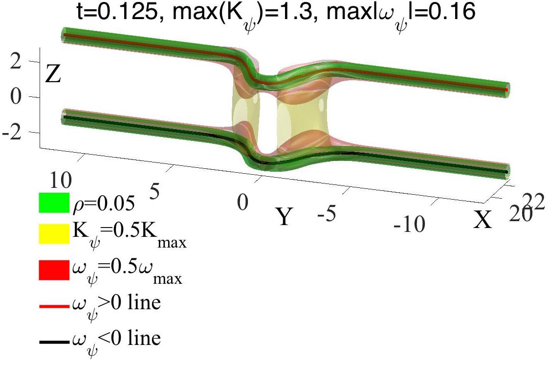
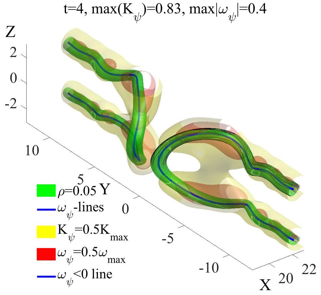
Figure 2.1: Anti-parallel case: Density, kinetic energy $K_{\psi}=|\nabla\psi|^{2}$ and pseudo-vorticity $|\nabla\psi_{r}\times\nabla\psi_{i}|$ isosurfaces plus vortex lines at these times: (a) $t=0.125$, with $\max(K_{\psi})=1.3$, and (b) $t=4$ with $\max(K_{\psi})=0.83$. $\max|\omega_{\psi}|=0.4$ for all the times. The vortex lines show that the pseudo-vorticity method not only follows the lines $\rho=0$ well, but the $t=4$ frame also shows that it can be used to follow isosurfaces of fixed $\rho$. The $t=0.125$ frame shows that initially the kinetic energy is largest between the elbows of the two vortices, with large $\omega_{\psi}$ at the elbows. The $t=4$ frame shows the newly reconnected vortices as they are separating with undulations on the vortex lines that will form additional reconnections and vortex rings at later times.

Figure 2.2: Overview of the evolution of the $\delta_{0}=3$ $256^{3}$ orthogonal calculation from a three-dimensional perspective for two times: $t=6$ as reconnection is beginning and $t=14$ after it has ended, where $t_{r}\approx 8.9$. Green $\rho=0.05$ isosurfaces encase the vortex cores, blue and red lines. The Frenet-Serret frames for $t=8.75$ are given in figure 4.4. A twist in the post-reconnection $t=14$ right ($x>0$) vortex is visible.

Figure 2.3: The same $\delta_{0}=3$ fields and times as in figure 2.3 from the Nazarenko perspective, which looks down the 45^∘ propagation plane in the $y-z$-plane in figure 4.6. This perspective is useful because the pre- and post-reconnection symmetries can be seen most clearly, which is why it is the basis for comparison of reconnection angles in figure 4.6 and section 4.6. The arms are extending away from the reconnection plane, either towards or away from the viewer, Also note that from this perspective, loops are clearly not forming.

2.2 Choice of initial configurations and profiles

Configurations. Two initial vortex configurations are used in this paper, anti-parallel vortices with a perturbation, and orthogonal vortices. Both configurations have been used many times for both classical (Navier-Stokes) and quantum fluids, including the first calculations using the three-dimensional Gross-Pitaevskii equations (Koplik & Levine, 1993).

The advantage of focusing on these configurations is that the interactions leading to reconnection for most other configurations, for example colliding or initially linked, vortex rings, can be reduced to either anti-parallel or orthogonal dynamics, both of which can resolve the reconnection events in smaller global domains. This is because the initial reconnection events require, effectively, only half of each ring.

These two configurations also represent the two extremes for the initial chirality or linking number of the vortex lines in a quantum fluid. In classical fluids the corresponding global property is the helicity, $h=\int(\nabla\times\mbox{\boldmath$u$})\cdot\mbox{\boldmath$u$}\,dV$. When $h$ is large, it tends to suppress nonlinear interactions. Anti-parallel initial conditions have zero net helicity and are sensitive to initial instabilities while orthogonal initial conditions have a large helicity, so reconnection can be delayed (Boratav et al., 1992).

Density profile. The density profiles for all the vortex cores in this paper are determined by the following Padé approximate:

$$\begin{array}[]{c}\vskip 6.0pt plus 2.0pt minus 2.0pt|\psi_{sb}|=\sqrt{\rho_{sb}}=\dfrac{c_{1}r^{2}+c_{2}r^{4}}{1+d_{1}r^{2}+d_{2}r^{4}}\\ {\rm with}\quad c_{1}=0.3437,~{}~{}c_{2}=0.0286,~{}~{}d_{1}=0.3333,~{}~{}{\rm and}~{}~{}d_{2}=0.02864\,.\end{array}$$ (2.7)

Note that $c_{2}\lesssim d_{2}$, which implies that as $r\rightarrow\infty$, the density approaches the usual background of $\rho=1$ from below more slowly than the true Padé of this order does. The true Padé, derived by Berloff (2004), has $c_{2}=d_{2}=11/384\approx 0.02864$. Therefore, the profile with $c_{2}\lesssim d_{2}$ is designated as $\psi_{sb}$ because it is a sub-Berloff (2004) profile. Furthermore, because the calculations are in finite domains, to ensure that the Neumann boundary conditions are met, a set of up to 24 mirror images of the vortices are multiplied together. This multiplication process takes the slight, original $\rho_{sb}<1$ values as $r\rightarrow\infty$ and generates stronger differences. At the boundaries, this gives $(1-\rho)\approx 0.02-0.03$.

For all of the configurations discussed here, using this $|\psi|\lesssim 1$ initial profile appears to be crucial in allowing us to obtain clear scaling laws for the pre- and post-reconnection separation of the vortices. As discussed in subsection 4.2, further tests have confirmed that the temporal separations of all of the true Padé approximates have significant fluctuations.

type	mesh	$\delta_{0}$	$t_{r}$	$K_{\psi}(t=0)$	$I_{0}$
$\perp$ $(16\pi)^{3}$	$256^{3}$	2	2.7	0.0074	0.0023
$\perp$ $(16\pi)^{3}$	$128^{3}$	3	8.9	0.0074	0.0023
$\perp$ $(16\pi)^{3}$	$256^{3}$	3	8.9	0.0074	0.0023
$\perp$ $(16\pi)^{3}$	$256^{3}$	4	21	0.0074	0.0023
$\perp$ $(32\pi)^{2}\times 16\pi$	$256^{2}\times 128$	4	21	0.00178	0.00049
$\perp$ $(32\pi)^{3}$	$256^{3}$	5	40	0.0074	0.0023
$\perp$ $(32\pi)^{3}$	$256^{3}$	6	68	0.0074	0.0023
$\|$ $(16\pi)^{3}$	$256^{3}$	4	2.44	0.0056	0.0031

Table 1: Cases: Type is orthogonal $\perp$ or anti-parallel $\|$, initial separations, approximate reconnection times, initial kinetic and interaction energies.

Once the best profile has been chosen, then one must choose the trajectories of the interacting vortices. The anti-parallel global states are shown first in figure 2.1 as they illustrate the use of all of the three-dimensional diagostics.

2.3 Anti-parallel: Initial trajectory and global development.

Based upon past experience with classical vortices and Kerr (2011), the positions $\mbox{\boldmath$s$}_{\pm}(y)$ of the two nearly anti-parallel $y$-vortices, with a perturbation in the direction of propagation $x$, were

$$\mbox{\boldmath$s$}_{\pm}(y)=\left(\delta_{x}\frac{2}{\cosh\bigl{(}(y/\delta_{y})^{1.8}\bigr{)}}-x_{c},y,\pm z_{c}\right)\,.$$ (2.8)

The parameters used were $\delta_{x}=-1.6$, $\delta_{y}=1.25$, $x_{c}=21.04$ and $z_{c}=2.35$. The power of 1.8 on the normalized position was chosen to help localise the perturbation near the $y=0$ symmetry plane. The density profiles were applied perpendicular to this trajectory, and not perpendicular to the $y$-axis.

As in Kerr (2011), two of the Neumann boundaries act as symmetry planes to increase the effective domain size. These planes are the $y=0$, $x-z$ perturbation plane and $z=0$, $x-y$ dividing plane. Because the goal of this calculation was to focus upon the scaling around the first reconnection, the long domain used in Kerr (2011) to generate a chain of vortices is unnecessary and $L_{y}$ is less. In addition, based upon recent experience with Navier-Stokes reconnection (Kerr, 2013), $L_{z}$ was increased to ensure that the evolving vortices do not see their mirror images across the upper $z$ Neumann boundary condition.

Figure 2.1 shows the state at $t=0.125$, essentially the initial condition, and the state at $t=4$, after the first reconnection event at $t_{r}\approx 2.4$. Three isosurfaces are given. Low density isosurfaces ($\rho=0.05$), isosurfaces of the kinetic energy $K_{\psi}$ (2.4) and isosurfaces of $|\mbox{\boldmath$\omega$}_{\psi}|$ (3.1), a pseudo-vorticity that is introduced in the next section. The vortex lines defined by $\mbox{\boldmath$\omega$}_{\psi}$ and Proposition 1 are shown using thickened curves. The structure at the time of reconnection is discussed in section 5 using Figure 5.1 and how the flow would develop later has already been documented by Kerr (2011), which shows several reconnections forming a stack of vortex rings.

Both $K_{\psi}$ and $\mbox{\boldmath$\omega$}_{\psi}$ are functions of the first-derivatives of the wave function, but show different aspects of the flow. The $K_{\psi}$ isosurfaces show where the momentum is large. Initially, the momentum is dominated by forward motion between the perturbations, as shown for $t=0.125$. Post-reconnection, at $t=4$, the $K_{\psi}$ surfaces show that the primary motion is around the vortices. $|\mbox{\boldmath$\omega$}_{\psi}|$ is large where the vortex cores bulge and have the greatest curvature.

2.4 Orthogonal: Initial separations and global development.

To place the orthogonal vortices one only needs to choose one line parallel to the $y$ axis and another line parallel to the $z$ axis through two points in $x$ on either side of $x=y=z=0$. The five separations and other details of the simulations are given in Table 1. Because all of the orthogonal cases with $\delta_{0}\geq 2$ behave qualitatively in the same manner, all of the orthogonal three-dimensional images will be taken from the $256^{3}$ $\delta_{0}=3$ calculation, whose estimated reconnection is at time $t_{r}=8.9$.

The first two sets of three-dimensional isosurfaces and vortex lines in figures 2.3 and 2.3 are used to show the global evolution of the vortices through reconnection, with figure 2.3 providing a true three-dimensional perspective of the orthogonality and figure 2.3, defined by figure 4.6, providing a perspective down the $y=z$ axis, which is also used for the determination of three-dimensional angles in subsection 4.4. The two times chosen for each are $t=6$, pre-reconnection, and $t=19$, post-reconnection.

The two isosurfaces are for a low density of $\rho=0.05$ and kinetic energy of $K_{\psi}=0.5$, where $\max(K_{\psi})=0.58$. There are two pseudo-vortex lines (3.1) in each frame, one that originates on the $y=0$ plane and the other on the $z=0$ plane. The $t=8.5$ frame also shows some additional orientation vectors that will be discussed in section 4.

Qualitative features are:

• The initially orthogonal vortices are attracted towards each other at their points of closest approach, asymmetrically bending out towards each other.

• During this stage there is a some loss of the kinetic energy between $t=8$ and $t=11$, $\Delta_{t}K_{\psi}<10\%K_{\psi}(t=0)$. This is converted into interaction energy $I$ (2.4). There are no further noticeable changes in $K_{\psi}$ for $t>12$.

• After reconnection, from one perspective there is a slight twist on one vortex, but it is not twisted enough for the vortices to loop back upon themselves and reconnect again. Instead, the two new vortices pull back from one another, as shown by the $t=19$ frame in figure 2.3. Consistent with experimental observations of vortex interactions using solid hydrogen particles (Bewley et al., 2008; Schwarzschild, 2010) in the sense that post-reconnection filaments simply pull back from one another and do not loop.

• Two sketches of the alignments and an addition isosurface perspective are used in subsection 4.3 to illustrate this evolution further.

3 Approach and separation of vortex lines: Methodology

The primary result in this paper will be the differences in the temporal scaling of the pre- and post-reconnection separation of the vortices for the two configurations. The secondary results are clues for the origin of these differences in the evolution of the local curvature and Frenet-Serret frames on the vortices for the two configurations. To achieve this, one needs an initial condition for which the evolution of the vortices is smooth and a means to follow that evolution. The key ingredient of the initial condition is provided by the choice of coefficients in (2.7). This section will show what is needed to accurately track the vortices. Two methods for detecting the vortices have been used.

3.1 Detecting lines by finding $\rho=0$ mesh cells.

The first approach is to estimate the locations of the $\rho\equiv 0$ quantum vortex lines by extracting the positions of the vertices of a $\rho\gtrsim 0$ isosurface mesh, determined by Matlab, then average these positions. For this method to work, the density $\rho$ has to be small enough so that there are only 3-6 points clustered in a plane perpendicular to the vortex lines. The method begins to fail around reconnection points because there is an extensive $\rho\approx 0$ zone as the cores of the vortices start to overlap, resulting in the isosurface points that are too far apart to make reliable estimates for the positions of the $\rho\equiv 0$ cores. Due to these problems, this approach is used only for providing the seeds for our preferred approach and its validation.

3.2 $\mbox{\boldmath$\omega$}_{\psi}=\nabla\rho\times\nabla\phi$ pseudo-vorticity method

The second approach begins by recognising that the line of zero density should be perpendicular to the gradients of the real and imaginary parts of the wave function. Therefore it is useful to define the following pseudo-vorticity:

$$\mbox{\boldmath$\omega$}_{\psi}=0.5\nabla\psi_{r}\times\nabla\psi_{i}$$ (3.1)

The inspiration for this approach comes from how to write the vorticity in terms of a cross production of the scalars in Clebsch pairs, which is an alternative approach to representing the incompressible Euler equations.

Proposition 1

At points with $\rho=0$, the direction of the quantum vortex line is defined by the direction of $\mbox{\boldmath$\omega$}_{\psi}=0.5\nabla\psi_{r}\times\nabla\psi_{i}$.

Proof 3.1.

A quantum vortex line is defined by $\rho\equiv 0$, which because $\rho=\psi_{r}^{2}+\psi_{i}^{2}$ implies that $\psi_{r}=\psi_{i}=0$ on this vortex line.

Then define $\hat{\omega}_{\rho}$ the direction vector of the line at any arbitary point on the vortex line. By the definition of the line, the values of $\psi_{r}$ and $\psi_{i}$ in this direction must not change and thus we know that $\nabla\psi$ must satisfy

$$\hat{\omega}_{\rho}\cdot\nabla\psi_{r}=\hat{\omega}_{\rho}\cdot\nabla\psi_{i}=0$$

at these points. This is only possible if $\hat{\mbox{\boldmath$\omega$}}_{\rho}=(\nabla\psi_{r}\times\nabla\psi_{i})/|\nabla\psi_{r}\times\nabla\psi_{i}|$.

By itself, this proposition does not tell us where the vortex lines lie because one still needs a method for identifying a point on the line. To find starting points for a streamline function, the first method is used to identify points on the boundaries where $\rho\approx 0$.

Potentially there could have been difficulties near the time and position of reconnection because both $\rho\approx 0$ and $\nabla\psi_{r,i}$ are small, perhaps too small for the identifying the positions of neigbouring lines with $\rho\approx 0$. In practice, this has not been a problem.

Once the lines have been found, the derivatives along their trajectories of their three-dimensional positions can be determined, and from those derivatives the local curvature, Frenet-Serret coordinate frames and possibly the local motion of the lines can be found. Properties that could be compared to the predictions of vortex filament models.

To analyse these properties, the following alternative definition of the pseudo-vorticity is useful.

Corollary 3.2.

$\hat{\mbox{\boldmath$\omega$}}_{\rho}=\hat{\mbox{\boldmath$\omega$}}_{\psi}$ where $\hat{\mbox{\boldmath$\omega$}}_{\rho}=\nabla\rho\times\nabla\phi/|\nabla\rho\times\nabla\phi|$

Proof 3.3.

Start with $\psi_{r}=\sqrt{\rho}\cos\phi$ and $\psi_{i}=\sqrt{\rho}\sin\phi$.

• Expand: $0.5\nabla\psi_{r}\times\nabla\psi_{i}=[\nabla\sqrt{\rho}\cos\phi-\sqrt{\rho}\sin\phi\nabla\phi]\times[\nabla\sqrt{\rho}\sin\phi+\sqrt{\rho}\cos\phi\nabla\phi]$.

• Remove all $\psi_{r}$ and $\psi_{i}$ terms sharing the same gradient to reduce this to

  $$2(\nabla\sqrt{\rho}\times\nabla\phi\sqrt{\rho}\cos^{2}\phi-\nabla\phi\times\nabla\sqrt{\rho}\sqrt{\rho}\sin^{2}\phi)$$

• Finally, use $\nabla\sqrt{\rho}=\nabla\rho/(2\sqrt{\rho})$ to get $\mbox{\boldmath$\omega$}_{\psi}=\nabla\rho\times\nabla\phi$.

Do these lines follow the cores of $\rho\equiv 0$? One test is to interpolate the densities from the Cartesian mesh to the vortex lines. The result is that these densities are very small, but not exactly zero. Another test is simultaneously plot the pseudo-vorticity lines along with very low isosurfaces of density, examples of which is given in figure 2.1 and figure 2.3. The centres of the isosurfaces and the lines are almost indistinguishable.

Using the next proposition, the motion of the $\rho=0$ lines given by the time derivative of $\psi$ can be written exactly using just the gradients and Laplacians of the wavefunction $\psi$. This will will be used in a later paper.

Proposition 3.4.

The motion of the vortex line is given by the coupled set of equations

$$\begin{array}[]{rcl}\vskip 6.0pt plus 2.0pt minus 2.0pt(\nabla\psi_{r}\times\nabla\psi_{i})\cdot{\displaystyle\frac{d}{dt}}\mbox{\boldmath$x$}(s,t)&=&0\\ \vskip 6.0pt plus 2.0pt minus 2.0pt-\nabla\psi_{r}\cdot{\displaystyle\frac{d}{dt}}\mbox{\boldmath$x$}(s,t)&=&-0.5\Delta\psi_{i}\\ -\nabla\psi_{i}\cdot{\displaystyle\frac{d}{dt}}\mbox{\boldmath$x$}(s,t)&=&0.5\Delta\psi_{r}\end{array}$$

.

The solution of which is

$${\displaystyle\frac{d}{dt}}\mbox{\boldmath$x$}(s,t)=-0.5\frac{\Delta\psi_{i}(\mbox{\boldmath$\omega$}_{\psi}\times\nabla\psi_{i})+\Delta\psi_{r}(\mbox{\boldmath$\omega$}_{\psi}\times\nabla\psi_{i})}{\mbox{\boldmath$\omega$}_{\psi}^{2}}$$ (3.2)

where pseudovorticity $\mbox{\boldmath$\omega$}_{\psi}:=\nabla\psi_{r}\times\nabla\psi_{i}$

Proof 3.5.

We already know that the trajectory of the vortex lines is defined by the pseudovorticity $\mbox{\boldmath$\omega$}_{\psi}=\nabla\psi_{r}\times\nabla\psi_{i}$ from proposition above.

Since the density remains zero along this line, the motion we are interested in is perpendicular to this direction.

On the $\rho=\psi_{r}^{2}+\psi_{i}^{2}\equiv 0$ lines the time derivatives of $\psi_{r,i}$ are:

$$\frac{\partial}{\partial t}\psi_{r}=-0.5\Delta\psi_{i}$$

$$\frac{\partial}{\partial t}\psi_{i}=0.5\Delta\psi_{r}$$

Next we can Taylor expand to first order $\psi_{r,i}$ about the parameterised curve $\mbox{\boldmath$x$}(s,t)$.

$$\psi_{r}=(\nabla\psi_{r})(\mbox{\boldmath$x$}-\mbox{\boldmath$x$}(s,t))\quad{\rm and}\quad\psi_{i}=(\nabla\psi_{i})(\mbox{\boldmath$x$}-\mbox{\boldmath$x$}(s,t))$$

and their time-derivatives again to first order are

$$\frac{\partial}{\partial t}\psi_{r} =(\nabla\frac{\partial}{\partial t}\psi_{r})(\mbox{\boldmath$x$}-\mbox{\boldmath$x$}(s,t))-\nabla\psi_{r}\frac{d}{dt}\mbox{\boldmath$x$}(s,t)\approx-\nabla\psi_{r}\frac{d}{dt}\mbox{\boldmath$x$}(s,t)$$

$$\frac{\partial}{\partial t}\psi_{i} =(\nabla\frac{\partial}{\partial t}\psi_{i})(\mbox{\boldmath$x$}-\mbox{\boldmath$x$}(s,t))-\nabla\psi_{i}\frac{d}{dt}\mbox{\boldmath$x$}(s,t)\approx-\nabla\psi_{i}\frac{d}{dt}\mbox{\boldmath$x$}(s,t)$$

By adding that the motion will be perpendicular to the vortex (i.e. the pseudovorticity $\nabla\psi_{r}\times\nabla\psi_{i}$) to the two time derivative equations, one gets the required three coupled equations.

3.3 Curvature obtained from the $\omega_{\psi}$ lines

The curvature of the lines identified by the pseudo-vorticity algorithm will be found by applying the Frenet-Serret relations to derivatives of the trajectories $\mbox{\boldmath$r$}(s)$ of the vortex lines.

Definition 3.1

The Frenet-Serret frame for any smooth curve $\mbox{\boldmath$r$}(s):[0,1]\rightarrow\mathbb{R}^{3}$ has an orthonormal triple of unit vectors $(\mbox{\boldmath$T$},\mbox{\boldmath$N$},\mbox{\boldmath$B$})$ at each point $\mbox{\boldmath$r$}(s)$ where $\mbox{\boldmath$T$}(s)$ is the tangent, $\mbox{\boldmath$N$}(s)$ is the normal and $\mbox{\boldmath$B$}(s)$ is the binormal. The following relations between $(\mbox{\boldmath$T$},\mbox{\boldmath$N$},\mbox{\boldmath$B$})$ define the curvature $\kappa$ and torsion $\tau$.

$$\vskip 6.0pt plus 2.0pt minus 2.0pt\mbox{\boldmath$T$}(s) =\partial_{s}\mbox{\boldmath$r$}(s)$$ (3.3a)

$$\vskip 6.0pt plus 2.0pt minus 2.0pt\partial_{s}\mbox{\boldmath$T$} =\kappa\mbox{\boldmath$N$}$$ (3.3b)

$$\vskip 6.0pt plus 2.0pt minus 2.0pt\partial_{s}\mbox{\boldmath$N$} =\tau\mbox{\boldmath$B$}-\kappa\mbox{\boldmath$T$}$$ (3.3c)

$$\partial_{s}\mbox{\boldmath$B$} =-\tau\mbox{\boldmath$N$}$$ (3.3d)

The numerical algorithm for calculating the curvature and normal uses the function gradient in Matlab twice. That is, first $\mbox{\boldmath$r$}_{,s}$ and then $\mbox{\boldmath$r$}_{,ss}$ are generated. Next, normalising $\mbox{\boldmath$r$}_{,s}$ gives the tangent vector $T$, the direction vector between points on the vortex lines. Finally, the derivative of $T$ gives us both the curvature, $\kappa=|\partial_{s}\mbox{\boldmath$T$}|$ and the normal $\mbox{\boldmath$N$}=\partial_{s}\mbox{\boldmath$T$}/\kappa$. In practice it is better to calculate the curvature using:

$$\kappa=|\mbox{\boldmath$r$}_{,s}\times\mbox{\boldmath$r$}_{,ss}|/|\mbox{\boldmath$r$}_{,s}|^{3}$$ (3.4)

4 Orthogonal reconnection: New scaling laws and their geometry

The goals of this section are to to apply the pseudo-vorticity algorithm (3.1) to the evolution of the initially orthogonal vortex lines and use these positions to demonstrate that the separation scaling laws for the originally orthogal vortices deviate strongly from the mean-field prediction for all initial separations and for all times.

The major points to be demonstrated for the orthogonal calculations are:

• For strictly orthogonal initial vortices, there is just one reconnection and loops do not form out of the post-reconnection vortices in figure 2.3.

• The sub-Berloff profiles are crucial for obtaining temporal evolution that is smooth enough to allow clear scaling laws for the pre- and post-reconnection separtations to be determined (Rorai, 2012).

• The separation scaling laws before and after reconnection are the same for each case, with these surprising results. Before reconnection $\delta_{in}\sim(t_{r}-t)^{1/3}$, which is slower than the dimensional scaling (1.1). And after reconnection $\delta_{in}\sim(t_{r}-t)^{2/3}$, faster than the dimensional scaling (1.1).

• This non-dimensional scaling arises as soon as the vorticity tangent vectors at their closest points are anti-parallel and the alignment of the averaged Frenet-Serret frames at these points with respect to the separation vector are respectively orthogonal, parallel and orthogonal for the averaged tangent, curvature and bi-normal.

• Reconnection occurs in the reconnection or osculating plane defined by the vorticity and curvature vectors at $t=t_{r}$ and is for all times approximately the plane defined by the average vorticity and curvature vectors of the two vortices at the points of closest approach.

• Angles taken between the reconnection event and the larger scale structure are convex, not concave or acute, which could be the source of the non-dimensional separation scaling laws.

4.1 Approach and separation

The steps used to determine the separation scaling laws are these:

• First, identify the trajectories of the vortex lines with the pseudo-vorticity plus Matlab streamline algorithm. At any given time, both before and after reconnection:

  • The vortex originating on the $y=0$ plane will be the $y$-vortex.

  • The vortex originating on the $z=0$ plane will be the $z$-vortex.

• Identify the points, $\mbox{\boldmath$x$}_{y}$ and $\mbox{\boldmath$x$}_{z}$, of minimum separation between the two vortex lines, defined as $\delta_{yz}(t)=|\mbox{\boldmath$x$}_{y}-\mbox{\boldmath$x$}_{z}|$

  • and identify approximate reconnection times $\tilde{t}_{r}(\delta_{0})$ when $\delta_{yz}(t)$ was minimal.

  • This generates $\delta_{yz}$ versus $t-t_{r}$ curves such as those in the inset of figure4.2.

• Once it was clear that neither the incoming nor outgoing separations obeyed the dimensional expectation (1.1), several alternative scaling laws were applied to the separations. Only the 1/3 incoming power law and outgoing 2/3 law working well for every case.

• By using these scaling laws to make the approach and separation linear, refined estimates of $\tilde{t}_{r}(\delta_{0})$ can then be made.

  • That is, cube the $\delta$ separations for $t<\tilde{t}_{r}(\delta_{0})$.

  • And take the 3/2 power of $\delta$ for $t>\tilde{t}_{r}(\delta_{0})$.

  • Then extrapolate these linear fits to the times when $\delta=0$.

  • For all the initial $\delta_{0}$, the $t<t_{r}$ and $t>t_{r}$ estimates of $t_{r}$ were nearly identical.

• The combined results give the fit $t_{r}=(0.67\delta_{0}+0.064)^{3}$ and are shown in figure 4.1.

• Using these $t_{r}(\delta_{0})$, figure 4.2 compares the scaled pre- and post-reconnection separations $\delta(t)$ for all 5 cases to demonstrate as in Rorai (2012) that:

  • $\delta_{in}\sim|t_{r}-t|^{1/3}$ for $t<t_{r}(\delta_{0})$ and $\delta_{out}\sim|t-t_{r}|^{2/3}$ for $t>t_{r}(\delta_{0})$.

  • Note the inset which uses the dimensional scaling $\delta_{yz}^{2}$ versus time to illustrate the differences between the new scaling laws and the dimensional prediction.

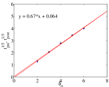
Figure 4.1: Reconnection times as a function of the initial separation. Reconnection times are estimated by using times immediately before and after reconnection plus the empirical 1/3 and 2/3 scaling laws.

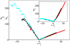
Figure 4.2: Pre- and post-reconnection separations for four cases: $\delta_{0}=2,3,4,5,6$ for calculations with $256^{3}$ points. ${\color[rgb]{0,0,1}\bf\bullet}$: $\delta_{0}=2$, ${\color[rgb]{0.31,1,0.5}\bf+}$: $\delta_{0}=3$, ${\color[rgb]{1,0,0}\bigcirc}$: $\delta_{0}=4$, ${\bf\divideontimes}$: $\delta_{0}=5$, ${\color[rgb]{0,1,1}\triangle}$: $\delta_{0}=6$. Pre-reconnection distances are raised to the power 3, while post-reconnection distances are raised to the power 3/2. This scaling is visibly better than the dimensional prediction ($\delta^{2}$ versus time to reconnection) shown in the inset. The scaled separations for $t<t_{r}$ fluctuate more strongly than the $t>t_{r}$ scaled separations.

4.2 Sub-Berloff profile.

Why was it necessary to use the sub-Berloff profile? That is, could a different profile give similar separation collapse for all the $\delta_{0}$ cases and obtain clear scaling laws, as in figure 4.2? To show the benefits of the sub-Berloff profile, tests were done using all of the known Padé approximate profiles of steady-state two-dimensional quantum vortices in an infinite domain, including tests with and without adding the mirror images. This included, the true Berloff profile, that is (2.7) with $c_{2}=d_{2}=0.02864$, the low-order $2\times 2$ Padé approximate of the Fetter (1969), (2.7) with $d_{1}=1$ and $c_{2}=d_{2}=0$, and a variety of $3\times 3$ Padé approximates from Berloff (2004) and most recently Rorai et al. (2013), solutions that are very close to the ideal diffusive solution. All gave roughly the same oscillations in the approach and separation curves as in Zuccher et al. (2012) and only a hint of the clear scaling laws in figure 4.2. Only the sub-Berloff profile with at least some of the mirror images worked. Further work will be needed to identify why instabilities generated on the vortex lines are either suppressed by the sub-Berloff profile, or absorbed by it.

4.3 Evolution of the orthogonal geometry during reconnection

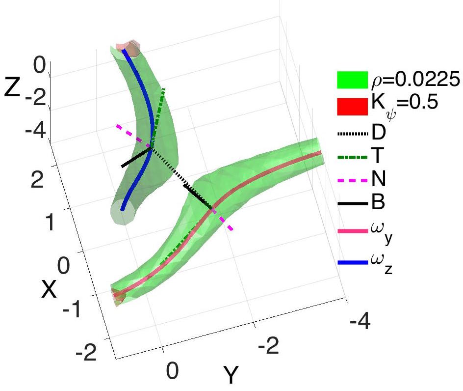
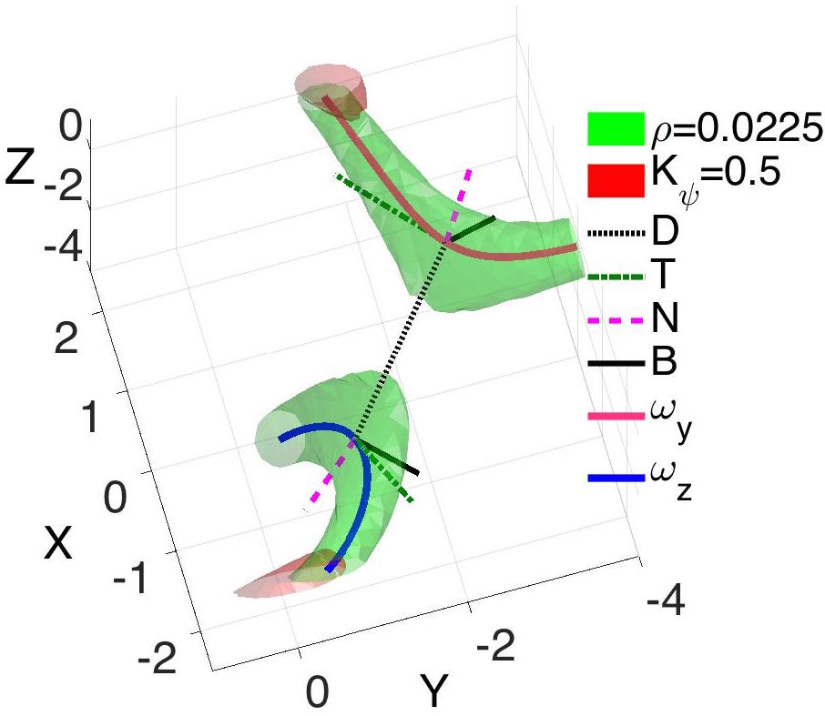
Figure 4.3: Isosurfaces, quantum vortex lines and orientation vectors in three-dimensions for the $\delta_{0}=3$, $256^{3}$ calculation at $t=6$ (4.4a), $t=8.75$ (4.4b) and $t=12$ (4.4c) where $t_{r}\approx 8.9$. Lines and vectors at the closest points on each vortex are the separation $D$ and Frenet-Serret vectors (3.3): $T$, $N$ and $B$.

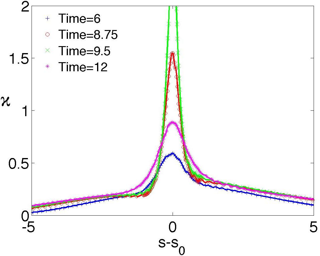
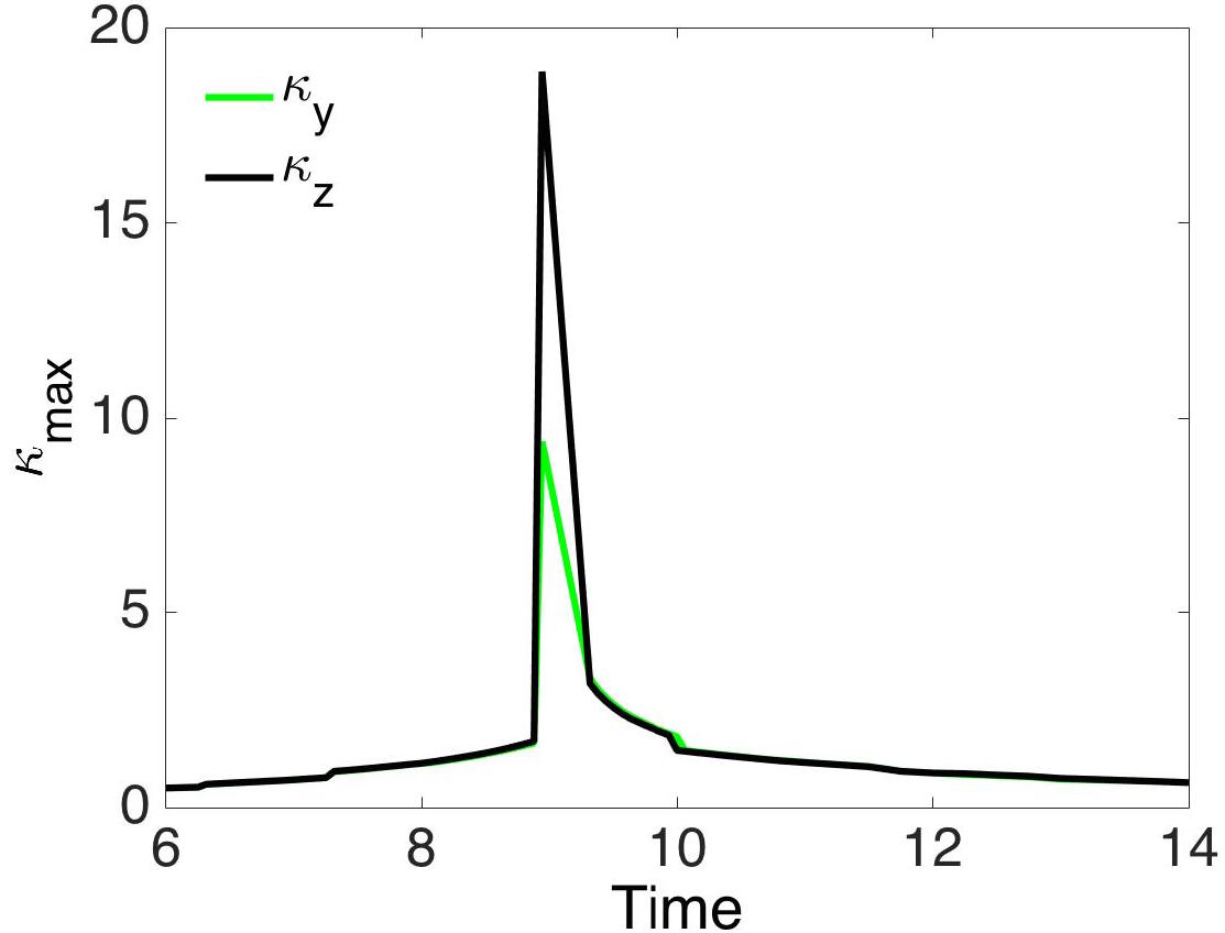
Figure 4.4: Curvature of the vortex lines is given only for the $\delta_{0}=3$ $256^{3}$ calculation with $t_{r}\approx 8.9$ as the curves about $t_{r}(\delta_{0})$ are similar for all $\delta_{0}$. (a) Curvatures against arclength $s$ at four times: $t=6$, 8.75, 9.5 and 12. The profiles for the other line are similar, with their maximum peaks at $t=9.5$ both off the plotted scale. (b) Time evolution of the maximum curvatures of the two lines. For each line there is a sudden jump to the large post-reconnection maximum at $t=t_{r}$.

The three-dimensional evolution of the vortices is illustrated in figures 2.3, 2.3 and 4.4 and the alignments at or near reconnection are illustrated with two sketches taken from different perspectives in figures 4.6 and 4.6. The purpose of the sketches is to emphasize the strong qualitative differences between the orthogonal reconnection’s skew-symmetric alignment and the anti-parallel case with its planar symmetries. Quantitative alignments are then given in figures 4.7, 4.8 and 4.9. This initial discussion is divided into three parts. First, the choice of three-dimensional images. Second, the role of the sketches. Third, how to use your fingers to put the pieces together into a mental picture.

Choice of 3D images. Section 2.2 uses figures 2.3 and 2.3 to illustrate the global changes in structure from two perspectives. One is a general perspective and the other is the Nazarenko perspective that shows the symmetries. Each figure has a $t=6$ frame, long before the reconnection at $t_{r}=8.9$, and a frame at $t=14$, long after reconnection.

Figure 4.4 focuses upon the reconnection zone using three times: $t=6$ is at the beginning of reconnection, $t=8.75$ is just before the reconnection time of $t_{r}\approx 8.9$ and $t=12$ shows the end of reconnection. Over this period the $\rho=0.05$ isosurfaces change slowly while the $\rho\equiv 0$ pseudo-vorticity lines within them move rapidly towards one another. The Frenet-Serret frames around the points of closest approach are discussed in subsections 4.4 and 4.5.

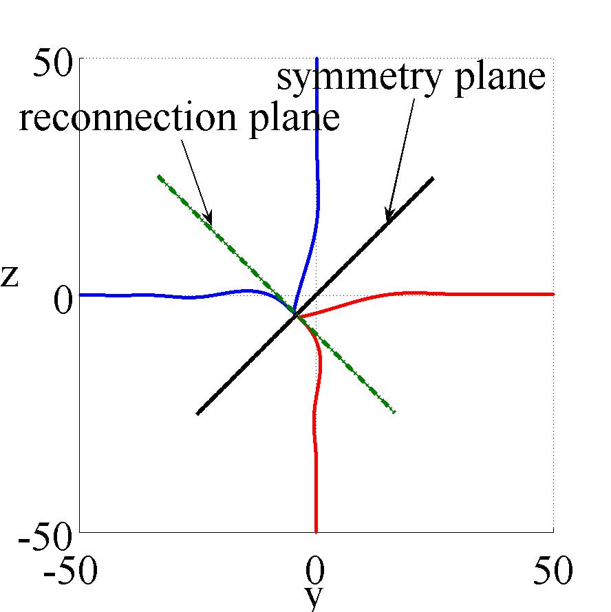
Figure 4.5: Sketch of the orthogonal reconnection around the reconnection point ${\bf x}_{r}$ at the reconnection time $t_{r}$ of the vortices projected onto the $y-z$ plane. The pre-reconnection trajectories approximately follow the $y-y_{mid}=0$ and $z-y_{mid}=0$ axes and the post-reconnection trajectories are the red and blue lines. Two projected planes are indicated in black. The reconnection plane $(z-z_{r})=-(y-y_{r})$ contains the tangents to the vortex lines $\mbox{\boldmath$T$}_{y,z}$ and their curvature vectors $\mbox{\boldmath$N$}_{y,z}$ both before and after reconnection, as well at the separation vector between the closest points $\mbox{\boldmath$x$}_{y,z}$. The propagation/symmetry plane $(z-z_{r})=(y-y_{r})$ which contains the bi-normals $\mbox{\boldmath$B$}_{y,z}$ and the direction of propagation of the mid-point $\mbox{\boldmath$x$}_{r}(t)$ between the closest points of the vortices: $\mbox{\boldmath$x$}_{y}$ and $\mbox{\boldmath$x$}_{z}$. From this perspective the angles along the reconnection plane before reconnection are shallow, and those after reconnection are sharp.

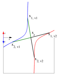
Figure 4.6: Sketch using the Nazarenko perspective, that is looking down on the reconnection plane along the propagation/symmetry plane, just before reconnection. Four line segments (in three-dimensions) have been added that connect $\mbox{\boldmath$x$}_{r}$, the mid-point between the vortices at closest approach, to four points, each located $\Delta s$ units along the vortices from their respective closest points. Angles generated between adjacent segments as a function of $\Delta s$ are plotted in figure 4.9.

Sketches: 2D and 3D. Figures 4.6 and 4.6 provide two planar sketches at or near the reconnection time, with the best reference point for each being the mid-point between the closest points on the two vortices:

$$\mbox{\boldmath$x$}_{r}(\delta_{0},t)=0.5(\mbox{\boldmath$x$}_{y}(t)+\mbox{\boldmath$x$}_{z}(t))\,.$$ (4.1)

The sketch in figure 4.6 projects the vortices at the reconnection time $t_{r}$ onto the $y-z$ plane around the point of reconnection: $\mbox{\boldmath$x$}_{r}(\delta_{0},t_{r})$, along with projections of two planes of interest, the reconnection or osculating plane and the propagation/symmetry plane, which are defined in terms of the average Frenet-Serret basis vectors (4.2) in subsection 4.5. The second sketch in figure 4.6 looks down the $x=0$, $y=z$ 45^∘ direction of propagation of $\mbox{\boldmath$x$}_{r}(\delta_{0},t)$ onto the $\mbox{\boldmath$T$}_{av}\times\mbox{\boldmath$N$}_{av}$ (4.2) reconnection plane. Important features include:

• Because figure 4.6 is at $t=t_{r}$, the projections of the planes and vortices all cross at $\mbox{\boldmath$x$}=\mbox{\boldmath$x$}_{r}(\delta_{0},t_{r})$, which means that the red and blue curves trace both the pre- and post-reconnection trajectories of the vortices, as follows:

  • The trajectories before reconnection follow the curves parallel to the $y=0$ and $z=0$ axes that are half blue and half red. These are projections of the red and blue lines in figure 4.6.

  • The trajectories immediately after reconnection are indicated by the red and blue curves coming out of the reconnection plane.

• The two orthogonal lines through $\mbox{\boldmath$x$}_{r}$ represent two planes:

  • The reconnection plane, defined by $\mbox{\boldmath$T$}_{av}=0.5(\mbox{\boldmath$T$}_{y}-\mbox{\boldmath$T$}_{z})$ and $\mbox{\boldmath$N$}_{av}=0.5(\mbox{\boldmath$N$}_{y}-\mbox{\boldmath$N$}_{z})$ (4.2). Before or after reconnection, the separation vector $\mbox{\boldmath$D$}=(\mbox{\boldmath$x$}_{z}-\mbox{\boldmath$x$}_{y})/|\mbox{\boldmath$x$}_{z}-\mbox{\boldmath$x$}_{y}|\neq 0$ is also in this plane.

    • It is shown below that $\mbox{\boldmath$T$}_{y,z}$ and $\mbox{\boldmath$N$}_{y,z}$ swap at reconnection, so all of these basis vectors stay in this plane after reconnection.

  • And the propagation plane, which contains the velocity of $\mbox{\boldmath$x$}_{r}(\delta_{0},t)$ and the average bi-normal $\mbox{\boldmath$B$}_{av}=0.5(\mbox{\boldmath$B$}_{y}+\mbox{\boldmath$B$}_{z})$ (4.2).

• The $x=0$, $y=z$ projection in figure 4.6 is denoted the Nazarenko perspective or NP because it was used by linear model of Nazarenko & West (2003).

  • That model tells us that $\mbox{\boldmath$x$}_{r}=0.5(\mbox{\boldmath$x$}_{y}+\mbox{\boldmath$x$}_{z})$ translates in the $(-y,-z)$ direction, motion that implies that the reconnection does not occur at the centre of the computational box.

  • Note that for the points on either side of $\mbox{\boldmath$x$}_{r}$, the tangents $\mbox{\boldmath$T$}_{y,z}$ and curvature vectors $\mbox{\boldmath$N$}_{y,z}$ are anti-parallel. The components that are not anti-parallel are directed out of the Nazarenko perspective. This also holds for the lines across the central, green $\rho=0.05$ isosurface in figure 4.4b. figure 4.7a shows how $\mbox{\boldmath$T$}_{y}\cdot\mbox{\boldmath$T$}_{z}$, $\mbox{\boldmath$N$}_{y}\cdot\mbox{\boldmath$N$}_{z}$ and $\mbox{\boldmath$B$}_{y}\cdot\mbox{\boldmath$B$}_{z}$ converge to this state as $t\rightarrow t_{r}$.

  • The lines drawn across the centre of figure 4.6 are used to determine the long-range angles discussed in section 4.6.

• 3D by using fingers. Cross your index fingers while pointing their knuckles towards one another so they do not touch.

  • Rotating this configuration reproduces figures 2.3a, 2.3a and 4.4a.

  • Now move your fingers up, bending them as you do and bringing the knuckles together.

  • This is how, the alignments of the Frenet-Serret frames at the points of closest approach in figure 4.7 form.

  • Now hold that configuration and rotate it to get the configurations of the sketches in figures 4.6 and 4.6 and the three-dimensional images in figures 2.3b, 2.3b and 4.4b.

4.4 Curvature

Curvature, has played a central role in our understanding of quantum turbulence due to its use in predicting velocities in the law of Biot-Savart and the local induction approximation. The connection between these approximations for the velocities and the true dynamics of quantum fluids, as modeled by the Gross-Pitaevskii equations, would be in how the gradient of the phase $\phi$ of the wavefunction $\psi$ is modified by the curvature of the vortex lines.

In that context, could curvature profiles provide clues for the origins of the anomalous scaling exponents of the orthogonal separations? For example, if the local induction approximation is relevant, then a sudden increase in the maximum curvature of the lines could explain the change in scaling.

To assess whether this is a possible explanation, figure 4.4 plots profiles of the curvature along the vortex lines at several times, and the curvature maxima $\kappa_{\rm max}$ as a function of time for the $\delta_{0}=3$ case. The other cases have similar behaviour, including one slightly under-resolved $\delta_{0}=4$ case in a large $(32\pi)^{3}$ domain.

Two primary features should be noted. First, in figure 4.4a there is very little asymmetry in $s$ about the points of cloest approach, both before and after reconnection. Second, in figure 4.4b, there is some growth in $\kappa_{\rm max}$ for $t<t_{r}$, followed by a sharp jump in $\kappa_{\rm max}$ at $t=t_{r}$, which then relaxes rapidly to the pre-reconnection values of $\kappa_{\rm max}$.

So there is some qualitative support for a local induction explanation change between the $\delta_{in}$ and $\delta_{out}$ scaling, but there is also inconsistency with the following:

• Even pre-reconnection, the $\delta_{in}\sim(t_{r}-t)^{-1/3}$ scaling would require a stronger growth in $\kappa$ than is observed.

• Post-reconnection, and after the curvature spike has relaxed, stronger curvatures than are observed would be needed to maintain the $\delta_{out}\sim(t_{r}-t)^{-2/3}$.

Therefore, one must conclude that a bigger picture is needed. Our proposal is to look at the alignments of their respective Frenet-Serret frames as another reason for the changes in scaling. Looking first at the alignments of at the points of closest approach, then at distances away from those points (Rorai, 2012).

Another possible explanation, if the local induction approximation is relevant, would be if the curvature maxima are stronger post-reconnection. The inset in figure 4.4 does show that the maxima are slightly stronger post-reconnection, but this does not appear to be the whole story. To get a bigger picture we need to look beyond the curvature profiles and see how the vortices are aligned with each other for points along their entire trajectories. Starting with the alignments of their respective Frenet-Serret frames at the points of closest approach, then for distances away from those points.

4.5 Orthogonal: Frenet-Serret orientation.

Besides allowing us to calculate the curvature of the vortex lines, knowing their trajectories allows us to calculate the Frenet-Serret frame (3.3). This has been done for the $256^{3}$, $\delta_{0}=3$ calculation for all times and provides quantitative support for the describing the local frame at the reconnection point $\mbox{\boldmath$x$}_{r}$ in terms of the reconnection plane and the propagation plane indicated in figure 4.6.

Figures 4.7 and 4.8 show the following evolution of the Frenet-Serret frames at the closest points $\mbox{\boldmath$x$}_{y,z}$:

• For $t<t_{r}$, pre-reconnection:

  • figure 4.7a shows that the vorticity direction or tangent vectors $\mbox{\boldmath$T$}_{y,z}$, the curvature vectors $\mbox{\boldmath$N$}_{y,z}$ and the bi-normals $\mbox{\boldmath$B$}_{y,z}$ converge to their opposites as $t\rightarrow t_{r}$, both before and after reconnection.

  • figure 4.7b shows that $\mbox{\boldmath$T$}_{y,z}$, $\mbox{\boldmath$N$}_{y,z}$ and their unit separation vector $\mbox{\boldmath$D$}=(\mbox{\boldmath$x$}_{z}-\mbox{\boldmath$x$}_{y})/|\mbox{\boldmath$x$}_{z}-\mbox{\boldmath$x$}_{y}|$ all lie in the same plane, the reconnection plane in figure 4.6.

  • The bi-normals $\mbox{\boldmath$B$}_{y,z}$ define the propagation plane.

  • The useful averages of the Frenet-Serret frames between $\mbox{\boldmath$x$}_{y}$ and $\mbox{\boldmath$x$}_{z}$ are these:

    $$\begin{array}[]{clclc}\vskip 6.0pt plus 2.0pt minus 2.0pt\circ&\mbox{\boldmath$N$}_{av}&=&0.5(\mbox{\boldmath$N$}_{y}-\mbox{\boldmath$N$}_{z})&\quad\mbox{and is parallel to}~{}\mbox{\boldmath$D$}(t)\\ \vskip 6.0pt plus 2.0pt minus 2.0pt\circ&\mbox{\boldmath$T$}_{av}&=&0.5(\mbox{\boldmath$T$}_{y}-\mbox{\boldmath$T$}_{z})&\quad\mbox{and is perpendicular to both}~{}\mbox{\boldmath$N$}_{av}~{}{\rm and}~{}\mbox{\boldmath$D$}.\\ \vskip 6.0pt plus 2.0pt minus 2.0pt\circ&\mbox{\boldmath$B$}_{av}&=&0.5(\mbox{\boldmath$B$}_{y}+\mbox{\boldmath$B$}_{z})&\quad\mbox{and is perpendicular to}~{}\mbox{\boldmath$T$}_{av},~{}\mbox{\boldmath$N$}_{av}~{}{\rm and}~{}\mbox{\boldmath$D$}.\\ \end{array}$$ (4.2)

  • That is: Subtract the tangent and curvature vectors because they become anti-parallel as $t\nearrow t_{r}$, and add the bi-normals because they are parallel as $t\nearrow t_{r}$.

  • These alignments between $\mbox{\boldmath$T$}_{av}$, $\mbox{\boldmath$N$}_{av}$ and $\mbox{\boldmath$B$}_{av}$ with $D$ form in the early stages, long before the reconnection at $t_{r}=8.9$.

• The post-reconnection Frenet-Serret flip:

  • Figure 4.8 shows that the directions of $\mbox{\boldmath$T$}_{av}$ and $\mbox{\boldmath$N$}_{av}$ swap and $D$ rotates by 90^∘ so that all three are still in the reconnection plane with the same relations to one another.

  • $\mbox{\boldmath$B$}_{av}$ remains orthogonal to the reconnection plane.

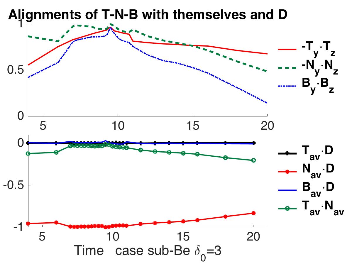
Figure 4.7: These two frames show how the basis vectors of the Frenet-Serret frames (3.3) at the closest points $\mbox{\boldmath$x$}_{y,z}$ of the $\delta_{0}=3$, $256^{3}$ calculation are aligned and help define the reconnection plane and the propagation plane used in figures 4.6 and 4.6. a): The alignments between the Frenet-Serret components at $\mbox{\boldmath$x$}_{y,z}$. For $t<t_{r}$ the tangent vectors $\mbox{\boldmath$T$}_{y,z}$ and curvature vectors $\mbox{\boldmath$N$}_{y,z}$ become increasingly anti-parallel as the reconnection time is approached while the bi-normal vectors $\mbox{\boldmath$B$}_{y,z}$ become increasingly aligned. These trends are are reversed for $t>t_{r}$. b): The alignments between the averages over $\mbox{\boldmath$x$}_{y,z}$ of the Frenet-Serret frames defined by (4.2) with the separation vector $D$ between $\mbox{\boldmath$x$}_{y}$ and $\mbox{\boldmath$x$}_{z}$.

Figure 4.8: For the $\delta_{0}=3$, $256^{3}$ calculation, the alignments over time of $\mbox{\boldmath$D$}(t_{r}^{-})=\mbox{\boldmath$D$}(t_{r}-dt)$ with $\mbox{\boldmath$T$}_{av}$ and $\mbox{\boldmath$N$}_{av}$, the averages (4.2) over the tangent and curvature components of the Frenet-Serret frames at the closest points $\mbox{\boldmath$x$}_{y,z}$. $\mbox{\boldmath$B$}_{av}\cdot\mbox{\boldmath$D$}(t_{r}^{-})\approx 0$ for all times. $\mbox{\boldmath$D$}(t_{r}^{-})$ is the separation direction at $t=8.9$, just before reconnection.

The alignments of the components of the Frenet-Serret frames at $\mbox{\boldmath$x$}_{y,z}$ and the separation of these points $D$ is significantly different than their alignments for the anti-parallel case in Sec. 5. Comparisons are discussed in the Summary in Sec. 6.

4.6 Angles at reconnection

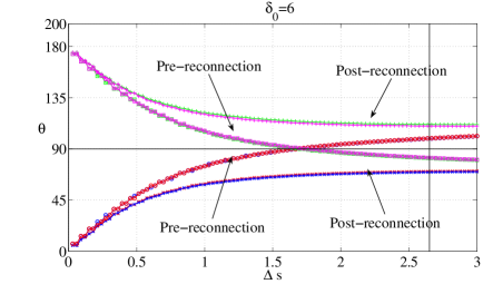
Figure 4.9: Angles between the segments in 3D space displayed in figure 4.6 as a function of $\Delta s$ for $\delta_{0}=6$ and $t=63$ (pre-reconnection) and $t=65$ (post-reconnection). The angles between the arms of the same vortex, triplets [$\mbox{\boldmath$x$}_{1,v1},~{}\mbox{\boldmath$x$}_{r},~{}\mbox{\boldmath$x$}_{2,v1}$] and [$\mbox{\boldmath$x$}_{1v2},~{}\mbox{\boldmath$x$}_{r},~{}\mbox{\boldmath$x$}_{2v2}$], are indicated by circles (blue and red) before reconnection, and stars (blue and red) after reconnection. The angles sum to 360^∘ as $\Delta s\rightarrow 0$, implying that the segments near the reconnection point $\mbox{\boldmath$x$}_{r}$ lie on a plane, specifically, the reconnection plane in figure 4.6 The sum of the angles grows with $\Delta s$ and is about $\sim 362^{\circ}$ for $\Delta s\sim 2.6$ (vertical black line), which is consistent with the arms of reconnecting vortices becoming progressively more convex and hyperbolic as they move away from $\mbox{\boldmath$x$}_{r}$, both before and after reconnection. The rapidly changing behavior for small $\Delta s$ is a kinematic result of how the lines and angles indicated in figure 4.6 were chosen and is not significant. What could be more significant are the differences in the angles for intermediate $\Delta s$ and their influence upon any Biot-Savart contributions to the velocities.

What additional dynamics might help us identify the differences between the orthogonal and anti-parallel separation scaling laws?

One place to look is larger-scale alignments and long-range interactions. While the underlying Gross-Pitaevskii equations are local, the existence of the vortex structures means that such alignments should exist and should influence the local motion of the $\rho\equiv 0$ lines to the degree that the law of Biot-Savart can be applied. With the goal of identifying any such long-range interactions, this section determines the evolution of pre- and post-reconnection angles between points on the extended structures.

Relevant angles can be defined between the arms of the reconnecting vortices around the reconnection point as follows.

• From the points of closest approach $\mbox{\boldmath$x$}_{y,z}(t)$, define $\mbox{\boldmath$x$}_{r}(t)=0.5(\mbox{\boldmath$x$}_{y}(t)+\mbox{\boldmath$x$}_{z}(t))$.

• Move $\pm\Delta s$ along the arms of the vortices from $\mbox{\boldmath$x$}_{y,z}(t)$ and identify four new points: ${\bf x}_{1,y}$, ${\bf x}_{2,y}$, ${\bf x}_{1,z}$ and ${\bf x}_{2,z}$, illustrated in the Nazarenko perspective sketch in figure 2.3

• To get a fully three-dimensional perspective, note that these points lie on outstretched arms such as in figure 2.3b.

• Connect the four points with ${\bf x}_{r}$ to form an extended three-dimensional frame then calculate the angles $\theta_{i}$ between these four vectors.

• Plots of $\theta_{i}(\Delta s)$ show qualitatively similar variations independent of $\delta_{0}$ with these properties:

  • The sum of the $\theta_{i}$ grows as $\Delta s$ increases, starting from $\sum_{i}\theta_{i}(\Delta s=0)=360^{\circ}$.

  • This shows that the inner ($\Delta s\approx 0$) structure is a plane.

  • The vertical line in figure 4.9 represents the $\Delta s_{p}$ for which $\sum_{i}\theta_{i}(\Delta s)=362^{\circ}>360^{\circ}$, indicating that the structure is mildly hyperbolic.

  • $\sum_{i}\theta_{i}(\Delta s)$ increases with $\Delta s$, implying that the global structure is convex or hyperbolic, the opposite of a structure with an acute angles such as a pyramid.

  • The primary quantitative difference as $\delta_{0}$ decreases is that the $\theta=90^{\circ}$ pre-reconnection cross-over, at $\delta s=1.5$ for $\delta_{0}=6$, decreases.

  • In addition, the geometry becomes more hyperbolic. That is $\sum_{i}\theta_{i}(\Delta s)$ increases as $\delta_{0}$ decreases with $\sum_{i}\theta_{i}(\Delta s)=370^{\circ}$ for$\delta_{0}=3$.

  • The inner angles, that is the angles between the triplets [$\mbox{\boldmath$x$}_{1,v1},~{}\mbox{\boldmath$x$}_{r},~{}\mbox{\boldmath$x$}_{2,v1}$] and [$\mbox{\boldmath$x$}_{1v2},~{}\mbox{\boldmath$x$}_{r},~{}\mbox{\boldmath$x$}_{2v2}$], are larger than 90^∘ before reconnection and smaller after. The difference is about 20^∘ in all of the calculations and would be consistent with the observed slower approach and faster separation.

  • When looking down at the reconnection plane in either figures 4.6 or figure 2.3b, do not forget that the centre of the reconnection plane is moving along the $y=z$ direction of the propagation plane and simultaneously dragging or pushing the extended arms as it moves, as in figure 2.3b.

Understanding these features could provide us with some hints about the origins of the anomalous scaling laws. One hint could be the different angles at intermediate scales, $0.5\leq\Delta s\leq 2.5$. Pre-reconnection, the this span has approximately retained its original $\theta\sim 90^{\circ}$ orthogonal alignment. Post-reconnection the angles over this span still sums to approximately $362^{\circ}$ degrees, but the angles on either side of the reconnection have jumped by $\pm 20^{\circ}$. The sudden jump is due to how the directions of the tangent and curvature vectors swap at reconnection. Using the sketch in figure 4.6, this means that prior to reconnection the angle in 3D space is between the triplets [$\mbox{\boldmath$x$}_{1,v1},~{}\mbox{\boldmath$x$}_{r},~{}\mbox{\boldmath$x$}_{2,v1}$] and [$\mbox{\boldmath$x$}_{1v2},~{}\mbox{\boldmath$x$}_{r},~{}\mbox{\boldmath$x$}_{2v2}$] and afterwards between the triplets [$\mbox{\boldmath$x$}_{1v1},~{}\mbox{\boldmath$x$}_{r},~{}\mbox{\boldmath$x$}_{1v2}$] and [$\mbox{\boldmath$x$}_{2v1},~{}\mbox{\boldmath$x$}_{r},~{}\mbox{\boldmath$x$}_{2v2}$]. Similar behaviour is seen for all the $\delta_{0}$ cases. It is visualised for $\delta_{0}=3$, using two perspectives in figures 2.3 and 2.3.

To goal is find a model that links the sudden swaps in local alignments in figures 4.7 and 4.8 with the nonlocal changes in figure 4.9 and from that explains the anomalous orthogonal reconnection scaling. This model must also accommodate the scaling of anti-parallel reconnection, which obeys the expected dimensional scaling both before and after reconnection. The final discussion in section 7 addresses what might be required.

5 Anti-parallel results: approach, separation, curvature

In contrast to the orthogonal vortices, whose scaling laws do not obey expectations, it will now be shown that the scaling of initially anti-parallel vortices obeys those expectations almost completely.

Figure 2.1 illustrated the overall structure of our anti-parallel case before reconnection at $t=0.125$ and after reconnection at $t=4$, where $t_{r}\approx 2.44$. The very low density $\rho=0.05$ isosurface is the primary diagnostic for the vortex lines and as in Kerr (2011), the post-reconnection density isosurfaces are developing a second set of reconnections near $y=\pm 5$ from which the first set of vortex rings will form. Eventually two stacks of vortex rings on either side of $y=0$ should form from the additional waves along the original vortex lines. Large values of the gradient kinetic energy (2.4) and the magnitude of the pseudovorticity (3.1) are shown using two additional isosurfaces and the trajectories of the $\rho\approx 0$ pseudo-vorticity are traced with thick lines.

Figure 5.1 provides two perspectives of the structure approximately at the reconnection time using the same isosurfaces and vortex lines as in figure 2.1, except there are now two sets of vortex lines. figure 2.1a shows two red curves seeded using $\rho\approx 0$ points on the $y=0$, $x-z$ perturbation plane and two blue curves seeded using $\rho\approx 0$ points on the $z=0$, $x-y$ dividing plane, representing respectively the pre- and post-reconnection trajectories.

As for the $\delta_{0}=3$ orthogonal case in figure 4.4b, the reconnection time isosurfaces have an extended zone of very low density around the reconnection point and a strong isosurface of the gradient kinetic energy outside this zone. Large values of $|\omega_{\rho}|$ are also outside the reconnection zone.

Figure 5.1: Density, kinetic energy $K_{\psi}=0.5|\nabla\psi|^{2}$ (2.4) and pseudo-vorticity $|\nabla\psi_{r}\times\nabla\psi_{i}|$ isosurfaces plus vortex lines a bit after the time of the first reconnection, $t=2.4375\gtrsim t_{r}=2.344$ from two perspectives with $\max(K_{\psi})=0.83$. $\max|\omega_{\rho}|=0.4$ for all the times. (a) shows four vortex lines, with each pair starting at the points of nearly zero density on the $y=0$ and $z=0$ symmetry planes respectively. (b) gives a second perspective that looks into a quadrant through the two symmetry planes and is designed to demonstrate that locally, around $y=z=0$, the shape of the $\rho=0.05$ isosurface is symmetric on the two symmetry planes.

Figure 5.2 presents several possible fits for the pre- and post-reconnection separation scaling laws, with both the pre-reconnection incoming and post-reconnection outgoing separations following the predicted dimensional scaling of $\delta\sim|t_{r}-t|^{1/2}$ (1.1), unlike the orthogonal cases just shown. Furthermore, for $\Delta t=|t-t_{r}|<0.5$, the $\delta_{\rm in}(t_{r}-t)$ and $\delta_{\rm out}(t_{r}-t)$ are almost mirror images of each other. Although that is not the case for larger $\Delta t$.

This suggests that unlike the orthogonal case, where we have attempted to relate the asymmetric scaling laws to asymmetries in the underlying structure, for the anti-parallel case we want to identify physical symmetries that would predispose the scaling laws to be temporally symmetric and follow the dimensional prediction.

The purpose of giving two perspectives near the reconnection time in figure 5.1 is to clarify the physical symmetries at this time. The overall structure in figure 5.1a shows how all four legs of vorticity converge on the $y=z=0$ line where the $x-z$ or $x-y$ symmetry planes cross. Then figure 5.1b looks at the structure from the interior of the zone of nearly zero density from the perspective of the $\rho\approx 0$, $y-z$ reconnection plane upon which the vortices reconnect. In a manner analogous to when the orthogonal vortices reconnect in figure 4.4, the tangent and normal vectors swap directions, with pre-reconnection tangent in $y$ becoming the post-reconnection normal, and the normal in $z$ becoming the tangent. This results in the butterfly trajectories around the $y=z=0$ line in figure 5.1a.

A useful, but not perfect, way to characterise the resulting structure is to use the proposal by de Waele & Aarts (1994), based on their Biot-Savart calculation of anti-parallel quantum vortices, that near reconnection the vortices form an equilateral pyramid. The pyramid for figure 5.1a can be formed by straightening the 2 red and 2 blue curved legs of vorticity surrounding the $y=z=0$ line in $x$ to $(x,y,z)\approx(18,0,0)$, slightly to the left of the $\rho=0.05$ isosurface. These extensions would start from tangents to the red and blue lines. The angles $\theta_{yz}$ of these tangents with respect to the symmetry planes would define the sharpness of the tip of pyramid and depend on where the tangents are taken from. $\theta_{y,z}=45^{\circ}$ is obtained for $|y|=|z|\leq 2$, which is where the vortices begin to bend back upon themselves.

Why don’t the pseudo-vortex lines continue to bend, or kink, until a sharp tip with $\theta_{y,z}=45^{\circ}$ is obtained? Figure 5.3 provides the clues by directly plotting the curvatures and the inclinations of the tips of the $y$ and $z$ pseudo-vortex lines, which are the points of closest approach in figure 5.3a. The curvatures are determined by (3.4) and the inclinations come from $\mbox{\boldmath$N$}=(n_{x},n_{y},n_{z})$, the direction of the curvature from (3.3b). Independent of whether one considers the red $y$-vortices or blue $z$-vortices, their maximum curvatures have nearly the same upper bounds and the same maxima as $n_{y,z}/n_{x}$, with

$$\begin{array}[]{cl}n_{z}/n_{x}\nearrow 6\quad{\rm as}~{}~{}t\nearrow t_{r}&\quad{\rm for}~{}~{}t>t_{r}\quad{\rm and}\\ n_{y}/n_{x}\searrow 6\quad{\rm as}~{}~{}t\searrow t_{r}&\quad{\rm for}~{}~{}t_{r}>t\,.\end{array}$$ (5.1)

$\tan\theta_{\pm}=6$ corresponds to $80^{\circ}$, not the $45^{\circ}$ angles of a pyramid.

This means that as reconnection is approached, the direction of the curvature $N$ begins to be parallel to their separation $D$, very reminiscent of what has been found for the orthogonal vortices as $t\rightarrow t_{r}$ in figures 4.7 and 4.8. Which also means that the directions of the curvature and tangents nearly swap during reconnection, which is also similar to, but not exactly the same as, the orthogonal cases. And not what a true pyramid with a sharp tip would do.

What is probably more important for getting the dimensional scaling for $\delta(t)$ is that both sets of curves are temporally symmetric. That is, $\kappa(t_{r}-t)\approx\kappa(t-t_{r})$ and $n_{z}(t_{r}-t)/n_{x}(t_{r}-t)\approx n_{y}(t-t_{r})/n_{x}(t-t_{r})$. Figure 5.3b emphasises this further by showing the dependence of $\kappa_{y}$ and $\kappa_{z}$ on their arclengths $s$ at times just before and after the estimated reconnection time of $t_{r}=2.34$.

Finally, let us go back to the three-dimensional structures. First, consider how the $t<t_{r}$ vortex lines in figure 2.1a evolve into the pinched red $y$-vortex lines in figure 5.1a along a path in the $x-z$ symmetry plane with $(n_{x},0,n_{z})(t)=(\cos\theta_{-},0,\sin\theta_{-})\nearrow(\cos 80^{\circ},0,\sin 80^{\circ})$. Then note that the process is reversed for $t>t_{r}$ as the pinch in the blue $z$-vortex lines relaxes in $z$ as $\delta_{+}\searrow 0$ along a path in the $x-z$ symmetry plane from its most extreme orientation: $(n_{x},n_{y},0)(t)=(\cos\theta_{+},\sin\theta_{+},0)\searrow(\cos 80^{\circ},\sin 80^{\circ},0)$. Therefore the evolution of the in and out angles is temporally symmetric, as hoped for, even though the tip is not a true pyramid (5.1).

These results differ from the anti-parallel case in Zuccher et al. (2012), which shows a slower approach and faster separation, similar to the scaling observed for a recent anti-parallel Navier-Stokes calculation (Hussain & Duraisamy, 2011). There could be several reasons for the differences. First, the initial perturbations to the anti-parallel trajectories in Zuccher et al. (2012) are pointed towards one another, and not in the direction of propagation as here. Another difference is that their periodic boundaries in $y$ (the vortical direction) are relatively close, unlike that direction here. In Kerr (2011) and in a recent set of Navier-Stokes reconnection calculations Kerr (2013), the advantages of making that direction very long have already been discussed.

Figure 5.2: Separations near the time of the first reconnection of the anti-parallel vortices. The positions are found using the isosurface method on the symmetry planes. Both pre- and post-reconnection curves (in and out) follow $\delta_{0}\sim(t_{r}-t)^{1/2}$ most closely.

Figure 5.3: a: Maximum curvatures, $\kappa_{y0}$, $\kappa_{z0}$, versus time. $\kappa_{y0}$ and $\kappa_{z0}$ are always on symmetry planes. The approach before reconnection and separation after reconnection are similar. Reconnection time is where the curves cross, $t_{r}\approx 2.344$. b: Curvatures as a function of arclength along the vortices near the reconnection time, with the profile from the new $z$ vortex taken a bit before $t_{r}$ and the profile of the old $y$ vortex a bit after $t_{r}$. The curavatures near $y=z=0$ are similar, which drives similar approach and separation velocities.

6 Summary

The reconnection scalings of two configurations of paired vortices, orthogonal and anti-parallel, have been found to have different scaling exponents.

For the anti-parallel case, the temporal scaling of both the pre- and post-reconnection separations obey the dimensional prediction, $\delta_{\pm}(t)\sim A\sqrt{\Gamma|t_{r}-t|}$ and the arms of the vortex pairs as the reconnection time is approached form an equilateral pyramid with a smooth tip, which is in most respects qualitatively similar to the prediction of a Biot-Savart model (de Waele & Aarts, 1994). Around the smooth tip the curvatures $N$ and separation $D$ are nearly parallel and as a result the directions of curvature $N$ and the tangents $T$ almost swap during reconnection.

The orthogonal cases, in contrast, show asymmetric temporal scaling with respect to the reconnection time $t_{r}$. For $t<t_{r}$, $\delta_{-}(t)\sim A_{-}(\Gamma|t_{r}-t|)^{1/3}$ and for $t>t_{r}$, $\delta_{+}(t)\sim A_{+}(\Gamma|t_{r}-t|)^{2/3}$, where the coefficients $A_{\pm}$ are independent of the initial separation $\delta_{0}$. At $t\approx t_{r}$, the reconnecting vortices are anti-parallel, with the vortices interacting in a reconnection plane that contains the tangent and curvature vectors of both vortices as well as their separation vector. This results in the directions of curvature and vorticity swapping during reconnection.

Two innovations There are two innovations that allow these calculations to generate clean scaling laws. One is an initial core profile that either minimises the formation of secondary waves by the interacting vortices, or absorbs these waves. The second innovation is a way to trace the vortex lines that minimises the need to identify computational cells with small values of the density.

6.1 Contrasting geometries

While this paper has emphasised the differences between the reconnection scaling for the orthogonal and anti-parallel cases, a few similarites need to be noted when $t\approx t_{r}$ and $\mbox{\boldmath$x$}\approx\mbox{\boldmath$x$}_{r}$. That is within the reconnection zone in both time and space. First, within this zone the curvature vectors in both cases tend to align with the separation between the vortices and the opposing vortices are anti-parallel. The skew-symmetric alignment of the reconnecting orthogonal vortices seems to be sufficient for imposing this local property. Post-reconnection, in both cases the curvature and tangent directions swap, or nearly so in the anti-parallel case.

This also means that in neither case does a pyramid form in the zone immediately around $\mbox{\boldmath$x$}_{r}$. Nor do any of the fixed point solutions identified in Meichle et al. (2012) form.

However, further from $\mbox{\boldmath$x$}_{r}$, the situation is different. For the orthogonal cases, angles between the vortices imply a convex or hyperbolic structure. In the anti-parallel case, a pyramid forms with nearly acute angles.

Let us summarise the additional key features of the orthogonal cases.

Orthogonal

From an early time, the closest points of the originally orthogonal vortices become locally anti-parallel and their respective curvature vectors become anti-aligned with the line of separation. Combined, this implies that the local bi-normals for each line are nearly parallel and do not point in the direction of separation. At reconnection, the directions of the vorticity and curvature swap, and the sign of the bi-normal reverses. All of this is in a reconnection plane defined by the averages of the curvature and vorticity directions at the points of closest approach.

Another useful perspective is the Nazarenko perspective in figure 2.3, which is along a 45^∘ angle in the $y-z$ plane. From this perspective, the vortices are always distinct, without any loops, and one can see that the pre-reconnection vortices approach the reconnection from one direction, and post-reconnection vortices separate in another. This perspective is used for finding non-local alignments and angles as in figure 4.9, which show that the global alignment of the initial orthogonal vortices is hyperbolic.

While the three-dimensional graphics for our orthogonal cases are qualitatively similar to the equivalent Gross-Pitaevskii density isosurfaces in Zuccher et al. (2012), our interpretation of the underlying geometry is different. Zuccher et al. (2012) conclude that the deviations of Gross-Pitaevskii separations from the dimensional prediction is only near the reconnection and probably due to the rarefaction waves they report. In contrast, our analysis shows that the derivations start much before that and continue until the reconnection time. Furthermore, this local scaling appears to be a result of the global alignment that exists for almost all times.

Our conclusion is that the new scaling laws appear at all times for initially orthogonal vortices and these scaling laws are probably tied to the unique alignment of the Frenet-Serret frames that form early and continue through the reconnection period until to the end of each calculation. That these anomalous scaling laws are identical, about their respective reconnection times, for all initial separations, implies that the anomalous scaling laws could exist for initial vortices with macroscopic initial separations extending to observable scales.

7 Discussion

These results leave us with several major questions.

• First, could the scaling laws shown here be extended to the huge range of length scales in experiments? Because the new orthogonal scaling laws appear at all times for initially orthogonal vortices and these scaling laws are tied to unique alignments that form early and continue through the reconnection period, it is possible that the anomalous scaling could apply to vortices on the macroscopic, observable scales.

  However, what if the initial state is not strictly orthogonal? What seems to be true, based upon several additional curved configurations considered in Rorai (2012) as well as cases from Zuccher et al. (2012), is that the scaling of all quantum reconnection events should lie between the two extremes presented here. More work will be needed to determine when and for how long each type of scaling dominates.

• Second, can these cases be compared with the experiments using solid hydrogen markers? Improvements in both the experimental and numerical data sets will be needed before that can be addressed properly. Currently, a few isolated events in some of the experimental videos and the first experimental paper (Bewley et al., 2008) might be consistent with orthogonal scaling asymmetries described here. However, in the best statistical analysis (Paoletti et al., 2008), the distributions of the approaches and separations are clustered about the dimensional prediction, represented by our anti-parallel case.

• Finally, how can the alignments quantified here for the orthogonal cases be used to explain the anomalous reconnection scaling laws? The local swaps in the alignment of the Frenet-Serret frames for the orthogonal cases in figures 4.7 and 4.8 are probably too similar to the local swaps for the anti-parallel case in figure 5.3 to explain the non-dimensional scaling laws. So a better place to start might be to consider the large-scale alignments. However, to use these alignments together with Biot-Savart to predict velocities could lead nowhere since all of full Biot-Savart calculations find the dimensional, temporally symmetric scaling laws.

• Nonetheless, Biot-Savart can be a useful place to start looking in the sense that (3.2) provides us with a means to exactly determine the Gross-Pitaevskii velocities, which could then be compared to the Biot-Savart predictions. Once the differences have been identified, and from there the sources of these differences, we should be on the road to explaining this new behaviour.

References

- Berloff (2004) Berloff, N.G. 2004 Interactions of vortices with rarefaction solitary waves in a Bose-Einstein condensate and their role in the decay of superfluid turbulence Phys. Rev. A 69, 053601.
- Bewley et al. (2008) Bewley, G.P., Paoletti, M. S., Sreenivasan, K. R., & Lathrop, D. P. 2008 Characterization of reconnecting vortices in superfluid helium Proc. Nat. Aca. Sci. 105, 1370713710.
- Boratav et al. (1992) Boratav, O.N., Pelz, R.B., & Zabusky, N.J. 92 Reconnection in orthogonally interacting vortex tubes: Direct numerical simulations and quantification in orthogonally interacting vortices Phys. Fluids A 4, 581605.
- de Waele & Aarts (1994) de Waele, A.T.A.M, & Aarts, R.G.K.M. 1994 Route to vortex reconnection Phys. Rev. Lett. 72, 482485.
- Fetter (1969) Fetter, A. L. 1969 . In Lectures in Theoretical Physics: Quantum Fluids and Nuclear Matter, volume XIB (ed. K. T. Mahanthappa and W. E. Brittin), pp. 351-. Gordon & Breach Science Pub, New York.
- Kerr (2011) Kerr, R.M. 2011 Vortex stretching as a mechanism for quantum kinetic energy decay Phys. Rev. Lett. 106, 224501.
- Kerr (2013) Kerr, R.M. 2013 Swirling, turbulent vortex rings formed from a chain reaction of reconnection events Phys. Fluids 25, 065101.
- Koplik & Levine (1993) Koplik, J., & Levine, H. 1993 Vortex reconnection in superfluid helium Phys. Rev. Lett. 71, 13751378.
- Hussain & Duraisamy (2011) Hussain, F., & Duraisamy, K. 2011 Mechanics of viscous vortex reconnection Phys. Fluids 23, 021701.
- Leadbeater et al. (2001) Leadbeater, M., Winiecki, T., Samuels, D. C., Barenghi, C. F., & Adams, C. S. 2001 Sound Emission due to Superfluid Vortex Reconnections Phys. Rev. Lett. 86, 14101413.
- Leadbeater et al. (2003) Leadbeater, M., Samuels, D. C., Barenghi, C. F., & Adams, C. S. 2003 Decay of superfluid turbulence via Kelvin-wave radiation Phys. Rev. A 67, 015601.
- Meichle et al. (2012) Meichle, D.P., Rorai, C., Fisher, M.E., & Lathrop, D.P. 2012 Quantized vortex reconnection: Fixed points and initial conditions Phys. Rev. B 86, 014509.
- Nazarenko & West (2003) Nazarenko, S., & West, R. 2003 Analytical solution for nonlinear Schrödinger vortex reconnection J. Low Temp. Phys. 132, 1–10.
- Paoletti et al. (2008) Paoletti, M. S., Fisher, M. E., Sreenivasan, K. R., & Lathrop, D. P. 2008 Velocity statistics distinguish quantum from classical turbulence Phys. Rev. Lett. 101, 154501.
- Rorai (2012) Rorai, C. 2012 Vortex reconnection in superfluid helium. University of Trieste.
- Rorai et al. (2013) Rorai, C., Sreenivasan, K. R., & Fisher, M. E. 2013 Propagating and annihilating vortex dipoles in the Gross-Pitaevskii equation Phys. Rev. B 88, 134522.
- Rorai et al. (2014) Rorai, C., J. Skipper, R.M. Kerr & K.R.Sreenivasan: 2014 Approach and separation of quantum vortices with balanced cores. arXiv:1410.1259v1.
- Sasa et al. (2011) Sasa, N., Kano, T., Machida, M., L’vov, V.S., Rudenko, O., & Tsubota, M. 2011 Energy spectra of quantum turbulence: Large-scale simulation and modeling Phys. Rev. B 84, 054525.
- Schwarzschild (2010) Schwarzschild, B. 2010 Three-dimensional vortex dynamics in superfluid 4He: Homogeneous superfluid turbulence Phys. Today July 2010, 1214.
- Skrbek & Sreenivasan (2012) Skrbek, L., & Sreenivasan, K. Phys. Fluids 24 011301, Developed quantum turbulence and its decay.
- Svistunov (1995) Svistunov, B.V. 1995 Superfluid turbulence in the low-temperature limit PRB 52, 3647.
- Walmsley & Golov (2008) Walmsley, P.M, & Golov, A.I. 2008 Quantum and Quasiclassical Types of Superfluid Turbulence Phys. Rev. Lett. 100, 245301.
- Zuccher et al. (2012) Zuccher, S., Caliari, M., & Baggaley, A.W.C.F.Barenghi 2012 arXiv:0911.1733v2 Quantum vortex reconnections.