*

EnKF-C user guide
version 2.7.8

License

EnKF-C

Copyright (C) 2014 Pavel Sakov and Bureau of Meteorology

Redistribution and use of material from the package EnKF-C, with or without modification, are permitted provided that the following conditions are met:

1. Redistributions of material must retain the above copyright notice, this list of conditions and the following disclaimer. 2. The names of the authors may not be used to endorse or promote products derived from this software without specific prior written permission.

THIS SOFTWARE IS PROVIDED BY THE AUTHORS “AS IS” AND ANY EXPRESS OR IMPLIED WARRANTIES, INCLUDING, BUT NOT LIMITED TO, THE IMPLIED WARRANTIES OF MERCHANTABILITY AND FITNESS FOR A PARTICULAR PURPOSE ARE DISCLAIMED. IN NO EVENT SHALL THE AUTHORS BE LIABLE FOR ANY DIRECT, INDIRECT, INCIDENTAL, SPECIAL, EXEMPLARY, OR CONSEQUENTIAL DAMAGES (INCLUDING, BUT NOT LIMITED TO, PROCUREMENT OF SUBSTITUTE GOODS OR SERVICES; LOSS OF USE, DATA, OR PROFITS; OR BUSINESS INTERRUPTION) HOWEVER CAUSED AND ON ANY THEORY OF LIABILITY, WHETHER IN CONTRACT, STRICT LIABILITY, OR TORT (INCLUDING NEGLIGENCE OR OTHERWISE) ARISING IN ANY WAY OUT OF THE USE OF THIS SOFTWARE, EVEN IF ADVISED OF THE POSSIBILITY OF SUCH DAMAGE.

Introduction

EnKF-C aims to provide a compact generic framework for off-line data assimilation (DA) into large-scale layered geophysical models with the ensemble Kalman filter (EnKF). Here “compact” has higher priority than “generic”; that is, the code is not designed to cover every virtual possibility for the sake of it, but rather to be expandable in practical (from the author’s point of view) situations. Following are its other main features:

• coded in C for GNU/Linux platform;

• model-agnostic;

• can conduct DA either in EnKF, ensemble optimal interpolation (EnOI), or hybrid EnKF/EnOI modes;

• permits multiple model grids;

• can handle rectangular or curvilinear horizontal grids, z, sigma or hybrid vertical coordinates.

EnKF-C is available from https://github.com/sakov/enkf-c. This user guide is a part of the EnKF-C package. It is also available from http://arxiv.org/abs/1410.1233.

The user guide has two main sections. Section 1 overviews the basics of the EnKF; section 2 provides technical description of EnKF-C.

Pre-requisites and limitations

Following is the list of main pre-requisites and limitations resulted from the design and algorithmic solutions adopted in EnKF-C:

• the model is assumed to be layered, so that the horizontal and vertical grids are independent of each other;

• horizontal grids are assumed to be structured quadrilateral;

• the model output is assumed to be in NetCDF format, with $(x,y,z)$ dimension order (meaning $z$ is the “slowest”, “most outward” variable);

• the forecast observations are calculated off-line (outside the model) only;

• there is no vertical localisation, so that one typically needs an ensemble of about 100 rather than 40 members.

Chapter 1 EnKF

1.1 Kalman filter

The Kalman filter (KF) is the underlying concept behind the EnKF. It is rather simple if formulated as the recursive least squares.

Consider the global (in time) nonlinear minimisation problem

$$\{\mathbf{x}_{i}^{a}\}_{i=1}^{k}=\arg\underset{\{\mathbf{x}_{i}\}_{i=1}^{k}}{\min}J_{k}(\mathbf{x}_{1},\dots,\mathbf{x}_{k}),$$ (1.1)

$$J_{k}(\mathbf{x}_{1},\dots,\mathbf{x}_{k})=\|\mathbf{x}_{1}-\mathbf{x}_{1}^{f}\|^{2}_{(\mathbf{P}_{1}^{f})^{-1}}+\sum_{i=1}^{k}\|\mathbf{y}_{i}-\mathcal{H}_{i}(\mathbf{x}_{i})\|^{2}_{(\mathbf{R}_{i})^{-1}}+\sum_{i=2}^{k}\|\mathbf{x}_{i}-\mathcal{M}_{i}(\mathbf{x}_{i-1})\|^{2}_{(\mathbf{Q}_{i})^{-1}}.$$ (1.2)

Here $\{\mathbf{x}_{i}^{a}\}_{i=1}^{k}$ is a set of $k$ state vectors that minimise the cost function (1.2); indices $i=1,\dots,k$ correspond to a sequence of DA cycles, so that $\mathbf{x}_{1}$ is the estimated model state at the first cycle and $\mathbf{x}_{k}$ is the estimated model state at the last cycle; $\mathbf{y}_{i}$ are observation vectors; $\mathcal{H}_{i}$ are observation operators; $\mathcal{M}_{i}$ are model operators; $\mathbf{P}_{1}^{f}$ is the initial state error covariance; $\mathbf{R}_{i}$ are observation error covariances; $\mathbf{Q}_{i}$ are model error covariances; the norm notation $\|\mathbf{x}\|^{2}_{\mathbf{B}}\equiv\mathbf{x}^{\tiny\mathrm{T}}\mathbf{B}\mathbf{x}$ is used; and $(\cdot)^{\tiny\mathrm{T}}$ denotes matrix transposition.

The minimisation problem (1.1, 1.2) is, generally, very complicated, but, luckily, has an exact solution in the linear case; moreover, this solution is recursive. Namely, assume that $\mathcal{M}$ and $\mathcal{H}$ are affine:

$$\mathcal{M}_{i}(\mathbf{x}^{(1)})-\mathcal{M}_{i}(\mathbf{x}^{(2)})=\mathbf{M}_{i}\,(\mathbf{x}^{(1)}-\mathbf{x}^{(2)}),$$ (1.3a)

$$\mathcal{H}_{i}(\mathbf{x}^{(1)})-\mathcal{H}_{i}(\mathbf{x}^{(2)})=\mathbf{H}_{i}\,(\mathbf{x}^{(1)}-\mathbf{x}^{(2)}),$$ (1.3b)

where $\mathbf{x}^{(1)},\mathbf{x}^{(2)}$ are arbitrary model states, and $\mathbf{M}_{i},\,\mathbf{H}_{i}=\mathrm{Const}$. Then the cost function (1.2) becomes quadratic and can be written in canonical form in regard to $\mathbf{x}_{k}$:

$$J_{k}(\mathbf{x}_{1},\dots,\mathbf{x}_{k})=\|\mathbf{x}_{k}-\mathbf{x}_{k}^{a}\|^{2}_{(\mathbf{P}_{k}^{a})^{-1}}+\tilde{{J}}_{k-1}(\mathbf{x}_{1},\dots,\mathbf{x}_{k-1}),$$

so that

$$\underset{\{\mathbf{x}_{i}\}_{i=1}^{k-1}}{\min}J_{k}(\mathbf{x}_{1},\dots,\mathbf{x}_{k})=\|\mathbf{x}_{k}-\mathbf{x}_{k}^{a}\|^{2}_{(\mathbf{P}_{k}^{a})^{-1}}+\mathrm{Const}.$$ (1.4)

(Proposition) Then

$$\underset{\{\mathbf{x}_{i}\}_{i=1}^{k}}{\min}J_{k+1}(\mathbf{x}_{1},\dots,\mathbf{x}_{k},\mathbf{x}_{k+1})=\|\mathbf{x}_{k+1}-\mathbf{x}_{k+1}^{a}\|^{2}_{(\mathbf{P}_{k+1}^{a})^{-1}}+\mathrm{Const},$$ (1.5)

where

$$\mathbf{x}_{k+1}^{a}=\mathbf{x}_{k+1}^{f}+\mathbf{K}_{k+1}\left[\mathbf{y}_{k+1}-\mathcal{H}_{k+1}(\mathbf{x}_{k+1}^{f})\right],$$ (1.6a)

$$\mathbf{P}_{k+1}^{a}=(\mathbf{I}-\mathbf{K}_{k+1}\mathbf{H}_{k+1})\mathbf{P}_{k+1}^{f},$$ (1.6b)

where

$$\mathbf{K}_{k+1}\equiv\mathbf{P}^{f}_{k+1}(\mathbf{H}_{k+1})^{\tiny\mathrm{T}}\left[\mathbf{H}_{k+1}\mathbf{P}_{k+1}^{f}(\mathbf{H}_{k+1})^{\tiny\mathrm{T}}+\mathbf{R}_{k+1}\right]^{-1}$$ (1.6c)

and

$$\mathbf{x}^{f}_{k+1}=\mathcal{M}_{k+1}(\mathbf{x}_{k}^{a}),$$ (1.7a)

$$\mathbf{P}_{k+1}^{f}=\mathbf{M}_{k+1}\mathbf{P}_{k}^{a}(\mathbf{M}_{k+1})^{\tiny\mathrm{T}}+\mathbf{Q}_{k+1}.$$ (1.7b)

This solution is known as the Kalman filter (KF, Kalman, 1960). Equations (1.7) describe advancing the system in time and represent the stage commonly called “forecast”, while equations (1.6) describe assimilation of observations and represent the stage called “analysis”. The superscripts $f$ and $a$ are used hereafter to refer to the forecast and analysis variables, correspondingly. The forecast and analysis model state estimates $\mathbf{x}^{f}$ and $\mathbf{x}^{a}$ are commonly called (simply) forecast and analysis. Matrix $\mathbf{K}$ is called Kalman gain.

The recursive character of the KF makes it possible to consider solving the minimisation problem (1.2) as a sequence of forecasts and analyses, as shown in Fig. 1.1. Together an assimilation and the following propagation (or a propagation and the following assimilation) are referred to as assimilation cycle.

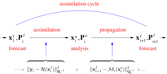
Figure 1.1: Data assimilation cycle of the Kalman filter.

There are a few things to be noted about the KF:

1. It follows from the Kalman filter (equations 1.4-1.7) that the state of the DA system (SDAS) $\mathbf{X}$ is carried by the estimated model state vector and model state error covariance:

   $$\mathbf{X}_{k}=\{\mathbf{x}_{k},\mathbf{P}_{k}\}.$$ (1.8)

2. The KF provides solution for the last analysis, corresponding to $\mathbf{x}_{k}^{a}$ in (1.1) (or, with a minor re-formulation, to the last forecast); finding the full (global in time) solution requires application of the Kalman smoother (KS). Both the KF and KS can be derived by decomposition of the positive (semi)definite quadratic function (1.2).

3. Because the SDAS represents a (part of a) solution of the global least squares problem, it does not depend on the order in which observations are assimilated or on their grouping.

4. Ditto, the SDAS does not depend on a linear non-singular transform of the model state in the sense that the forward and inverse transforms commute with the evolution of the DA system.

5. Solution (1.7, 1.6) can be used in a nonlinear case by approximating

   $$\mathbf{M}_{i}\leftarrow\nabla\mathcal{M}_{i}(\mathbf{x}_{i-1}^{a}),$$

   $$\mathbf{H}_{i}\leftarrow\nabla\mathcal{H}_{i}(\mathbf{x}_{i}^{f}),$$

   in which case it is called the extended Kalman filter (EKF).

1.2 EnKF

The standard form of the KF (1.7, 1.6) is not necessarily the most convenient or suitable one in practice. The corresponding algorithms can be prone to loosing the positive definiteness of the state error covariance $\mathbf{P}$ due to round-up errors; and more importantly, explicit use of $\mathbf{P}$ makes these algorithms non-scalable in regard to the model state dimension.

Both these immediate problems can be addressed with the ensemble Kalman filter, or the EnKF. In the EnKF the SDAS is carried by an ensemble of $m$ model states $\mathbf{E}$, which can be split into ensemble mean and ensemble anomalies:

$$\mathbf{X}=\{\mathbf{E}\}=\{\mathbf{x},\mathbf{A}\}.$$ (1.9)

It is related to the SDAS of the KF (1.8) as follows:

$$\mathbf{x}=\frac{1}{m}\mathbf{E}\,\mathbf{1},$$ (1.10a)

$$\mathbf{P}=\frac{1}{m-1}\mathbf{A}\mathbf{A}^{\tiny\mathrm{T}},$$ (1.10b)

$$\mathbf{A}\equiv\mathbf{E}-\mathbf{x}\mathbf{1}^{\tiny\mathrm{T}},$$ (1.10c)

where $\mathbf{1}$ is a vector with all elements equal to 1. The above means that the model state estimate is given by the ensemble mean, while the model state error covariance $\mathbf{P}$ is implicitly represented by the ensemble anomalies $\mathbf{A}$ via the factorisation (1.10b).

Representing the state error covariance via ensemble anomalies yields a number of numerical benefits. In large-scale geophysical systems the state size ($\sim 10^{5}-10^{9}$) makes it impossible to store and manipulate the state error covariance $\mathbf{P}$ directly. At the same time it is often/typically possible to represent essential variability via an ensemble of much smaller size ($\sim 10^{2}$) and manipulate $\mathbf{P}$ implicitly via operations with $\mathbf{A}$. Further, using $\mathbf{A}$ ensures positive semidefiniteness of $\mathbf{P}$.

Storing the SDAS via an ensemble of model states is the first essential feature of the EnKF. In theory, one could use it in an implementation of the KF along with explicitly calculated Jacobians $\mathbf{M}$ and $\mathbf{H}$ in equations (1.7) and (1.6). The EnKF makes a further step and uses the ensemble form of the SDAS for a derivative-less formulation of the KF. Moreover, it approximates derivatives using ensemble of finite spread that characterises the estimated uncertainty in the state:

$$\mathbf{E}\quad \leftarrow \quad\mathbf{x}\mathbf{1}^{\tiny\mathrm{T}}+\mathbf{A}\hskip 227.62204pt$$ (1.11a)

$$\mathcal{H}(\mathbf{x})\quad \to \quad\mathcal{H}(\mathbf{E})\,\mathbf{1}/m$$ (1.11b)

$$\mathbf{H}\mathbf{A}\quad \to \quad\mathcal{H}(\mathbf{E})\left(\mathbf{I}-\mathbf{1}\mathbf{1}^{\tiny\mathrm{T}}/m\right)$$ (1.11c)

$$\mathcal{M}(\mathbf{x})\quad \to \quad\mathcal{M}(\mathbf{E})\,\mathbf{1}/m$$ (1.11d)

$$\mathbf{M}\mathbf{A}\quad \to \quad\mathcal{M}(\mathbf{E})\left(\mathbf{I}-\mathbf{1}\mathbf{1}^{\tiny\mathrm{T}}/m\right)$$ (1.11e)

$$\mathbf{H}\mathbf{M}\mathbf{A} \to \quad\mathcal{H}\circ\mathcal{M}(\mathbf{E})\left(\mathbf{I}-\mathbf{1}\mathbf{1}^{\tiny\mathrm{T}}/m\right).$$ (1.11f)

This formulation is not the only one possible; one might also use the finite difference approximations:

$$\mathbf{E}\quad \leftarrow \quad\mathbf{x}\mathbf{1}^{\tiny\mathrm{T}}+\varepsilon\mathbf{A}\hskip 227.62204pt$$ (1.12a)

$$\mathbf{H}\mathbf{A}\quad \to \quad\mathcal{H}(\mathbf{E})\left(\mathbf{I}-\mathbf{1}\mathbf{1}^{\tiny\mathrm{T}}/m\right)/\varepsilon$$ (1.12b)

$$\mathbf{M}\mathbf{A}\quad \to \quad\mathcal{M}(\mathbf{E})\left(\mathbf{I}-\mathbf{1}\mathbf{1}^{\tiny\mathrm{T}}/m\right)/\varepsilon$$ (1.12c)

$$\mathbf{H}\mathbf{M}\mathbf{A}\quad \to \quad\mathcal{H}\circ\mathcal{M}(\mathbf{E})\left(\mathbf{I}-\mathbf{1}\mathbf{1}^{\tiny\mathrm{T}}/m\right)/\varepsilon.$$ (1.12d)

In this form the filter represents a derivative-less ensemble formulation of the EKF. In practice the difference between the EnKF formulation (1.11) and the EKF formulation (1.12) is that the latter is more sensitive to small-scale variability and therefore more prone to instability, similar to the difference in behaviour of the Newton and secant methods.

The forecast stage of the EnKF involves just propagating each ensemble member:

$$\mathbf{E}_{i}^{f}=\mathcal{M}_{i}(\mathbf{E}_{i-1}^{a}).$$ (1.13)

This is a remarkably simple equation compared to the KF forecast equations (1.7), even though the model error still needs to be accounted for in some way. Because propagation of each ensemble member is independent from the other members, the forecast stage in the EnKF is naturally parallelisable.

One way to handle model error in the EnKF is to include stochastic model error into the model operator in (1.13). (This would make it different to the model operator in the KF, which is deterministic.) Another option is to use the multiplicative inflation. The third option is to mimic the treatment of model error in the KF, although this would require the “rank reduction” (Verlaan and Heemink, 1997, eq. 28) to prevent increasing the ensemble size.

At the analysis stage one has to update the ensemble mean and ensemble anomalies to match (1.6). This involves handling ensemble as a whole, which is different to the forecast stage, when each ensemble member is propagated individually.

Note that factorisation (1.10b) is not unique: if $\mathbf{A}$ satisfies (1.10b), then $\tilde{\mathbf{A}}=\mathbf{A}\mathbf{U}$, where $\mathbf{U}$ is an arbitrary orthonormal matrix $\mathbf{U}\mathbf{U}^{\tiny\mathrm{T}}=\mathbf{I}$, also satisfies (1.10b). However, $\tilde{\mathbf{A}}$ should not only factorise $\mathbf{P}$, but also remain an ensemble anomalies matrix, $\tilde{\mathbf{A}}\mathbf{1}=\mathbf{0}$. This requires an additional constraint $\mathbf{U}\mathbf{1}=\mathbf{1}$. Summarising, if $\mathbf{E}=\mathbf{x}\mathbf{1}^{\tiny\mathrm{T}}+\mathbf{A}$ is an ensemble that satisfies (1.10), then ensemble

$$\tilde{\mathbf{E}}=\mathbf{x}\mathbf{1}^{\tiny\mathrm{T}}+\mathbf{A}\mathbf{U}^{p},\quad\mathbf{U}^{p}:\ \mathbf{U}^{p}(\mathbf{U}^{p})^{\tiny\mathrm{T}}=\mathbf{I},\ \mathbf{U}^{p}\mathbf{1}=\mathbf{1}$$ (1.14)

also satisfies (1.10). If $\mathbf{E}$ is full rank (i.e. $\mathrm{rank}(\mathbf{E})=\mathrm{min}(m,n)$, where $n$ is the state dimension), then each unique $\mathbf{U}^{p}$ generates a unique ensemble, and (1.14) describes all possible ensembles matching a given SDAS of the KF. Such transformation of the ensemble is called ensemble redrawing. In the linear case (i.e. for affine model and observation operators) redrawing of the ensemble in the EnKF does not affect evolution of the underlying KF; and conversely, in the nonlinear case the redrawing does indeed affect evolution of the underlying KF.

1.3 EnKF analysis

In this section we will give a brief overview of solutions for the EnKF analysis, and then describe the particular schemes used in EnKF-C.

1.3.1 Overview

In the “baseline” EnKF (full-rank ensemble, no localisation) the analysed SDAS matches that of the KF, although the algebraic side is indeed different. The update of the ensemble mean is generally straightforward, in accordance with that in the KF (1.6a). The details may depend on the chosen algorithm to achieve better numerical efficiency (see sec. 1.3.3).

The update of ensemble anomalies can be done either via a right-multiplied or left-multiplied (or post/pre-multiplied) transform of the ensemble anomalies:

$$\mathbf{A}^{a}=\mathbf{T}_{L}\,\mathbf{A}^{f},$$ (1.15)

or

$$\mathbf{A}^{a}=\mathbf{A}^{f}\,\mathbf{T}_{R}.$$ (1.16)

$\mathbf{T}_{L}$ and $\mathbf{T}_{R}$ are referred to hereafter as left-multiplied and right-multiplied ensemble transform matrices (ETMs), respectively. Note that to preserve the ensemble mean $\mathbf{T}_{R}$ has to satisfy $\mathbf{T}_{R}\mathbf{1}=\alpha\mathbf{1}$, where $\alpha$ is an arbitrary constant. It follows from (1.14) that if $\mathbf{T}_{R}$ is a particular solution for the right-multiplied ETM, then (for a full rank ensemble) any other solution can be written as

$$\tilde{\mathbf{T}}_{R}=\mathbf{T}_{R}\mathbf{U}^{p},\quad\mathbf{U}^{p}:\ \mathbf{U}^{p}(\mathbf{U}^{p})^{\tiny\mathrm{T}}=\mathbf{I},\ \mathbf{U}^{p}\mathbf{1}=\mathbf{1}.$$ (1.17)

(More generally, one could write $\tilde{\mathbf{T}}_{R}=\mathbf{T}_{R}(\mathbf{U}^{p}+\mathbf{1}\mathbf{a}^{\tiny\mathrm{T}})$, where $\mathbf{a}$ is an arbitrary vector, but this additional term does not change the ensemble.)

Similarly, the analysis increment can be represented as a linear combination of the forecast ensemble anomalies:

$$\mathbf{x}^{a}=\mathbf{x}^{f}+\mathbf{A}^{f}\mathbf{w}.$$ (1.18)

Equations (1.16) and (1.18) can be combined into a single transform of the ensemble:

$$\mathbf{E}^{a}=\mathbf{E}^{f}\mathbf{X}_{5},$$ (1.19)

$$\mathbf{X}_{5}=\frac{1}{m}\mathbf{1}\mathbf{1}^{\tiny\mathrm{T}}+\left(\mathbf{I}-\frac{1}{m}\mathbf{1}\mathbf{1}^{\tiny\mathrm{T}}\right)\left(\mathbf{w}\mathbf{1}^{\tiny\mathrm{T}}+\mathbf{T}_{R}\right)=\frac{1}{m}\mathbf{1}\mathbf{1}^{\tiny\mathrm{T}}+\mathbf{w}\mathbf{1}^{\tiny\mathrm{T}}+\left(\mathbf{I}-\frac{1}{m}\mathbf{1}\mathbf{1}^{\tiny\mathrm{T}}\right)\mathbf{T}_{R},$$ (1.20)

as $\mathbf{1}^{\tiny\mathrm{T}}\mathbf{w}=0$. When $\mathbf{T}_{R}:\ \mathbf{T}_{R}^{\tiny\mathrm{T}}=\mathbf{T}_{R},\ \mathbf{T}_{R}\mathbf{1}=\mathbf{1}$ (which is the case for e.g. the ETKF and DEnKF), $\mathbf{1}^{\tiny\mathrm{T}}\mathbf{T}_{R}=\mathbf{1}^{\tiny\mathrm{T}}$, and (1.20) simplifies to

$$\mathbf{X}_{5}=\mathbf{w}\mathbf{1}^{\tiny\mathrm{T}}+\mathbf{T}_{R}.$$ (1.21)

The designation $\mathbf{X}_{5}$ is used for historic reasons, following Evensen (2003).

1.3.2 Some schemes

As follows from the previous section, there are multiple solutions for the ETM that match the KF covariance update equation (1.6b); however the particular solutions may have different properties in practice due to the DAS nonlinearity, their algorithmic convenience, or their robustness in suboptimal conditions. This section provides some background for the schemes used in EnKF-C:

• ETKF;

• DEnKF.

ETKF

It is easy to show using the definition of $\mathbf{K}$ (1.6c) and matrix shift lemma (1.23) that

$$(\mathbf{I}-\mathbf{K}\mathbf{H})\,\mathbf{P}^{f}=(\mathbf{I}-\mathbf{K}\mathbf{H})^{1/2}\;\mathbf{P}^{f}\;(\mathbf{I}-\mathbf{K}\mathbf{H})^{{\mathrm{T}}/2},$$

which yields the following solution for the left-multiplied ETM:

$$\mathbf{T}_{L}=(\mathbf{I}-\mathbf{K}\mathbf{H})^{1/2}$$ (1.22)

(Sakov and Oke, 2008b), that is

$$\mathbf{A}^{a}=(\mathbf{I}-\mathbf{K}\mathbf{H})^{1/2}\mathbf{A}^{f}.$$ (1.22a)

Hereafter by $\mathbf{X}^{1/2}$ we denote the unique positive definite square root of a positive definite (generally, non-symmetric) matrix $\mathbf{X}$, defined as $\mathbf{X}^{1/2}=\mathbf{V}\mathbf{L}^{1/2}\mathbf{V}^{-1}$, where $\mathbf{X}=\mathbf{V}\mathbf{L}\mathbf{V}^{-1}$ is the eigenvalue decomposition of $\mathbf{X}$. By “matrix shift lemma” we refer to the following identity:

$$\mathcal{F}(\mathbf{A}\mathbf{B})\,\mathbf{A}=\mathbf{A}\,\mathcal{F}(\mathbf{B}\mathbf{A}),$$ (1.23)

where $\mathcal{F}$ is an arbitrary function expandable into Taylor series. Rewriting (1.22a) as

$$\mathbf{A}^{a}=\left[\mathbf{I}-\frac{1}{m-1}\mathbf{A}^{f}(\mathbf{H}\mathbf{A}^{f})^{\tiny\mathrm{T}}(\mathbf{H}\mathbf{P}^{f}\mathbf{H}^{\tiny\mathrm{T}}+\mathbf{R})^{-1}\mathbf{H}\right]^{1/2}\mathbf{A}^{f}$$

and using the matrix shift lemma, we obtain:

$$\mathbf{A}^{a}=\mathbf{A}^{f}\left[\mathbf{I}-\frac{1}{m-1}(\mathbf{H}\mathbf{A}^{f})^{\tiny\mathrm{T}}(\mathbf{H}\mathbf{P}^{f}\mathbf{H}^{\tiny\mathrm{T}}+\mathbf{R})^{-1}\mathbf{H}\mathbf{A}^{f}\right]^{1/2}$$

which yields the corresponding to (1.22) right-multiplied ETM:

$$\mathbf{T}_{R}=\left[\mathbf{I}-\frac{1}{m-1}(\mathbf{H}\mathbf{A}^{f})^{\tiny\mathrm{T}}(\mathbf{H}\mathbf{P}^{f}\mathbf{H}^{\tiny\mathrm{T}}+\mathbf{R})^{-1}\mathbf{H}\mathbf{A}^{f}\right]^{1/2}$$ (1.24)

(Evensen, 2004). Applying the matrix inversion lemma

$$(\mathbf{A}+\mathbf{U}\mathbf{L}\mathbf{V})^{-1}=\mathbf{A}^{-1}-\mathbf{A}^{-1}\mathbf{U}(\mathbf{L}^{-1}+\mathbf{V}\mathbf{A}^{-1}\mathbf{U})^{-1}\mathbf{V}\mathbf{A}^{-1},$$ (1.25)

(1.22) can be transformed to:

$$\mathbf{T}_{L}=(\mathbf{I}+\mathbf{P}^{f}\mathbf{H}^{\tiny\mathrm{T}}\mathbf{R}^{-1}\mathbf{H})^{-1/2}$$ (1.26)

(Sakov and Bertino, 2011); and applying the matrix shift lemma yields the corresponding right-multiplied ETM:

$$\mathbf{T}_{R}=\left[\mathbf{I}+\frac{1}{m-1}(\mathbf{H}\mathbf{A}^{f})^{\tiny\mathrm{T}}\mathbf{R}^{-1}\mathbf{H}\mathbf{A}^{f}\right]^{-1/2},$$ (1.27)

also known as the ensemble transform Kalman filter, or ETKF (Bishop et al., 2001).

Historic reference. Another (and probably the first) solution for $\mathbf{T}_{R}$ equivalent to (1.24) and (1.27) was found by Andrews (1968):

$$\mathbf{T}_{R}=\mathbf{I}-\frac{1}{m-1}(\mathbf{H}\mathbf{A}^{f})^{\tiny\mathrm{T}}\mathbf{M}^{-1/2}\left(\mathbf{M}^{1/2}+\mathbf{R}^{1/2}\right)^{-1}\mathbf{H}\mathbf{A}^{f},$$ (1.28)

where $\mathbf{M}\equiv\mathbf{H}\mathbf{P}^{f}\mathbf{H}^{\tiny\mathrm{T}}+\mathbf{R}$.

Equations (1.24, 1.27, 1.28) yield algebraically different expressions for the (unique) symmetric right-multiplied solution. Apart from being the only symmetric solution, it also represents the minimum distance solution for the ensemble anomalies: its ensemble of analysed anomalies is closer to the ensemble of forecast anomalies with the inverse forecast (or analysis) covariance as the metric than any other ensemble of analysed anomalies given by (1.17) (Ott et al., 2003, rev. 2005). This means that in the above sense the symmetric right-multiplied solution preserves the identities of ensemble members during analysis in the best possible way.

Note that while the left-multiplied solutions (1.22, 1.26) correspond to the symmetric right-multiplied solution, they are not symmetric.

In a typical DAS with a large scale model one can expect $m=100$, $p=10^{3}-10^{7}$, $n=10^{6}-10^{9}$; that is

$$m\ll p\ll n.$$ (1.29)

Therefore, considering the size of ETMs ($n\times n$ for left-multiplied ETMs and $m\times m$ for right-multiplied ETMs), only right-multiplied solutions are suitable for use with large scale models. The ETKF solution (1.27) represents the most popular option due to its simple form and numerical effectiveness: for a diagonal $\mathbf{R}$, it only requires to calculate inverse square root of a symmetric $m\times m$ matrix. Also, along with the left-multiplied solution (1.26), it generally has better numerical properties than solutions (1.22) and (1.24) due to the fact that the inverse square root in it is calculated from the sum of a positive definite and a positive semi-definite matrices.

DEnKF

Assuming that $\mathbf{K}\mathbf{H}$ is small in some sense, one can approximate solution (1.22) by expanding it into Taylor series about $\mathbf{I}$ and keeping the first two terms of the expansion:

$$\mathbf{T}_{L}=\mathbf{I}-\frac{1}{2}\mathbf{K}\mathbf{H}.$$ (1.30)

This approximation is known as the deterministic ensemble Kalman filter, or DEnKF (Sakov and Oke, 2008a). It has a simple interpretation of using half of the Kalman gain for updating the ensemble anomalies; but apart from that the DEnKF often represents a good practical choice due to its algorithmic convenience and good performance in suboptimal situations. The DEnKF is the default scheme in EnKF-C.

1.3.3 Some numerical considerations

Instead of using the forecast ensemble observation anomalies $\mathbf{H}\mathbf{A}^{f}$ and innovation $\mathbf{y}-\mathcal{H}(\mathbf{x}^{f})$ it is convenient to use their standardised versions:

$$\mathbf{s}=\mathbf{R}^{-1/2}\left[\mathbf{y}-\mathcal{H}(\mathbf{x}^{f})\right]/\sqrt{m-1},$$ (1.31)

$$\mathbf{S}=\mathbf{R}^{-1/2}\mathbf{H}\mathbf{A}^{f}/\sqrt{m-1}.$$ (1.32)

Then

$$\mathbf{w}=\mathbf{G}\mathbf{s};$$ (1.33)

for the ETKF

$$\mathbf{T}_{R}=(\mathbf{I}+\mathbf{S}^{\tiny\mathrm{T}}\mathbf{S})^{-1/2},$$ (1.34)

and for the DEnKF

$$\mathbf{T}_{R}=\mathbf{I}-\frac{1}{2}\mathbf{G}\mathbf{S},$$ (1.35)

where

$$\mathbf{G} \equiv(\mathbf{I}+\mathbf{S}^{\tiny\mathrm{T}}\mathbf{S})^{-1}\mathbf{S}^{\tiny\mathrm{T}},$$ (1.36)

$$=\mathbf{S}^{\tiny\mathrm{T}}(\mathbf{I}+\mathbf{S}\mathbf{S}^{\tiny\mathrm{T}})^{-1}.$$ (1.37)

Here (1.36) involves inversion of an $m\times m$ matrix, while (1.37) involves inversion of a $p\times p$ matrix. Therefore, in the DEnKF it is possible to calculate $\mathbf{w}$ and $\mathbf{T}$ using a single inversion of either a $p\times p$ or $m\times m$ matrix, depending on the relation between the number of observations and the ensemble size. In contrast, the ETKF (1.34) requires calculation of the inverse square root of an $m\times m$ matrix. Then, one can use expression (1.36) for $\mathbf{G}$ and calculate both inversion in it and inverse square root in (1.34) from the same singular value decomposition (SVD). This makes the DEnKF somewhat more numerically effective because, firstly, one can exploit situations when $p<m$ to invert a matrix of lower dimension and, secondly, it requires only matrix inversion, which can be done via Cholesky decomposition instead of SVD.

1.4 Localisation

Localisation is a necessary attribute of the EnKF systems with large-scale models, aimed at overcoming the rank deficiency of the ensemble. It can also be seen as aimed at reducing spurious long range correlations occurring due to the finite size of the ensemble; or at limiting the impact of distant observations because of the unreliability of the corresponding covariances.

There are two common localisation methods for the EnKF – covariance localisation (CL, Hamill and Whitaker, 2001; Houtekamer and Mitchell, 2001), also known as covariance filtering, and local analysis (LA, Evensen, 2003; Ott et al., 2003, rev. 2005). Although CL may have advantages in certain situations (non-local observations, “strong” assimilation), in practice the two methods produce similar results (Sakov and Bertino, 2011). For algorithmic reasons EnKF-C uses LA.

Instead of calculating the global ensemble transform $\mathbf{X}_{5}$, LA involves calculating local ensemble transforms $\accentset{i}{\mathbf{X}}_{5}$ for each element $i$ of the state vector. This is done using local normalised ensemble observation anomalies $\accentset{i}{\mathbf{S}}$ and local normalised innovation $\accentset{i}{\mathbf{s}}$, obtained by tapering global $\mathbf{S}$ and $\mathbf{s}$:

$$\accentset{i}{\mathbf{s}}\equiv\mathbf{s}\circ\accentset{i}{\mathbf{f}},$$ (1.38a)

$$\accentset{i}{\mathbf{S}}\equiv\mathbf{S}\circ(\accentset{i}{\mathbf{f}}\,\mathbf{1}^{\tiny\mathrm{T}}),$$ (1.38b)

where $\accentset{i}{\mathbf{f}}$ is the vector of taper coefficients for element $i$, and $\mathbf{A}\circ\mathbf{B}$ denotes by-element, or Hadamard, or Schur product of matrices $\mathbf{A}$ and $\mathbf{B}$. We consider non-adaptive localisation only, when the taper coefficient is a function of locations of the state element $i$ (denoted as $\accentset{i}{\mathbf{r}}$) and observation $o$ (denoted as $\accentset{\{o\}}{\mathbf{r}}$): $\accentset{i}{\mathbf{f}}_{o}=g(\accentset{i}{\mathbf{r}},\accentset{\{o\}}{\mathbf{r}})$, where $g$ is the taper function. In layered geophysical models $g$ is often assumed to depend only on horizontal distance between these locations:

$$\accentset{i}{\mathbf{f}}_{o}=g(|\accentset{i}{\boldsymbol{\rho}}-\accentset{\{o\}}{\boldsymbol{\rho}}|),$$ (1.39)

or on combination of horizontal and vertical distances, e.g.: $\accentset{i}{f}_{o}=g_{xy}(|\accentset{i}{\boldsymbol{\rho}}-\accentset{\{o\}}{\boldsymbol{\rho}}|)g_{z}(|\accentset{i}{z}-\accentset{\{o\}}{z}|)$, where $\mathbf{r}=(\boldsymbol{\rho},z)$, and $\boldsymbol{\rho}=(x,y)$. In the case (1.39) for a given set of observations the local ensemble transform $\accentset{i}{\mathbf{X}}_{5}$ depends only on horizontal grid coordinates of the state element $\mathbf{x}_{i}$ and can be used for updating all state elements with the same horizontal grid coordinates. This is currently the only option in EnKF-C.

Smooth taper functions have advantage over non-smooth functions (such as the boxcar, or step function) because they maintain the spatial continuity of the analysis. EnKF-C uses the popular polynomial taper function by Gaspari and Cohn (1999), which has a number of nice properties.

1.5 Asynchronous DA

Observations assimilated at each cycle in the KF are assumed to be made simultaneously at the time of assimilation. In such cases observations and DA method are referred to as synchronous. In reality, observations assimilated at a given cycle are made over some period of time called “data assimilation window” (DAW). If the DA method accounts for the time of observations, observations and DA method are referred to as asynchronous.

The EnKF can be naturally extended for asynchronous DA. Let us consider the minimisation problem (1.1, 1.2) in the case of perfect model $\mathbf{Q}=0$. It becomes

$${\mathbf{x}_{1}^{a}}=\arg\min\;J(\mathbf{x}_{1}),$$ (1.40)

$$J(\mathbf{x}_{1})=\|\mathbf{x}_{1}-\mathbf{x}_{1}^{f}\|^{2}_{(\mathbf{P}_{1}^{f})^{-1}}+\sum_{i=1}^{k}\|\mathbf{y}_{i}-\mathcal{H}_{i}(\mathbf{x}_{i})\|^{2}_{(\mathbf{R}_{i})^{-1}},$$ (1.41)

$$\mathbf{x}_{i+1}=\mathcal{M}(\mathbf{x}_{i}),\quad i=1,\dots,k-1.$$ (1.42)

Compared to the original problem, the dimensionality of the solution is much reduced due to relations (1.42), which mean that the model state at any time can be found by propagating the initial state: $\mathbf{x}_{2}=\mathcal{M}_{2}(\mathbf{x}_{1}),\ \mathbf{x}_{3}=\mathcal{M}_{3}\circ\mathcal{M}_{2}(\mathbf{x}_{1}),\dots$. The cost function (1.41) can then be written as

$$J(\mathbf{x}_{1})=\|\mathbf{x}_{1}-\mathbf{x}_{1}^{f}\|^{2}_{(\mathbf{P}^{f})^{-1}}+\|\mathbf{y}-\mathcal{H}\circ\mathcal{M}(\mathbf{x}_{1})\|^{2}_{\mathbf{R}^{-1}},$$ (1.43)

where observations $\mathbf{y}$ represent the augmented observation vector: $\mathbf{y}=[\mathbf{y}_{1}^{\tiny\mathrm{T}},\dots,\mathbf{y}_{k}^{\tiny\mathrm{T}}]^{\tiny\mathrm{T}}$, $\mathbf{R}$ is the corresponding observation error covariance, and forward operator $\mathcal{H}\circ\mathcal{M}(\mathbf{x}_{1})$ relates the initial state $\mathbf{x}_{1}$ to observations.

Note that usually only $\mathcal{H}$ is a function that depends on assimilated observations; now by introducing $\mathcal{H}\circ\mathcal{M}(\mathbf{x})=\mathcal{H}[\mathcal{M}(\mathbf{x})]$ we have to assume that $\mathcal{M}$ also depends on observations, propagating the initial state to the time of each observation. It is also possible to interpret $\mathcal{M}(\mathbf{x}$) as the trajectory starting from $\mathbf{x}$, while $\mathcal{H}$ maps it to observations.

Apart from the operator $\mathcal{H}\circ\mathcal{M}$, the cost function (1.43) has the same form as that for a single DA cycle with synchronous observations. Consequently, in the linear case (1.3) one can use solutions for $\mathbf{w}$ and $\mathbf{T}$ from section 1.3.3, subject to extending definitions of $\mathbf{s}$ (1.31) and $\mathbf{S}$ (1.32) as follows:

$$\mathbf{s}=\mathbf{R}^{-1/2}\left[\mathbf{y}-\mathcal{H}\circ\mathcal{M}(\mathbf{x}_{1}^{f})\right]/\sqrt{m-1},$$ (1.44)

$$\mathbf{S}=\mathbf{R}^{-1/2}\,\mathbf{H}\circ\mathbf{M}\,\mathbf{A}_{1}^{f}/\sqrt{m-1},$$ (1.45)

where $\mathbf{H}\circ\mathbf{M}$ is the tangent linear operator of $\mathcal{H}\circ\mathcal{M}$ about $\mathbf{x}_{1}^{f}$. This means that to account for the time of observations in the EnKF one simply needs calculate innovation and forecast ensemble observation anomalies using ensemble at the time of each observation. There are no specific restrictions on $\mathbf{R}$, so that in theory observation errors can be correlated in time.

The minimisation problem (1.40),(1.43) implies assimilation time $t=t_{1}$; however, in the linear case the standardised innovation and ensemble observation anomalies in form (1.44,1.45) represent objects invariant to assimilation time: the reference to $\mathbf{x}_{1}$ is only needed to define forward operator $\mathcal{H}\circ\mathcal{M}$. Consequently, the ensemble transform $\mathbf{X}_{5}$ calculated from $\mathbf{s}$ and $\mathbf{S}$ can be applied to ensemble at any particular time to yield (the same) analysed trajectories for the ensemble members: $\mathcal{M}(\mathbf{E})\,\mathbf{X}_{5}=\mathcal{M}(\mathbf{E}\,\mathbf{X}_{5})$. This time invariance of ensemble transforms can be used to update ensemble back in time using observations from future cycles without the need in backward model (Evensen and van Leeuwen 2000, sec. 6, Evensen 2003, app. D).

Note. The background term $\|\mathbf{x}_{1}-\mathbf{x}_{1}^{f}\|^{2}_{(\mathbf{P}^{f})^{-1}}$ in (1.43) can be seen as accumulating the previous history of the system rather than characterising the initial uncertainty in the global problem. In this case it is natural to anchor it to the previous analysis:

$$J(\mathbf{x})=\|\mathbf{x}-\mathbf{x}^{f}\|^{2}_{(\mathbf{P}^{f})^{-1}}+\|\mathbf{y}-\mathcal{H}\circ\mathcal{M}(\mathbf{x})\|^{2}_{\mathbf{R}^{-1}}.$$ (1.46)

Here $\mathbf{x}^{f}$ is the forecast state at the start of the cycle obtained from the previous analysis, and $\mathbf{P}^{f}$ is the corresponding state error covariance. Minimising $J$ yields the analysed initial model state $\mathbf{x}^{a}$, which in turn yields the analysed trajectory. The analysed state error covariance is defined so that the analysed background term absorbs the observation term:

$$\mathbf{x}^{a},\mathbf{P}^{a}:\ J(\mathbf{x})=\|\mathbf{x}-\mathbf{x}^{a}\|^{2}_{(\mathbf{P}^{a})^{-1}}+\mathrm{Const}.$$

This framework is a natural extension of the problem (1.1) in the linear, perfect-model case to continuous time; and is convenient for iterative minimisation.

1.6 EnOI

The EnOI, or ensemble optimal interpolation (Evensen, 2003), can be defined as the EnKF with a static or, more generally, pre-defined, ensemble anomalies. It can be summarised as follows:

$$\mathbf{x}^{b}_{i}=\mathcal{M}_{i}(\mathbf{x}^{a}_{i-1}),$$ (1.47)

$$\mathbf{x}^{a}_{i}=\mathbf{x}^{b}_{i}+\mathbf{A}^{b}\,\mathbf{w}_{i},$$ (1.48)

where $\mathbf{x}^{b}$ is the forecast model state estimate referred to as background, and $\mathbf{A}^{b}$ is an ensemble of static, or background, anomalies; the corresponding state error covariance $\mathbf{P}^{b}$ is also often referred to as the background covariance.

The main incentive for using the EnOI is its low computational cost due to the integration of only one instance of the model. Despite of the similarity with the EnKF, the EnOI is a rather different concept, as there is no global in time cost function associated with it. Conceptually the EnOI is closer to 3D-Var, as both methods use static (anisotropic, multivariate) covariance. It is an improvement on the optimal interpolation, which typically uses isotropic, homogeneous and univariate covariance.

In contrast to the EnKF, due to the use of a static ensemble the EnOI avoids potential problems related to the ensemble spread; but at the same time it does critically depend on the ensemble, while the EnKF with a stochastic model typically “forgets” the initial ensemble over time.

The EnOI can account for the time of observations by calculating innovation using forecast at observation time, as in (1.44). This approach is commonly known as “first guess at appropriate time”, or FGAT.

1.7 EnOI/EnKF hybrid

By EnOI/EnKF hybrid we understand formulation in which forecast state error covariance is equal to the sum of “dynamic” covariance carried by the EnKF ensemble, and “static” covariance carried by a pre-defined ensemble of anomalies:

$$\mathbf{P}^{f}=\mathbf{P}^{\textnormal{dyn}}+\gamma\mathbf{P}^{\textnormal{stat}},$$ (1.49)

where

$$\mathbf{P}^{\textnormal{dyn}}=\frac{1}{m_{\textnormal{dyn}}-1}\mathbf{A}^{\textnormal{dyn}}(\mathbf{A}^{\textnormal{dyn}})^{\tiny\mathrm{T}},$$

$$\mathbf{P}^{\textnormal{stat}}=\frac{1}{m_{\textnormal{stat}}-1}\mathbf{A}^{\textnormal{stat}}(\mathbf{A}^{\textnormal{stat}})^{\tiny\mathrm{T}},$$

where $\mathbf{A}^{\textnormal{dyn}}$ is the ensemble of dynamic anomalies of size $m_{\textnormal{dyn}}$, and $\mathbf{A}^{\textnormal{stat}}$ is the ensemble of static anomalies of size $m_{\textnormal{stat}}$. The added static covariance can be assumed to represent the model error covariance (matrices $\mathbf{Q}_{i}$ in (1.2) and $\mathbf{Q}_{k+1}$ in (1.7b)).

The forecast covariance $\mathbf{P}^{f}$ is then carried by the combined ensemble $\mathbf{A}^{f}$,

$$\mathbf{A}^{f}=\left[\left(\frac{m-1}{m_{\textnormal{dyn}}-1}\right)^{1/2}\mathbf{A}^{\textnormal{dyn}},\left(\gamma\frac{m-1}{m_{\textnormal{stat}}-1}\right)^{1/2}\mathbf{A}^{\textnormal{stat}}\right],$$ (1.50)

where $m=m_{\textnormal{dyn}}+m_{\textnormal{stat}}$, so that

$$\mathbf{P}^{f}=\frac{1}{m-1}\mathbf{A}^{f}(\mathbf{A}^{f})^{\tiny\mathrm{T}}.$$

The combined forecast ensemble anomalies (1.50) have larger ensemble size than that of the dynamic ensemble; hence there arises a problem of ensemble reduction to obtain the analysed dynamic ensemble of size $m_{\textnormal{dyn}}$. There are a number of approaches to this problem. Perhaps the easiest one to implement is to use members of the analysed ensemble corresponding to the members of the dynamic forecast ensemble:

$$(\mathbf{E}^{\textnormal{dyn}})^{a}=\mathbf{E}^{f}\mathbf{X}_{5}(1:m,1:m_{\textnormal{dyn}}).$$

The forecast ensemble $\mathbf{E}^{f}$ is built from the combined forecast ensemble anomalies (1.50):

$$\mathbf{E}^{f}=\mathbf{x}^{f}\mathbf{1}^{\tiny\mathrm{T}}+\mathbf{A}^{f},$$ (1.51)

where the forecast state $\mathbf{x}^{f}$ is assumed to be equal to the mean of the dynamic ensemble only:

$$\mathbf{x}^{f}\equiv\frac{1}{m_{\textnormal{dyn}}}\mathbf{E}^{\textnormal{dyn}}.$$ (1.52)

Finally, note that in absence of observations $\mathbf{X}_{5}=\mathbf{I}$, $(\mathbf{E}^{\textnormal{dyn}})^{a}=\mathbf{E}^{f}(:,1:m_{\textnormal{dyn}})$, and according to (1.50)

$$(\mathbf{A}^{\textnormal{dyn}})^{a}=\left(\frac{m-1}{m_{\textnormal{dyn}}-1}\right)^{1/2}\mathbf{A}^{\textnormal{dyn}},$$

while for correct cycling of the system one needs $(\mathbf{A}^{\textnormal{dyn}})^{a}=\mathbf{A}^{\textnormal{dyn}}$. Therefore, it is necessary to scale $(\mathbf{A}^{\textnormal{dyn}})^{a}$ as follows:

$$(\mathbf{E}^{\textnormal{dyn}})^{a}=(\mathbf{x}^{f}+\mathbf{A}^{f}\mathbf{w})\mathbf{1}^{\tiny\mathrm{T}}+\left(\frac{m_{\textnormal{dyn}}-1}{m-1}\right)^{1/2}\mathbf{A}^{f}\mathbf{T}(1:m,1:m_{\textnormal{dyn}}).$$ (1.53)

This is the approach used in EnKF-C.

Chapter 2 EnKF-C

2.1 Design considerations

EnKF-C is designed to use horizontal localisation only. While some may argue that using vertical localisation might help to decrease the ensemble size, we believe that, for example, in the ocean the vertical structure is too complicated and non-uniform to allow simple and robust solutions in this regard. Generally, dynamical processes include a variety of barotropic and baroclinic components, and introducing vertical localisation in one form or another can be detrimental for the model’s balances. On the other hand, with an ensemble size of about 100, normally one can ignore the problem of spurious vertical correlations and leave the system to deal with the vertical covariances on its own.

With the system using horizontal localisation only, the model state effectively becomes a collection of independent horizontal fields updated based on their correlations with local ensemble observations. The assimilation is conducted by calculating a common horizontal array of local ensemble transforms and applying them to each horizontal field of the model. The local transforms are independent of each other and can be calculated in parallel, as well as the updates of the ensembles of horizontal model fields.

2.2 The workflow

EnKF-C conducts data assimilation in three stages: PREP, CALC and UPDATE.

PREP preprocesses observations so that they are ready for DA. It has the following stages:

• read original observations and convert them into a vector of structure observation;

• collate them into superobservations;

• write superobservations to observations.nc.

PREP does not need to access the model state; it only needs to access the model grid. (Note that for some types of vertical coordinates the vertical model grid depends on the state.)

CALC calculates ensemble transforms for updating the forecast ensemble of model states (EnKF) or the background model state (EnOI) in the following steps:

• read superobservations from observations.nc;

• calculate ensemble of forecast observations $\mathbf{H}\mathbf{E}^{f}$ (EnKF) or ensemble of background observation anomalies $\mathbf{H}\mathbf{A}^{f}$ and background observations $\mathbf{H}\mathbf{x}^{f}$ (EnOI);

• for nodes with specified stride on each horizontal grid get local observations and calculate local ensemble transforms $\mathbf{X}_{5}$ (EnKF) or local background update coefficients $\mathbf{w}$ (EnOI);

• save these transforms to transforms.nc (or transforms.nc-0, transforms.nc-1, … in multi-grid case);

• calculate and report forecast and analysis innovation statistics;

• calculate observation impact metrics DFS and SRF (sec. 2.7.6) and save them to enkf_diag.nc;

• at specified horizontal locations save the model state ensemble, observations, transforms/weights, and DA settings to pointlog files (sec. 2.11).

Apart from this main mode of operation, CALC can also be used for calculating the forecast innovations, or operate in the single observation experiment mode.

UPDATE updates the ensemble (EnKF) or the background (EnOI) using the transforms calculated by CALC, along with a number of specified diagnostics, such as the ensemble spread, inflation, or vertical correlations of subsurface fields with the surface field.

The principle diagram of EnKF-C workflow is shown in Fig. 2.1.

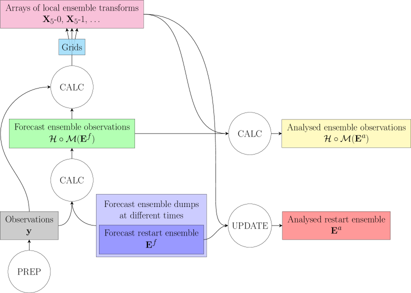
Figure 2.1: The principle diagram of EnKF-C workflow.

2.3 Starting up: example 1

It may be a good idea to start getting familiar with the system by running the example in examples/1. The example has been put up based on runs of the regional EnKF and EnOI reanalysis systems for Tasman Sea developed by Bureau of Meteorology. It allows one to conduct a single assimilation for 23 December 2007 (day 6565 since 1 January 1990) with either EnKF or EnOI. To reduce the size of the system, the model state has been stripped down to two vertical levels and $100\times 100$ horizontal grid. Due to its size (almost 80 MB) the data for this example is available for download separately from the EnKF-C code – see examples/1/README for details.

2.4 Parameter files

EnKF-C requires 5 parameter files to run (fig. 2.2):

• main parameter file;

• model parameter file;

• grid parameter file;

• observation types parameter file;

• and observation data parameter file.

Examples of these parameter files can be found in examples/1. Running EnKF-C binaries with --describe-prm-format in the command line provides information on the parameter file formats.

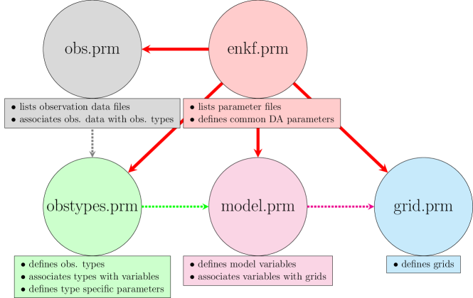
Figure 2.2: Parameter files in EnKF-C.

2.4.1 Main parameter file

The main parameter file specifies the main parameters of DA and 4 other parameter files. Its format is described by running enkf_prep, enkf_calc or enkf_update with option --describe-prm-format:

     >./bin/enkf_prep --describe-prm-format      Main parameter file format:        MODE            = { ENKF | ENOI | HYBRID }      MODEL           = <model prm file>    [ SCHEME          = { DENKF* | ETKF } ]                    (MODE = ENKF or HYBRID)    [ ALPHA           = <alpha> ]                              (1*) (MODE = ENKF or HYBRID)      GAMMA           = <gamma>                                (MODE = HYBRID)      GRID            = <grid prm file>      OBSTYPES        = <obs. types prm file>      OBS             = <obs. data prm file>      DATE            = <day of analysis>    [ WINDOWMIN       = <start of obs window in days from analysis> ] (-inf*)    [ WINDOWMAX       = <end of obs window in days from analysis> ]   (+inf*)      ENSDIR          = <ensemble directory>                   (except MODE = ENOI and                                                               --forecast-stats-only)    [ ENSDIR_STATIC   = <static ensemble directory> ]          (MODE = HYBRID)    [ ENSSIZE         = <ensemble size> ]                      (<full>*)    [ ENSSIZE_DYNAMIC = <size of dynamic ensemble> ]           (<full>*) (MODE = HYBRID)    [ ENSSIZE_STATIC  = <size of static ensemble> ]            (<full>*) (MODE = HYBRID)      BGDIR           = <background directory>                 (MODE = ENOI)    [ KFACTOR         = <kfactor> ]                            (NaN*)    [ RFACTOR         = <rfactor> ]                            (1*)      ...      LOCRAD          = <loc. radius in km> ...      LOCWEIGHT       = <loc. weight> ...                      (# LOCRAD > 1)    [ NLOBSMAX        = <max. number of local obs. of each type> ]    [ STRIDE          = <stride for ensemble transforms> ]     (1*)    [ SOBSTRIDE       = <stride for superobing> ]              (1*)    [ FIELDBUFFERSIZE = <fieldbuffersize> ]                    (1*)    [ INFLATION       = <inflation> [ <VALUE>* | PLAIN ]       (1*)      ...    [ REGION          = <name> <lon1> <lon2> <lat1> <lat2>      ...    [ POINTLOG        <lon> <lat> [grid name]]      ...    [ EXITACTION      = { BACKTRACE* | SEGFAULT } ]    [ BADBATCHES      = <obstype> <max. bias> <max. mad> <min # obs.> ]    [ NCFORMAT        = { CLASSIC | 64BIT | NETCDF4 } ]        (64BIT*)    [ NCCOMPRESSION   = <compression level> ]                  (0*)      ...      Notes:      1. { ... | ... | ... } denotes the list of possible choices      2. [ ... ] denotes an optional input      3. ( ... ) is a note      4. * denotes the default value      5. < ... > denotes a description of an entry      6. ... denotes repeating the previous item an arbitrary number of times     

Global analysis

It is possible to conduct global analysis by setting LOCRAD and STRIDE to large numbers. This is demonstrated by target “global” in example 1.

2.4.2 Model parameter file

The model parameter file mainly describes the composition of the state vector by listing the model variables and specifying the associated grids.

     >./bin/enkf_prep --describe-prm-format model      Model parameter file format:        NAME      = <name>      VAR       = <name>    [ GRID      = <name> ]                    (# grids > 1)    [ INFLATION = <value> [<value> | PLAIN] ]    [ APPLYLOG  = <YES | NO*> ]    [ RANDOMISE <deflation> <sigma> ]      [ <more of the above blocks> ]     

Each model variable is described in a block started by the entry for the variable name. The inflation parameters for a variable, if specified, override the common values set in the main parameter file (sec. 2.8.1). The option APPLYLOG makes it possible to conduct assimilation in log space (sec. 2.14), and RANDOMISE – to specify a “forgetting” model for the variable (sec. 2.13).

EnKF-C permits using multiple model grids. In this case each model variable must be associated with one of the grids defined in the grid parameter file. See examples/4 for an example.

2.4.3 Grid parameter file

Grid parameter file describes grids used for model variables. Each grid is described in a section started by the grid name entry and contains the grid name, grid data file, and names of the dimensions and coordinates in the grid data file. It also contains variable names for the depth and for number of layers in a vertical column (z grids) or land mask (sigma grids):

     >./bin/enkf_prep --describe-prm-format grid      Grid parameter file format:        NAME             = <name> [ PREP | CALC ]    [ DOMAIN           = <domain name> ]      DATA             = <data file name>      (either)        XVARNAME       = <X variable name>        YVARNAME       = <Y variable name>      (or)        HGRIDFROM      = <grid name>      (end either)      VTYPE            = { z | sigma | hybrid | none }    [ VDIR             = { fromsurf* | tosurf } ]      (if vtype = z)        ZVARNAME       = <Z variable name>      [ ZCVARNAME      = <ZC variable name> ]      [ NUMLEVELSVARNAME = <# of levels variable name> ]      [ DEPTHVARNAME   = <depth variable name> ]      (else if vtype = sigma)        CVARNAME       = <Cs_rho variable name>      [ CCVARNAME      = <Cs_w variable name> ]      [ SVARNAME       = <s_rho variable name> ]            (uniform*)      [ SCVARNAME      = <s_w variable name> ]              (uniform*)      [ HCVARNAME      = <hc variable name> ]               (0.0*)      [ DEPTHVARNAME   = <depth variable name> ]      [ MASKVARNAME    = <land mask variable name> ]      (else if vtype = hybrid)        AVARNAME       = <A variable name>        BVARNAME       = <B variable name>      [ ACVARNAME      = <AC variable name> ]      [ BCVARNAME      = <BC variable name> ]        P1VARNAME      = <P1 variable name>        P2VARNAME      = <P2 variable name>      [ MASKVARNAME    = <land mask variable name> ]      (end if)    [ STRIDE           = <stride for ensemble transforms> ] (1*)    [ SOBSTRIDE        = <stride for superobing> ]          (1*)    [ ZSTATINTS        = [<z1> <z2>] ... ]      [ <more of the above blocks> ]     

The code is supposed to automatically identify the type of horizontal grid used, while the type of the vertical grid has to be specified explicitly. If some grid (say, grid A) has the same horizontal grid as other grid (grid B), the code can be notified of this by entering name of grid A in the field HGRIDFROM for grid B (or vice versa). This saves memory, grid initialisation time, and uses transforms calculated for grid A for all variables defined on grid B.

Horizontal grids

At the moment, EnKF-C supports 3 main types of horizontal grids:

• equidistant rectangular grids aligned with physical coordinates;

• non-equidistant rectangular grids aligned with physical coordinates;

• quadrilateral grids.

The grid is assumed to be rectangular if grid node coordinates depend on one dimension, and quadrilateral (curvilinear) if they depend on two dimensions. For rectangular grids the code tries to determine and handle periodicity in X direction.

Note that the code does not detect and therefore can not take advantage of periodic curvilinear grids; because of that, it does not map (skips) observations in cells connecting the grid edges.

Vertical grids

The vertical coordinates are used for mapping the depth/height (pressure) of non-surface observations to fractional layer index. The observation depth or height are assumed to be positive.

The type of the vertical grid is defined by entry VTYPE in the grid parameter file. EnKF-C supports 3 types of vertical grids: $Z$ (“z”); $\sigma$ (“sigma”); and hybrid $\sigma$-$p$ ($\sigma$ - pressure, “hybrid”). It is also possible to define a purely horizontal (two-dimensional) grid by defining its vertical type as “none”.

For $Z$ grids one needs to define vertical coordinates of layer centres (entry ZVARNAME) and (optionally) the coordinates of layer corners (ZCVARNAME). If coordinates of layer corners are not specified they are built by the code assuming that the surface layer starts at $z=0$.

For $\sigma$ grids the code implements the “new” vertical coordinate formulation from ROMS as described in https://www.myroms.org/wiki/Vertical_S-coordinate, Eq. 2 and elaborated by Shchepetkin in https://www.myroms.org/forum/viewtopic.php?f=20&t=2189. This formulation reduces to the “standard” $\sigma$ grid if the entry HCVARNAME is not specified or if the corresponding variable in the grid file is set to zero. Similarly to $Z$ grid, one needs to define the vertical coordinates of layer centres (entry CSRVARNAME) and (optionally) the coordinates of layer corners (entry CSWVARNAME). From version 1.81.0 one can also specify variables for layer coordinates (which is used to be “plain” sigma, that is uniform) via entries SVARNAME and SCVARNAME.

The hybrid $\sigma$-$p$ grids are implemented as described in https://journals.ametsoc.org/doi/pdf/10.1175/2008MWR2537.1. One needs to specify the $A$ (AVARNAME) and $B$ (BVARNAME) arrays for layer centres as well as the top and surface pressure (P1VARNAME and P2VARNAME). One can also specify optional $A$ and $B$ arrays for layer corners (ACVARNAME, BCVARNAME). The entry DEPTHVARNAME needs only to be specified for variables with non-surface observations.

By default, the code assumes that the surface is at layer 0. If this is not the case, one needs to describe it explicitly by the entry VDIR = TOSURF; otherwise the surface ensemble or background observations will not be calculated correctly.

2.4.4 Observation types parameter file

Observation types are the interface that connects model and observations. They are specified in a separate parameter file. Each observation type is described in a separate section identified by the entry NAME. Apart from the type name, the section must contain the tag for the associated model variable and the tag for the associated observation operator. The optional parameters include the R-factor and localisation radius for the type (sec. 2.10), the allowed range, and spatial limits for the corresponding observations.

     >./bin/enkf_prep --describe-prm-format obstypes      Observation types parameter file format:        NAME        = <name>    [ DOMAINS     = <domain name> ... ]      ISSURFACE   = {0 | 1}    [ STATSONLY   = {0* | 1} ]      VAR         = <model variable name> ...    [ ALIAS       = <variable name used in file names> ]   (VAR*)    [ OFFSET      = <file name> <variable name> ]          (none*)    [ MLD_VARNAME = <model varname> ]                      (none*)    [ MLD_THRESH  = <threshold> ]                          (NaN*)    [ HFUNCTION   = <H function name> ]                    (standard*)    [ ASYNC       = <time interval> [c*|e [time varname]]] (0*)    [ LOCRAD      = <loc. radius in km> ... ]    [ LOCWEIGHT   = <loc. weight> ... ]                    (# LOCRAD > 1)    [ RFACTOR     = <rfactor> ]                            (1*)    [ NLOBSMAX    = <max. allowed number of local obs.> ]  (inf*)    [ ERROR_STD_MIN = <min. allowed superob error> ]       (0*)    [ SOBSTRIDE   = <stride for superobing> ]              (1*)    [ PERMIT_LOCATION_BASED_THINNING = <yes | no> ]        (yes*)    [ MINVALUE    = <minimal allowed value> ]              (-inf*)    [ MAXVALUE    = <maximal allowed value> ]              (+inf*)    [ XMIN        = <minimal allowed X coordinate> ]       (-inf*)    [ XMAX        = <maximal allowed X coordinate> ]       (+inf*)    [ YMIN        = <minimal allowed Y coordinate> ]       (-inf*)    [ YMAX        = <maximal allowed Y coordinate> ]       (+inf*)    [ ZMIN        = <minimal allowed Z coordinate> ]       (-inf*)    [ ZMAX        = <maximal allowed Z coordinate> ]       (+inf*)    [ WINDOWMIN   = <start of obs window in days from analysis> ] (-inf*)    [ WINDOWMAX   = <end of obs window in days from analysis> ]   (+inf*)      [ <more of the above blocks> ]     

The tags for available observation operators are listed in array allhentries in file calc/allhs.c.

The OFFSET entry may be used for adding the known model bias to observations, for example, to specify the mean dynamic topography (MDT) when assimilating sea level anomaly (SLA) observations. The dimension of the offset should match that of the corresponding model variable, except that it is possible to define (1D) layer-wise offsets for 3D model variables.

The localisation radius for an observation type, if specified, overrides the common value from the main parameter file. The R-factors for each observation type are obtained by multiplying the common value by the observation type value. (More on localisation radius and R-factor in sec. 2.10.)

The entries MLD_VARNAME and MLD_THRESH are used to calculate the model mixed layer depth for projecting the surface bias.

WINDOWMIN and WINDOWMAX define the allowed temporal interval for this observation type relatively to the analysis day and override the corresponding common settings in the main parameter file.

The use of ALIAS is described in sec. 2.5.

2.4.5 Observation data parameter file

Observation data parameter file specifies observations to be assimilated. EnKF-C has a simple policy in this regard: if a data file is listed in the observation data parameter file, then observations from this file are assimilated. This allows one using custom observation windows for particular observation types, instruments etc., specifying details on the script level during the parameter file generation.

In practice some of observations specified in the observation data parameter file can be outside the observation time window for the cycle. In this case the exact boundaries of the observation window can be specified by entries WINDOWMIN and WINDOWMAX in the main parameter file or (for specific observation types) observation types parameter file; observations with time outside interval [DATE-WINDOWMIN, DATE+WINDOWMAX) will be discarded.

The observation parameter file contains an arbitrary number of sections identified by entries PRODUCT. Each section specifies the observation type, input files, reader and, possibly, observation error:

     ./bin/enkf_prep --describe-prm-format obsdata      Observation data parameter file format:        PRODUCT   = <product>      READER    = <reader>    [ PARAMETER <name> = <value> ]      ...      TYPE      = <observation type>      FILE      = <data file wildcard>      ...    [ ERROR_STD = { <value> | <data file> <varname> } [ EQ* | PL | MU | MI | MA ] ]      ...      [ <more of the above blocks> ]      [ EXCLUDE   = { <observation type> | ALL } <lon1> <lon2> <lat1> <lat2> ]      ...     Observation files can be defined using wildcards “*” and “?”. Missing a file is reported in the log and is not considered to be a fatal error.

The line in the above example starting with ERROR_STD specifies the observation error. It can contain either a number or a file name. In the case of entering the file name there also should be another entry in the same line specifying the name of the variable to be read. The variable should have the same dimension (2D or 3D) as the associated observation kind as described by the field issurface in the array allkinds in file common/obstypes.c (sec. 2.4.4).

The line with observation error can also have another token specifying the type of operation to be conducted: EQUAL ($\sigma_{tot}\leftarrow\sigma_{now}$, default), PLUS ($\sigma_{tot}\leftarrow\sqrt{\sigma_{tot}^{2}+\sigma_{now}^{2}}$), MULT ($\sigma_{tot}\leftarrow\sigma_{tot}\sigma_{now}$), MIN ($\sigma_{tot}=\max(\sigma_{tot},\sigma_{now})$), or MAX ($\sigma_{tot}=\min(\sigma_{tot},\sigma_{now})$). There can be several error entries in a section in the observation parameter file.

The observation time only matters if the observation type is specified to be “asynchronous” (see sec. 2.6.3). In this case the model estimation for the observation is made by using model state at the appropriate time. Otherwise, observations are assumed to be made at the time of assimilation, regardless of the actual observation time.

It is possible to specify regions with no observations (if, for example, the updated model becomes unstable at some location). This is done with entries EXCLUDE.

Note that there can be multiple blocks with the same product. This enables custom treatment of some specific data. For example, the following entries override observation error for Geosat (files with prefix g1_) on 23 May 2006:

     # set observation error for Geosat to 7cm  PRODUCT = RADS  TYPE = SLA  READER = scattered  PARAMETER VARNAME = sla  PARAMETER ZVALUE = 0  PARAMETER MINDEPTH = 100  FILE = /short/p93/pxs599/obs/RADS/2006/g?_20060523.nc  ERROR_STD = 0.07    # use default errors for other altimeters  PRODUCT = RADS  TYPE = SLA  READER = scattered  PARAMETER VARNAME = sla  PARAMETER ZVALUE = 0  PARAMETER MINDEPTH = 100  file = /short/p93/pxs599/obs/RADS/2006/[!g]?_20060523.nc     

2.5 File name conventions

EnKF-C assumes that the ensemble and background file names have some predefined formats. The file name for member mid and model variable varname is assumed to be —sprintf(”memThe background file (EnOI only) for variable varname is assumed to be —sprintf(”bg_The above names are used for reading forecast states for synchronous DA and for writing analyses, in the case if the analyses are appended to forecasts (true by default). For asynchronous DA the member and background file names for the time slot t are assumed to be —sprintf(”mem

There are possible situations when the surface field and 3D field of the same variable have different asynchronous settings. For example, the sea surface temperature (SST) may have asynchronous time intervals of 0.25 days, while for the subsurface temperature these may be set to 1 day. In such cases there is a clash between the corresponding asynchronous file names. To resolve it, one (or both) fields should use an alias instead of the model variable name in its file name specified by the entry ALIAS of the corresponding observation type.

2.6 PREP

PREP is the first stage of data assimilation in EnKF-C. It preprocesses observations by bringing them to a common form and merging close observations into so called superobservations.

By design, PREP is supposed to be light-weight, so that it does not read either the ensemble or background, and the only model information it needs is the model grid. (Note that this may require some additional processing at later stages for models with dynamic grid, such as HYCOM.)

The name of the binary (executable) for PREP is enkf_prep. It has the following usage and options:

     >./bin/enkf_prep    Usage: enkf_prep <prm file> [<options>]    Options:    --consider-subgrid-variability        increase error of superobservations according to subgrid variability    --describe-prm-format [main|model|grid|obstypes|obsdata]        describe format of a parameter file and exit    --describe-superob <sob #>        print composition of this superobservation and exit    --log-all-obs        write all obs to observations-orig.nc (default: obs within model domain only)    --no-superobing    --superob-across-batches    --superob-across-instruments    --no-thinning    --write-orig-obs    --version        print version and exit     

enkf_prep writes the preprocessed observations to file observatons.nc. When run with command line argument --write-orig-obs, it also writes the original (not superobed) observations to observatons-orig.nc. By default, the original observations only involve observations within the corresponding model grids, but can include all observations by the command line argument --log-all-obs.

2.6.1 Observation types, products, instruments, batches, readers

Types

Each observation has a number of attributes defined by the fields of the structure observation. One of them is observation type, which characterises the observation in a general way and relates it to the model state. For example, typical oceanographic observations may have tags SLA (for sea level anomalies), SST (sea surface temperature), TEM (subsurface temperature) and SAL (subsurface salinity). Different types can be related to the same model variable, as do SST and TEM in the above example. Observation types are described in the corresponding parameter file (sec. 2.4.4).

Products

An observation is also characterised by “product”. It can be a tag for the data set, e.g.:

     PRODUCT = RADS  TYPE = SLA  READER = scattered  PARAMETER VARNAME = sla  PARAMETER BATCHNAME = pass  PARAMETER ZVALUE = 0  PARAMETER MINDEPTH = 100  FILE = obs/RADS/2007/??_200712{19,20,21,22,23}.nc    PRODUCT = ESACCI  TYPE = SST  READER = scattered  PARAMETER VARNAME = sst  PARAMETER ZVALUE = 0  PARAMETER VARSHIFT = -273.15  FILE = obs/ESACCI/2007/200712{19,20,21,22,23}-*.nc     

Instruments

The observational data in a product can be collected by a number of instruments. The corresponding field in the measurement structure is supposed to be filled by the observation reader.

Batches

An observation can be attributed to one of the groups called “batches”, such as altimeter passes, Argo profiles etc., to enable detection and discarding of bad batches. Programmatically, to switch on quality control (QC) capabilities associated with observation batches, the observation batch ID needs to be set by the corresponding observation reader.

A batch of observations is considered bad if either its mean innovation or mean absolute innovation exceed specified thresholds. Specifications for bad batches can be set in the parameter file as follows:

     BADBATCHES = SLA 0.06 0.10 500  BADBATCHES = TEM 4 5 0  BADBATCHES = SST 0.3 0.5 10000  BADBATCHES = SAL 1.5 2 0     The above entry means that any batch of observations of type SLA (typically, an orbit) containing more than 500 observations and having either mean innovation greater than 0.06 (meter) in magnitude or mean absolute innovation greater than 0.10 is considered to be bad. Similarly, a TEM batch (typically, a profile) is considered bad if the mean innovation exceeds 4 (degrees) or the mean absolute innovation exceeds 5 (degrees). The parameter file can have an arbitrary number of such entries. Information about bad batches is written by enkf_calc to the file badbatches.out. When enkf_prep detects the presence of such file, it marks the corresponding observations as bad.

Therefore, the workflow for detecting and eliminating bad batches of observations is as follows:

1. specify bad batches in the parameter file;

2. make a pilot run of enkf_prep;

3. run enkf_calc with the flag --forecast-stats-only;

4. remove observations.nc and observations-orig.nc;

5. calculate analysis in a “normal” way by running enkf_prep, enkf_calc and enkf_update.

In the second pass of PREP the file badbatches.out is renamed to badbatches.out.used.

Readers

The function of data readers is to read observations in specified files and parse them sequentially into struct observation defined in common/observations.h.

Users are encouraged to use generic readers:

reader_scatteredreader_xy_griddedreader_xyz_griddedreader_xyh_griddedreader_z

When this is not possible, one may have to develop custom readers. The available readers are listed by the variable allreaders defined in prep/allreaders.c.

Each reader can be specified in the observation data parameter file with an arbitrary number of parameters. For example, the following section changes the default minimal depth for using altimetry observations to 150 m:

(...)PRODUCT == RADSTYPE = SLAREADER = scatteredPARAMETER VARNAME = slaPARAMETER ZVALUE = 0PARAMETER MINDEPTH = 150(...)

Observation data parameters can be either generic (common for all readers), or custom (specific to specific readers or groups of readers). The generic parameters include:

MINDEPTH – minimal allowed model depth;

MAXDEPTH – maximal allowed model depth;

FOOTPRINT – the radius in km of the horizontal footprint;

VARSHIFT – data offset;

THIN – data thinning ratio.

The custom parameters are described (along with the generic parameters) in the headers of the source code for the readers. Following is the description of the reader scattered from reader_scattered.c:

 *                There are a number of parameters that must (++) or can be *              specified if they differ from the default value (+). Some *              parameters are optional (-): *              - VARNAME (++) *              - TIMENAME ("*[tT][iI][mM][eE]*") (+) *              - or TIMENAMES (when time = base_time + offset) (+) *              - LONNAME ("lon" | "longitude") (+) *              - LATNAME ("lat" | "latitude") (+) *              - ZNAME ("z") | ZVALUE (+) *              - STDNAME ("std") (-) *                  internal variability of the collated data *              - ESTDNAME ("error_std") (-) *                  error STD; if absent then needs to be specified externally *                  in the observation data parameter file *              - BATCHNAME ("batch") (-) *                  name of the variable used for batch ID *              - VARSHIFT (-) *                  data offset to be added *              - FOOTRPINT (-) *                  footprint of observations in km *              - MINDEPTH (-) *                  minimal allowed depth *              - MAXDEPTH (-) *                  maximal allowed depth *              - INSTRUMENT (-) *                  instrument string that will be used for calculating *                  instrument stats *              - ADDVAR (-) *                  name of the variable to be added to the main variable *                  (can be repeated) *              - SUBVAR (-) *                  name of the variable to be subtracted from the main variable *                  (can be repeated) *              - QCFLAGNAME (-) *                  name of the QC flag variable, 0 <= qcflag <= 31 *              - QCFLAGVALS (-) *                  the list of allowed values of QC flag variable *              - THIN (-) *                  data thinning ratio *              Note: it is possible to have multiple entries of QCFLAGNAME and *                QCFLAGVALS combination, e.g.: *                  PARAMETER QCFLAGNAME = TEMP_quality_control *                  PARAMETER QCFLAGVALS = 1 *                  PARAMETER QCFLAGNAME = DEPTH_quality_control *                  PARAMETER QCFLAGVALS = 1 *                  PARAMETER QCFLAGNAME = LONGITUDE_quality_control *                  PARAMETER QCFLAGVALS = 1,8 *                  PARAMETER QCFLAGNAME = LATITUDE_quality_control *                  PARAMETER QCFLAGVALS = 1,8 *                An observation is considered valid if each of the specified *                flags takes a permitted value.

2.6.2 Superobing

“Superobing” is the process of reduction of the number of observations by merging spatially close observations before their assimilation. EnKF-C merges observations if:

• they belong to the same model grid cell;

• are of the same type;

• for asynchronous observations – belong to the same time slot.

The horizontal size of superobing cells can be increased from the default of 1 model grid cell to $N\times N$ cells by setting SOBSTRIDE = <N> in the parameter file; the vertical size is always equal to 1 layer. Setting SOBSTRIDE = 0 switches superobing off.

The observations are merged by averaging their values, coordinates and times with weights inversely proportional to the observation error variance. The observation error variance of a superobservation is set to the inverse of the sum of inverse observation error variances of the merged observations. The product and instrument fields of the superobservation are set either to those of the merged observations or to -1, depending on whether the merged observations have the same values for these fields or not.

Command line parameter --consider-subgrid-variability switches on considering the subgrid variability by calculating standard deviation of the merged observations $\sigma\!_{sub}$ and using $\sigma\!_{obs}=\max(\sigma\!_{obs},\sigma\!_{sub})$. The calculation of $\sigma\!_{sub}$ is currently done in a rather crude way, assuming equal weights for all merged observations.

Note that during superobing EnKF-C by default thins observations with identical positions, assuming that those must been obtained from high-frequency instruments (e.g. moorings). This thinning can be switched off by the command line parameter --no-thinning, or for observations of a particular data type only by adding flag PERMIT_LOCATION_BASED_THINNING = no to the corresponding section in the observation types parameter file.

2.6.3 Asynchronous DA / FGAT

An observation type can be specified as “asynchronous” by specifying entry ASYNC in the observation types parameter file (sec. 2.4.4), e.g.:

     NAME = SST  (...)  ASYNC = 1  (...)     The above means that SST observations are considered to be asynchronous with time bins of 1 day. If, for example, the assimilation time is specified as “6085.5 days since 1990-01-01”, then the interval 0 is centred (by default) at the time of assimilation, i.e. will be from day 6080.0 to day 6081.0; interval -1 – from day 6079.0 to day 6080.0, interval 1 – from day 6081.0 to day 6082.0, and so on. It is possible to shift the asynchronous intervals so that not the centre but the start of interval 0 is located at the time of assimilation. In this case one needs to add qualifier “e” after the length of the interval, i.e.

     NAME = SST  (...)  ASYNC = 1 e  (...)     The interval 0 will then be from day 6085.5 to day 6086.5.

The model dumps for each asynchronous interval are read from files with names —mem¡xxx¿_¡variable name¿_¡time shift¿.nc— in the ensemble directory (for the EnKF) or —bg_¡variable name¿_¡time shift¿.nc— in the background directory (for the EnOI). Here “time shift” is the interval ID (with the interval 0 being centred/starting at the observation time). If the corresponding members (or the background files, in the case of EnOI) are found, the observations are assimilated asynchronously; if they are not found, then the observations are assimilated synchronously. This can be tracked from the CALC log file, e.g.:

       calculating ensemble observations:    2014-03-22 06:28:28      ensemble size = 96      distributing iterations:        all processes get 6 iterations        process 0: 0 - 5      SST |aaaaaa|aaaaaa|aaaaaa|aaaaaa|aaaaaa      SLA |aaaaaa|aaaaaa|aaaaaa|aaaaaa|aaaaaa      TEM ......      SAL ......     The entries “a” mean that the observations are assimilated asynchronously and the files and the corresponding (by name) files have been found. These entries would be replaced by “s” if the observations were assimilated synchronously because of lacking the corresponding files. The vertical lines indicate the time slots for asynchronous DA; in the above example the DAW has 5 time slots. The entries “.” indicate calculating ensemble observations for synchronous observations. Note that only the master process is writing to the log here, which explains why there is only output from 6 members in the log above.

Fig. 2.3 shows an example of observation timing in a MOM based ocean forecasting system with a 3-day assimilation cycle. In this system the “fast” SST data is assimilated asynchronously with 6 h intervals using model fields averaged over these intervals; the slower SLA data is assimilated asynchronously with 24 h intervals using daily model dumps; and in-situ T and S fields are assimilated synchronously. This is achieved with the following settings in the observation types parameter file:

     NAME = SLA  VAR = eta_t  ISSURFACE = yes  ASYNCHRONOUS 1  <...>  NAME = SST  VAR = temp sstb  ISSURFACE = yes  ASYNCHRONOUS 0.25 E  <...>  NAME = TEM  VAR = temp sstb  ISSURFACE = no  <...>  NAME = SAL  VAR = salt  ISSURFACE = no  <...>     

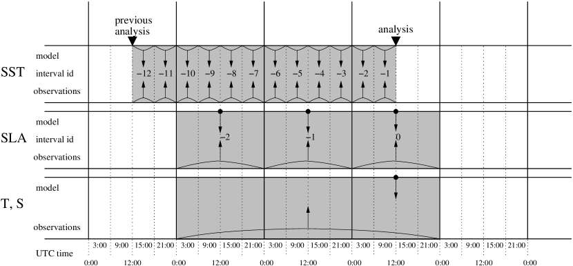
Figure 2.3: Example of observation timing in a MOM based ocean forecasting system.

From version 1.101.0 the code can check whether the time of the model dump used to calculate forecast observations matches the time of the (centre of the) corresponding observation window. To activate this check, one needs to add the name of the time variable in the model dump after the timing qualifier “c” or “e”. For the example above the first two sections of the observation types parameter file would the look as follows:

     NAME = SLA  VAR = eta_t  ISSURFACE = yes  ASYNCHRONOUS 1 C Time  <...>  NAME = SST  VAR = temp sstb  ISSURFACE = yes  ASYNCHRONOUS 0.25 E Time  <...>     

2.7 CALC

CALC is the second stage of data assimilation in EnKF-C. It calculates 2D arrays of local ensemble transforms $\mathbf{X}_{5}$ (for EnKF) or coefficients $\mathbf{w}$ (for EnOI).

The name of the binary for CALC is enkf_calc. It has the following usage and options:

     >./bin/enkf_calc    Usage: enkf_calc <prm file> [<options>]    Options:    --describe-prm-format [main|model|grid|obstypes]        describe format of a parameter file and exit    --forecast-stats-only        calculate and print forecast observation stats only    --ignore-no-obs        proceed even if there are no observations    --point-logs-only        skip calculating transforms for the whole grid and observation stats    --print-batch-stats         calculate and print global biases for each batch of observations    --print-memory-usage        print memory usage by each process    --single-observation-xyz <lon> <lat> <depth> <type> <inn> <std>        assimilate single observation with these parameters    --single-observation-ijk <fi> <fj> <fk> <type> <inn> <std>        assimilate single observation with these parameters    --use-existing-transforms        skip calculating ensemble transforms; use existing transforms*.nc files    --use-rmsd-for-obsstats        use RMSD instead of MAD when printing observation stats    --use-these-obs <obs file>        assimilate observations from this file; the file format must be compatible        with that of observations.nc produced by ‘enkf_prep’    --version        print version and exit    --write-HE        write ensemble observations to file "HE.nc"     

The option --forecast-stats-only can be used for quick calculation of the innovation statistics for a given background (or ensemble). This can be used, for example, for obtaining the persistence statistics, that is, the innovation statistics for the previous analysis.

The options --single-observation-xyz and --single-observation-ijk provide an easy way to conduct the so called single observation experiments, with the observation coordinates provided either in spatial or grid coordinates, correspondingly. Parameter <value> defines innovation rather than the observation value. Normally, this experiments would be conducted in the EnOI mode, calculating increment (option --output-increment of enkf_update) rather than analysis. When run in the EnKF mode, the increment (or analysis, depending on specifications) for each member is calculated.

Note that the calculated transforms do not incorporate inflation. Inflation is applied during UPDATE according to specifications (sec. 2.8.1).

2.7.1 Observation functions

Model estimations for observations of each type are calculated using observation functions specified for this type by entry HFUNCTIONS in the observation types parameter file, e.g.:

     NAME = SLA  ...  HFUNCTION = standard  ...     The available functions for each observation type are specified by the variable allhentries in calc/allhs.c. The “standard” functions do normally perform 2D or 3D linear interpolation from the corner model grid nodes for the cell containing the observation.

2.7.2 Interpolation of ensemble transforms

Local ensemble transforms $\mathbf{X}_{5}$ (EnKF) or local ensemble weights $\mathbf{w}$ (EnOI) represent smooth fields with the characteristic spatial variability scale of the localisation radius. This smoothness allows one to reduce the computational load in CALC by calculating local transforms or weights on a subgrid with a specified stride only, and using linearly interpolated transforms or weights in the intermediate grid cells (Yang et al., 2009). The value of the stride is defined by the STRIDE entry in the main parameter file and can be overwritten for a particular grid in the grid parameter file.

2.7.3 Adaptive moderation of observations

One of the standard QC procedures in DA is the so called background check, when an observation is compared with the forecast and discarded if the innovation magnitude exceeds some specified threshold. The downside of this approach is that it can not distinguish between situations of an outlier, big model error (e.g. because of an error in forcing), or model divergence. While one probably would like to discard an outlier, it is usually desirable to make use of valid observations, although, perhaps, with a reduced impact, to avoid “over-stressing” the model. In EnKF-C this is achieved by adaptive moderation of the observation impact by restricting the magnitude of the increment from a given observation in observation space by $K$ times magnitude of the spread of the forecast ensemble (Sakov and Sandery, 2017).

Specifically, the adaptive moderation of the observation impact is conducted by smoothly increasing the observation error depending on the magnitude of innovation as follows:

$$\sigma^{2}_{obs}\leftarrow\left[(\sigma_{f}^{2}+\sigma_{obs}^{2})^{2}+\sigma_{f}^{2}\,d^{2}/K^{2}\right]^{1/2}-\sigma_{f}^{2},$$

where $\sigma_{obs}$ is the observation error standard deviation, $\sigma_{f}$ – forecast ensemble spread, $d$ – innovation, and $K$ – the so called K-factor defined in the main parameter file (sec. 2.4.1). Tests with small models show that setting the $K\geq 2$ makes a marginal impact (if any) on performance of weakly suboptimal systems, while still can be quite beneficial in stressful situations.

2.7.4 Moderation of spread reduction

The moderating parameter $\alpha\in(0,1]$ specified in the main parameter file via the entry ALPHA allows one to reduce the contraction of ensemble during assimilation, while leaving the increment unchanged (“relaxation to prior spread”, Zhang et al. 2004, eq. 5). It modifies the right multiplied ensemble transform matrix as

$$\mathbf{T}_{R}\leftarrow\mathbf{I}+\alpha(\mathbf{T}_{R}-\mathbf{I}).$$

Setting $\alpha=0$ results in no update of the ensemble anomalies, while $\alpha=1$ results in full update.

2.7.5 Innovation statistics

In its course CALC calculates some basic innovation statistics: number of observations, mean absolute forecast innovation, mean absolute analysis innovation, mean forecast innovation, mean analysis innovation, mean forecast ensemble spread, and mean analysis ensemble spread. This statistics is provided for each region defined in the main parameter file (sec. 2.4.1), as well as for each time slot defined for asynchronous DA, and for each instrument. By default, EnKF-C defines one statistical region “Global” with domain $[x_{1},x_{2}]=[-999,999],[y_{1},y_{2}]=[-999,999]$.

In addition, for 3D observations CALC also calculates observation statistics in specified depth intervals. These intervals can be set via the entry ZSTATINTS in the grid parameter file; by default, three intervals are defined: [0 DEPTH_SHALLOW], [DEPTH_SHALLOW DEPTH_DEEP], and [DEPTH_DEEP DEPTH_MAX], where DEPTH_SHALLOW, DEPTH_DEEP and DEPTH_MAX are the macros defined in common/definitions.h.

Following is an example of innovation statistics written to the log (standard output) of enkf_calc:

       printing observation statistics:      region obs.type   # obs.  |for.inn.| |an.inn.|   for.inn.   an.inn.  for.spread  an.spread      ------------------------------------------------------------------------------------------      Tasman             SLA          3003    0.067      0.038      0.033      0.012      0.035      0.025              -4           712    0.058      0.038      0.035      0.013      0.028      0.021              -3           785    0.093      0.040      0.060      0.019      0.052      0.034              -2           700    0.062      0.043      0.030      0.016      0.027      0.021              -1           668    0.049      0.031      0.017      0.004      0.028      0.021               0           138    0.078      0.033     -0.043     -0.016      0.045      0.029               j1         1323    0.070      0.033      0.041      0.016      0.037      0.024               n1          876    0.073      0.042      0.052      0.025      0.036      0.026               g1          785    0.054      0.042     -0.004     -0.009      0.029      0.024               N/A          19    0.101      0.037      0.097      0.031      0.059      0.036             SST          9316    0.346      0.174     -0.215     -0.094      0.358      0.254              -4          2946    0.327      0.166     -0.236     -0.092      0.342      0.245              -3          2733    0.368      0.183     -0.270     -0.133      0.362      0.256              -2          2560    0.352      0.169     -0.167     -0.057      0.370      0.262              -1           580    0.342      0.191     -0.148     -0.093      0.414      0.291               0           497    0.305      0.182     -0.126     -0.075      0.307      0.225               AVHRR      9316    0.346      0.174     -0.215     -0.094      0.358      0.254             TEM           768    0.581      0.365     -0.245     -0.151      0.320      0.251               ARGO        768    0.581      0.365     -0.245     -0.151      0.320      0.251               0-50m       125    0.418      0.230      0.049      0.027      0.365      0.281               50-500m     451    0.678      0.403     -0.266     -0.141      0.360      0.278               >500m       192    0.458      0.365     -0.387     -0.291      0.196      0.170             SAL           768    0.079      0.060      0.014      0.019      0.033      0.028               ARGO        768    0.079      0.060      0.014      0.019      0.033      0.028               0-50m       125    0.079      0.063      0.031      0.035      0.034      0.030               50-500m     451    0.092      0.067      0.026      0.032      0.039      0.032               >500m       192    0.048      0.041     -0.027     -0.021      0.018      0.016     This excerpt shows innovation statistics for the region “Tasman”. It contains sections for SST, SLA and TEM observations. The summary statistics for each observation type is shown at the top of each section; then statistics for days -4, -3, -2, -1 and 0 of a 5-day DAW are shown for the two asynchronous types, SST and SLA. (More generally, the numbering of time intervals corresponds to their positions relative to the analysis time. For more details see sec. 2.6.3.) After that, statistics for particular instruments is shown; “N/A” corresponds to superobservations resulted from merging observations from two or more instruments. (From v1.115.0 there is no superobing across different instruments by default.) For subsurface temperature also statistics for shallow (0–50 m), deep ($>$500 m), and intermediate (50–500 m) observations is given.

The analysis innovation statistics is calculated from the updated (analysis) ensemble observations by CALC, thus avoiding the need to access analysis files produced later by UPDATE. The update of ensemble observations is performed in the same way as that of any other element of the state vector: for the EnKF – by applying the appropriate local ensemble transforms to the forecast ensemble observations,

$$\mathcal{H}(\mathbf{E}^{a})\leftarrow\mathcal{H}(\mathbf{E}^{f})\,\mathbf{X}_{5};$$

and for the EnOI – by applying the appropriate local linear combination of the ensemble observation anomalies:

$$\mathcal{H}(\mathbf{E}^{a})\leftarrow\left[\mathcal{H}(\mathbf{x}^{f})+(\mathbf{H}\mathbf{A}^{f})\mathbf{w}\right]\mathbf{1}^{\tiny\mathrm{T}}+\mathbf{H}\mathbf{A}^{f}.$$

CALC can be used for calculating forecast observation statistics only (via command line option --forecast-stats-only), without calculating transforms (EnKF) of update coefficients (EnOI). In the EnKF mode this regime involves calculating the statistics for the ensemble observation spread (and therefore parsing of the forecast ensemble), while in the EnOI mode it only calculates the statistics for the forecast innovation (and therefore does not need to access the ensemble).

2.7.6 Impact of observations

In the course of its work CALC routinely calculates two metrics for assessing the impact of observations, degrees of freedom of signal (DFS) and spread reduction factor (SRF):

$$\mathrm{DFS}=\mathrm{tr}(\mathbf{K}\mathbf{H})=\mathrm{tr}(\mathbf{G}\mathbf{S}),$$

$$\mathrm{SRF}=\sqrt{\frac{\mathrm{tr}(\mathbf{H}\mathbf{P}^{f}\mathbf{H}^{\tiny\mathrm{T}}\mathbf{R}^{-1})}{\mathrm{tr}(\mathbf{H}\mathbf{P}^{a}\mathbf{H}^{\tiny\mathrm{T}}\mathbf{R}^{-1})}}-1=\sqrt{\frac{\mathrm{tr}(\mathbf{S}^{\tiny\mathrm{T}}\mathbf{S})}{\mathrm{tr}(\mathbf{G}\mathbf{S})}}-1,$$

where $\mathrm{tr}(\cdot)$ is the trace function. The values of these metrics for each local analysis, calculated both for all observations and for observations of each type only, are written to file enkf_diag.nc. Note that the in EnKF-C DFS and SRF are calculated from the above expressions and represent theoretical values for the EnKF analysis; they coincide with the actual DFS and SRF values only for the ETKF, but not for the DEnKF, which is an approximation of the KF (and indeed not for the EnOI, which is not even an approximation).

In the EnKF context DFS is a useful indicator of potential rank problems. Normally, it should not exceed a fraction (a half, or better, a quarter) of the ensemble size per the characteristic time of the error growth. SRF shows the “strength” of DA. “Strong” DA implies a close to optimal system, which indeed never happens in practice. Therefore, ideally, SRF should be small (below 1, on average).

2.7.7 Multiple model grids

EnKF-C permits using multiple model grids, in which case the ensemble transforms are calculated sequentially for each of the grids. These transforms are then used for updating the model variables defined on the corresponding grids.

2.7.8 Domains

By default, all local observations for a given grid node contribute to the corresponding ensemble transform. Sometimes it is desirable to disconnect observations of certain type from contributing to transforms on particular grids. For example, it may be desirable in climate systems to disregard observations of the sea surface height in updating the atmospheric variables. The concept of “domains” introduced in v1.89.0 provides a mechanism for handling such situations within a single analysis. It works as follows. Each grid can be associated with a certain domain via the optional entry DOMAIN in the grid parameter file. For example, in a climate model one can have domains “Ocean” and “Atmosphere”. Then entry DOMAINS in the observation types parameter file can list domains observations of this type are visible from. By default, observations of any type are visible from all grids.

2.7.9 “Multi-scale” localisation

It is possible to specify the localisation taper function as a linear combination of the Gaspari and Cohn’s taper functions with different support radii:

$$f(r)=\sum_{i=1}^{N}w_{i}f_{0}(\frac{r}{R_{i}}),$$

where $w_{i}$ is the weight, $r$ is the distance, $R_{i}$ is the support radius, and

$$f_{0}(\frac{x}{2})=\left\{\begin{array}[]{ll}1-\frac{5}{3}x^{2}+\frac{5}{8}x^{3}+\frac{1}{2}x^{4}-\frac{1}{4}x^{5},&0\leq x\leq 1,\\ -\frac{2}{3}x^{-1}+4-5x+\frac{5}{3}x^{2}+\frac{5}{8}x^{3}-\frac{1}{2}x^{4}+\frac{1}{12}x^{5},&1<x\leq 2,\\ 0,&2<x.\end{array}\right.$$

This can be set by entries LOCRAD and LOCWEIGHT either in the main parameter file or in the observation types parameter file, e.g.:

  LOCRAD 150 500  LOCWEIGHT 0.9 0.1(recall that entries in the observation types parameter file for particular observation types override the common settings in the main parameter file). Note that the weights are normalised so that their sum is equal to 1.

2.8 UPDATE

UPDATE is the third and final stage of data assimilation in EnKF-C. It updates the ensemble (EnKF) or the background (EnOI) by applying the transforms calculated by CALC.

The name of the binary for UPDATE is enkf_update. It has the following usage and options:

     >./bin/enkf_update    Usage: enkf_update <prm file> [<options>]    Options:    --calculate-spread        calculate ensemble spread and write to spread.nc    --calculate-forecast-spread        calculate forecast ensemble spread only and write to spread.nc    --calculate-vertical-correlations        calculate correlation coefficients between surface and other layers of        3D variables and write to vcorr.nc    --calculate-vertical-correlations-only        as above, but exclude other (normally performed) jobs    --describe-prm-format [main|model|grid]        describe format of a parameter file and exit    --direct-write        write fields directly to the output file (default: write to tiles first)    --joint-output        append analyses to forecast files (default: write to separate files)    --leave-tiles        do not delete tiles    --no-fields-write        do not write analysis fields    --no-update        exclude tasks that require ensemble update    --output-increment        output analysis increment (default: output analysis)    --write-inflation        write adaptive inflation magnitudes to inflation.nc    --version        print version and exit     

The option --joint-output tells UPDATE to append analyses to the corresponding forecast files, using new variable names constructed by concatenating the forecast variable names and suffix _an. By default the analyses are written to separate files, using the same variable names as the forecast files, but with an extra suffix .analysis or .increment added to the file name, depending on whether the analysis or increment is written.

By default, UPDATE first writes each updated horizontal field of the model to a separate file (referred to here as a tile), and then concatenates these fields into analysis files. The tiles are removed after writing the analysis files; one may save time for allocating them on disk in the next cycle by leaving them on disk by using option --leave-tiles. This approach is somewhat less effective than direct writing to analysis files (without intermediate tiles), but, unfortunately, the direct writing is generally not reliable due to parallel I/O issues with NetCDF. Note that in some cases it proved to be possible to obtain robust performance with direct write using “classic” or “64-bit-offset” NetCDF formats.

2.8.1 Capping of inflation

Applying spatially uniform ensemble inflation involves areas with no local observations, where no assimilation is conducted. It can gradually inject energy into the model and deteriorate performance of the DAS over time. Similar problems may arise due to lack of correlation between some state elements updated with the same transforms, so that even in presence of local observations the ensemble spread for some elements may hardly reduce after assimilation, yet the ensemble anomalies are inflated.

To avoid this behaviour EnKF-C currently restricts inflation by specified fraction (1 by default) of the the spread reduction factor calculated directly for each element of the state vector during the update. For example, if inflation is specified as

INFLATION = 1.06 0.5then the ensemble anomalies for any model state element will be inflated by 6 %, but no more than $1+0.5(\sigma_{f}/\sigma_{a}-1)$, where $\sigma_{f}$ and $\sigma_{a}$ represent the forecast and analysis ensemble spreads for this element. Specification

INFLATION = 1.06is equivalent to

INFLATION = 1.06 1Capping inflation by the magnitude of reduction of the ensemble spread is the default in EnKF-C; to revert to the uniform inflation add qualifier PLAIN to the entry INFLATION in the main parameter file, e.g.:

INFLATION = 1.06 PLAINThe common inflation settings in the main parameter file can be overwritten by settings for particular model variables specified in the model parameter file (sec. 2.4.2).

2.9 Hybrid covariance

From v2.0.0 EnKF-C makes it possible using hybrid state error covariance by combining covariances from the EnKF ensemble and an ensemble of static anomalies (sec. 1.7). This option is activated by specifying METHOD = HYBRID in the main parameter file, the directory of the static ensemble, and the mixing coefficient GAMMA (see sec. 2.4.1).

When the method is set to “hybrid”, the forecast ensemble spread written in the innovation statistics summary at the end of CALC is that of the combined ensemble (1.50), but the analysis innovation spread is that of the dynamic ensemble only. The forecast and analysis ensemble spread fields written by UPDATE when specifying options --calculate-spread, --calculate-forecast-spread, and --calculate-forecast-spread-only are calculated using the dynamic ensemble anomalies only. In contrast, the vertical correlations (UPDATE options --calculate-vertical-correlations and --calculate-vertical-correlations-only) are calculated using the full ensemble.

Note that setting GAMMA = 0 makes the hybrid system formally equivalent to the EnKF (but not numerically, because of the roundoff errors), while setting ENSSIZE_DYNAMIC = 1 makes it formally equivalent to the EnOI.

2.10 DA tuning

Following are the main parameters for DAS tuning in EnKF-C:

• R-factors;

• inflation magnitudes;

• localisation radii.

The R-factors can be defined for each observation type. They represent scaling coefficients for the corresponding observation error variances and affect the impact of these observations: increasing R-factor decreases the impact of observations and vice versa. Specifying R-factor equal $k$ produces the same increment as reducing the ensemble spread by $k^{1/2}$ times.

The main parameter file defines the base R-factor common for all observation types. It is possible to specify additional R-factors for observations of each type (sec. 2.4.4); the resulting R-factor for an observation is then given by multiplication of the common R-factor and the additional R-factor specified for observations of this type.

Multiplicative inflation can be seen as an additional forgetting factor in the KF. In EnKF-C one can specify the inflation multiple for analysed ensemble anomalies, e.g.:

     > grep INFLATION main.prm  INFLATION = 1.05 PLAIN  > grep temp -A 1 model.prm  VAR = temp  INFLATION = 1.07 PLAIN     In this case all model variables except “temp” will have inflation of 5 %, while “temp” will have inflation of 7 %. The ability to define different inflation rates for different variables can be useful for non-dynamical variables, such as estimated biases, helping to avoid the ensemble collapse for them. In general, to retain dynamical balances one should rather avoid using different inflation magnitudes across model variables. Note that even small inflation can substantially affect the ensemble spread established in the course of evolution of the system. By default EnKF-C applies adaptive capping of inflation (sec. 2.8.1).

Localisation radius is defined by the entry LOCRAD in the parameter file. Specifically, this entry defines the support localisation radius (in km). This is different to the “effective” localisation radius, which is defined sometimes as $e^{1/2}\approx 1.65$ - folding distance. For the Gaspary and Cohn’s taper function used in EnKF-C the effective radius is approximately 3.5 times smaller than the support radius.

Increasing the localisation radius increases the number of local observations and hence the overall impact of observations. To compensate this in a system with horizontal localisation one has to change the R-factor as the square of the localisation radius.

From v1.77.0 it is possible to limit the maximal number of local observations of each observation type via the entry NLOBSMAX in the main parameter file (sec. 2.4.1). This common setting can be overriden for particular observation types in the observation types parameter file (sec. 2.4.4). Note that using this setting can result in discontinuity of the analysis because the set of observations used for local analyses in adjacent grid cells can change in a discontinuous way. Also, it forces sorting of the local observations, which can substantially increase the search time. Therefore the general advise is to avoid using this functionality except perhaps interpolation oriented products.

2.11 Point logs

It is often desirable to investigate the drivers of the analysis or, more generally, certain features of the DAS and their behaviour over time. In practice such investigations can be logistically complicated due to limitations on storage and/or access to it. Yet, it is usually feasible to save the model state and observations for a number of specified locations.

EnKF-C provides capability of saving complete DA related information for specified horizontal locations in so called “point logs”. The locations are specified in the main parameter file, e.g.:

POINTLOG 94.3 134.1POINTLOG 78.39 111.7Here the information will be saved for points with geographic coordinates (94.3,134.1), (78.39, 111.7) in files pointlog_94.300,134.100.nc, pointlog_78.390,111.700.nc, and so on. By default the ensemble trsansforms and all forecast and analysis state variables existing at these locations are saved; however, if an optional grid name is specified as the third paramater of the POINTLOG entry, e.g.

POINTLOG 94.3 134.1 t-gridthen only transforms and variables for this grid are saved.

Following is an example of point log file header (file pointlog_156.000,-32.000.nc from example 4):

     netcdf pointlog_156.000\,-32.000 {  dimensions:          m1 = 96 ;          m2 = 96 ;          p = 1444 ;          p-0 = 1444 ;          p-1 = 1444 ;  variables:          int obs_ids(p) ;          float lcoeffs(p) ;          float lon(p) ;          float lat(p) ;          float depth(p) ;          float obs_val(p) ;          float obs_estd(p) ;          float obs_fi(p) ;          float obs_fj(p) ;          float obs_fk(p) ;          int obs_type(p) ;                  obs_type:SLA = 0 ;                  obs_type:RFACTOR_SLA = 2. ;                  obs_type:LOCRAD_SLA = 200. ;                  obs_type:WEIGHT_SLA = 1. ;                  obs_type:GRIDID_SLA = 0 ;                  obs_type:SST = 1 ;                  obs_type:RFACTOR_SST = 4. ;                  obs_type:LOCRAD_SST = 200. ;                  obs_type:WEIGHT_SST = 1. ;                  obs_type:GRIDID_SST = 0 ;                  obs_type:TEM = 2 ;                  obs_type:RFACTOR_TEM = 8. ;                  obs_type:LOCRAD_TEM = 800. ;                  obs_type:WEIGHT_TEM = 1. ;                  obs_type:GRIDID_TEM = 0 ;                  obs_type:SAL = 3 ;                  obs_type:RFACTOR_SAL = 8. ;                  obs_type:LOCRAD_SAL = 800. ;                  obs_type:WEIGHT_SAL = 1. ;                  obs_type:GRIDID_SAL = 0 ;          int obs_inst(p) ;                  obs_inst:j1 = 0 ;                  obs_inst:n1 = 1 ;                  obs_inst:ESACCI = 2 ;                  obs_inst:WindSat = 3 ;                  obs_inst:ARGO = 4 ;                  obs_inst:CTD = 5 ;                  obs_inst:TAO = 6 ;                  obs_inst:PIRATA = 7 ;                  obs_inst:CARS62 = 8 ;          float obs_time(p) ;                  obs_time:units = "days from days from 6565.5 days since 1990-01-01" ;          int grid-0 ;                  grid-0:id = 0 ;                  grid-0:name = "t-grid" ;                  grid-0:domain = "Default" ;                  grid-0:fi = 49.5 ;                  grid-0:fj = 49.5 ;                  grid-0:nk = 2 ;                  grid-0:model_depth = 4642.25f ;          int grid-1 ;                  grid-1:id = 1 ;                  grid-1:name = "c-grid" ;                  grid-1:domain = "Default" ;                  grid-1:fi = 48.9999694824219 ;                  grid-1:fj = 49.0000076293945 ;                  grid-1:nk = 2 ;                  grid-1:model_depth = NaNf ;          float s-0(p-0) ;          float S-0(m2, p-0) ;          double X5-0(m1, m2) ;                  X5-0:long_name = "ensemble transform calculated for location                       (fi,fj)=(49.500,49.500) on grid 0 (\"t-grid\")" ;          float s-1(p-1) ;          float S-1(m2, p-1) ;          double X5-1(m1, m2) ;                  X5-1:long_name = "ensemble transform calculated for location                       (fi,fj)=(49.000,49.000) on grid 1 (\"c-grid\")" ;          float eta_t(m2) ;                  eta_t:gridid = 0 ;                  eta_t:INFLATION = 1.1f, 1.f ;          float eta_t_an(m2) ;          float temp(nk-0, m2) ;                  temp:gridid = 0 ;                  temp:INFLATION = 1.1f, 1.f ;          float temp_an(nk-0, m2) ;          float salt(nk-0, m2) ;                  salt:gridid = 0 ;                  salt:INFLATION = 1.1f, 1.f ;          float salt_an(nk-0, m2) ;          float u(nk-1, m2) ;                  u:gridid = 1 ;                  u:INFLATION = 1.1f, 1.f ;          float u_an(nk-1, m2) ;          float v(nk-1, m2) ;                  v:gridid = 1 ;                  v:INFLATION = 1.1f, 1.f ;          float v_an(nk-1, m2) ;    // global attributes:                  :version = "2.0.17" ;                  :lon = 156. ;                  :lat = -32. ;                  :MODE = "EnKF" ;                  :SCHEME = "DEnKF" ;                  :ALPHA = 1. ;                  :ngrids = 2 ;  }     

This data makes it possible to check DA algorithms by reproducing the ensemble transforms (for EnKF) or weights (for EnOI) calculated by EnKF-C from $\mathbf{S}$ and $\mathbf{s}$ according to section 1.3.3; restore observations from $\mathbf{s}$ by using the corresponding R-factors and localisation coefficients; to monitor the ensemble spread for each model variable; calculate inflation applied to the analysed anomalies; calculate impacts of particular observations; and so on.

Note that in a multi-domain setting (sec. 2.7.8) the number of local observations seen on a particular grid (e.g. p-0) can be smaller than the total number of local observations $p$. In this case to get the local observations on this grid one needs to filter out observations of types defined on domains other than the domain the grid belongs to.

2.12 Use of innovation statistics for model validation

EnKF-C can calculate innovation statistics for validating a model against observations only, without data assimilation. The pre-requisites are (i) observations and (ii) model dump readable by the code, and possibly (iii) auxiliary files for projecting the model state to observation space (e.g. grid specs and mean SSH). To get the innovation statistics one needs to:

• set up the parameter files in a normal way (MODE = EnOI), omitting the ensemble directory and assimilation related parameters;

• run enkf_prep;

• run enkf_calc with additional parameter --forecast-stats-only.

The results will be written to the log of enkf_calc. An example of using this functionality is available by running make stats in examples/1 (see sec. 2.3).

2.13 Bias correction

It is possible to estimate and correct bias for a model variable with the EnKF by generating and using an ensemble of bias fields. These bias fields need to be subtracted from the corresponding observation forecasts. This is accomplished by specifying a secondary variable in the observation type entry VAR and by passing the name of this variable to the corresponding observation (H-) functions, which need to take care for subtracting the bias from the model forecasts. As of v1.98.0, there are two such H-functions: H_surf_biased() identified by entry “biased” in observation types paramater file, and H_subsurf_wsurfbias(), identified by entry “wsurfbias”. (The latter applies surface bias field to the mixed layer.)

Because bias fields are usually assumed to persist (not change) during propagation, one may need to make specific settings for their inflation to avoid their collapse (loss of spread) over time. Another possibility is to introduce a “forgetting” stochastic model for bias fields, for example:

$$\mathbf{x}_{i+1}=\lambda\,\mathbf{x}_{i}+(1-\lambda^{2})^{1/2}\boldsymbol{\sigma},$$

where $\lambda$ is the forgetting factor, $0<\lambda<1,\;1-\lambda\ll 1$, and $\boldsymbol{\sigma}\sim\sigma_{0}N(0,1)$, where $\sigma_{0}$ is the error standard deviation of $\mathbf{x}$. This can be specified for a model variable via entry RANDOMISE in the corresponding section of the model parameter file (sec. 2.4.2).

2.14 Assimilation in log space

The entry APPLYLOG in the model parameter file makes it possible to conduct assimilation for a variable in log space. This means that a transform with log10 function will be applied to model values and observations before DA, and the inverse transform with pow10 will be applied after DA. This option can be applied only for positive variables.

To apply log10/pow10 transforms in EnOI or Hybrid modes (MODE = ENOI or MODE = HYBRID) is only possible if the static ensemble is in logarithmic space. This must be confirmed by the user by using option --allow-logspace-with-static-ens.

When APPLYLOG is specified, the ensemble spread and ensemble vertical correlations are calculated for the transformed variable.

2.15 System issues

2.15.1 Compiler flags

Following is a brief description of the compiler flags in EnKF-C.

INTERNAL_QSORT_R (enkf_prep, enkf_calc) Uses internal code for qsort_r(). Has to be defined for compiling on Mac OS platforms.

SHUFFLE_ROWS (enkf_calc) Supposed to produce more latitudinally uniform load between CPUs. Currently, because transforms for each row of the grid are sent to the master process for writing, this option effectively makes no difference to performance, I believe.

USE_SHMEM (enkf_calc) Uses shared memory for storing ensemble observations, which much reduces the memory footprint in CALC. From v1.110.0 also uses shared memory for storing grid K-D trees and observation K-D trees. Requires MPI-3. This is a default option, but can be unset, particularly for smaller systems, when memory is not an issue.

MINIMISE_ALLOC (enkf_calc) Pre-allocates arrays in CALC to reduce potential problems with memory fragmentation. This is a default option from v1.103.0.

OBS_SHUFFLE (enkf_calc) Randomly shuffles observations before parsing them into K-D trees. Potentially this can substantially improve performance in the case of spatially ordered observations (not verified).

TW_VIAFILE (enkf_calc) Communicate ensemble transforms via files. Use this option if MPI communication becomes clogged.

DEFLATE_ALL (enkf_calc, enkf_update) Apply specified NetCDF deflation to all NetCDF files, including ensemble transforms, spread, inflation, and various tiles. This can save some disk space, but slows down i/o.

NCW_SKIPSINGLE (enkf_update) Skips “normal” (not unlimited) “inner” dimensions of length one when copying definitions of variables from one NetCDF file to another.

2.15.2 Memory footprint

To reduce the memory footprint, most of the potentially large arrays in EnKF-C use float data type.

The following table lists the most memory-wise important objects.

Object	Typical size1	PREP	CALC	UPDATE
observation array	6 GB	•
super-observation array2	1.5 GB	•	•
ensemble observations2 $\mathcal{H}(\mathbf{E})$	5 GB $\times$ 2		•
single grid2,3	0.4 GB	•	•
observation K-D trees2	0.85 GB		•
one 3D model field	1 GB		•
ensemble of one horizontal field	2 GB			•
transform array (I/O, EnKF only)	22 GB4			•

⁽¹⁾ for EnKF/OFAM3 system ($3600\times 1500\times 51$ grid, 96 members, $5\cdot 10^{7}$ observations, $1.3\cdot 10^{7}$ super-observations)
⁽²⁾ stored in shared memory (one instance per compute node)
⁽³⁾ when defined as a curvilinear grid
⁽⁴⁾ with STRIDE = 3

The memory footprint of PREP is defined by the size of the observation structure array and, in some cases, by curvilinear grids. The memory usage by curvilinear grids is much reduced by parsing them into K-D trees (default from v1.101.4; the only option since v1.106.0) rather than into binary trees. Because PREP is not parallelised (mainly due to lack of robust parallel analogue of qsort procedure), in practice its memory footprint is rarely a problem.

The footprint of CALC is mainly defined by the size of ensemble observations $\mathcal{H}(\mathbf{E})$. From version 1.74, it has been substantially reduced for multi-core CPUs by storing only one instance of ensemble observations per compute node. This involves using the shared memory and requires MPI-3.

For the EnKF, the footprint of UPDATE is mainly defined by the size of the array of simultaneously updated horizontal model fields. The number of simultaneously updated fields is defined by parameter FIELDBUFFERSIZE. Note that larger values of FIELDBUFFERSIZE increase computational effectiveness by reducing the number of reads of and interpolations within $\mathbf{X}_{5}$ arrays. For the EnOI, the footprint of UPDATE is insensitive to FIELDBUFFERSIZE (which should be set to 1), and is defined by the size of the ensemble of horizontal model fields.

2.15.3 Exit action

When exiting on an error, EnKF-C by default prints the stack trace, which allows to trace the exit location in the code. Another option – to generate a segmentation fault – can be activated by setting EXITACTION = SEGFAULT in the parameter file. Note that when run on multiple processors, this can result in segmentation faults on more than one processor (but not necessarily on every engaged processor, as some processes can also be forced to exit by MPI_abort()). If the system is set to generate core dumps, they can indeed be used for investigating the final state of the program.

2.15.4 Dependencies and compilation issues

Compiling EnKF-C requires the following external libraries:

• netcdf;

• lapack (or mkl_rt);

• openmpi;

EnKF-C also relies on qsort_r(), which may be lacking in older systems. In such cases use compile flag -DINTERNAL_QSORT_R to activate the internal version of this procedure.

Notes:

1. Using Intel’s version of Lapack library – Intel Math Kernel Library – can improve performance over Lapack compiled with gfortran.

2.16 Possible problems / FAQ

1. The code does not compile on OS X platform.

   In some cases compiler can not find qsort_r(). Edit Makefile by adding -DINTERNAL_QSORT_R to PREPCALC_FLAGS.

   In other cases compiler can not find definition of data type __compar_d_fn_t. Add line

     typedef int (*__compar_d_fn_t) (const void*, const void*, void*);to common/definitions.h.

2. In the innovation stats report at the tail of CALC log I get some entries “N/A” for instrument tags.

   These entries show stats for super-observations obtained by collating observations from different instruments. To avoid collating such observations run PREP with option
   --no-superobing-across-instruments. This became default from v1.115.0.

3. CALC becomes too slow after increasing localisation radius

   This is due to the increased number of local observations. One way to reduce it is to run superobing on a virtual coarser horizontal grid by increasing parameter SOBSTRIDE from the default value of 1 to 2 or more.

4. CALC starts calculating transforms swiftly, but then slows down almost to a standstill.

   This can happen with large systems when the MPI communication becomes clogged. Recompile CALC with flag -DTW_VIAFILE to communicate transforms via filesystem.

5. In UPDATE I am getting error
   “<...> "spread.nc": <...> NC_UNLIMITED size already in use”.

   UPDATE tries to create a common output file for all model variables. This may be not straightforward due to possible differences in formats of various model data files involved. Try compiling UPDATE with flag -DNCW_SKIPSINGLE.

Abbreviations

CL	-	covariance localisation
DEnKF	-	deterministic EnKF
DA	-	data assimilation
DAS	-	data assimilation system
DAW	-	data assimilation window
DFS	-	degrees of freedom of signal
EKF	-	extended Kalman filter
EnKF	-	ensemble Kalman filter
EnOI	-	ensemble optimal interpolation
ETKF	-	ensemble transform Kalman filter
ETM	-	ensemble transform matrix
FGAT	-	first guess at appropriate time
KF	-	Kalman filter
KS	-	Kalman smoother
LA	-	local analysis
QC	-	quality control
SDAS	-	state of data assimilation system
SRF	-	spread reduction factor
SVD	-	singular value decomposition

Symbols

General symbols

$\mathbf{x}$ (small, bold)	-	a vector
$\mathbf{1}$	-	a vector with all elements equal to 1
$\mathbf{0}$	-	a vector with all elements equal to 0
$\mathbf{A}$ (capital, bold)	-	a matrix
$\mathbf{I}$	-	an identity matrix
$\mathbf{U}$	-	a unitary matrix, $\mathbf{U}\mathbf{U}^{\tiny\mathrm{T}}=\mathbf{I}$
$\mathbf{A}^{\tiny\mathrm{T}}$	-	transposed matrix $\mathbf{A}$
$\mathbf{A}^{1/2}$	-	the unique positive definite square root of a positive definite matrix $\mathbf{A}$
$\mathbf{A}(m_{1}:m_{2},n_{1}:n_{2})$	-	the block of $\mathbf{A}$ composed of rows from $m_{1}$ to $m_{2}$ and columns from $n_{1}$ to $n_{2}$
$\mathrm{tr}(\mathbf{A})$	-	trace of $\mathbf{A}$
$\mathcal{H}\circ\mathcal{M}(\mathbf{x})$	-	$\mathcal{H}\left[\mathcal{M}(\mathbf{x})\right]$
$\mathbf{A}\circ\mathbf{B}$	-	by-element, or Hadamard, or Schur product of matrices
$\|\mathbf{x}\|^{2}_{\mathbf{B}}$	-	$\mathbf{x}^{\tiny\mathrm{T}}\mathbf{B}\mathbf{x}$

DA related symbols

$m$	-	ensemble size
$n$	-	state size
$p$	-	number of observations
$\mathbf{A}$	-	ensemble anomalies, $\mathbf{A}=\mathbf{E}-\mathbf{x}\mathbf{1}^{\tiny\mathrm{T}}$
$\mathbf{E}$	-	ensemble
$\mathbf{G}$	-	an intermediate matrix in the EnKF analysis, $\mathbf{G}\equiv(\mathbf{I}+\mathbf{S}^{\tiny\mathrm{T}}\mathbf{S})^{-1}\mathbf{S}^{\tiny\mathrm{T}}=\mathbf{S}^{\tiny\mathrm{T}}(\mathbf{I}+\mathbf{S}\mathbf{S}^{\tiny\mathrm{T}})^{-1}$
$\mathcal{H}$	-	nonlinear observation operator; in linear case – affine observation operator
$\mathbf{H}$	-	linearised observation operator, $\mathbf{H}=\nabla\mathcal{H}(\mathbf{x})$
$J$	-	cost function
$\mathcal{M}$	-	nonlinear model operator; in linear case – affine model operator
$\mathbf{M}$	-	linearised model operator, $\mathbf{M}=\nabla\mathcal{M}(\mathbf{x})$
$\mathbf{P}$	-	state error covariance estimate; also used as abbreviation for $\mathbf{A}\mathbf{A}^{\tiny\mathrm{T}}/(m-1)$
$\mathbf{Q}$	-	model error covariance
$\mathbf{R}$	-	observation error covariance
$\mathbf{S}$	-	normalised ensemble observation anomalies, $\mathbf{S}=\mathbf{R}^{-1/2}\mathbf{HA}/\sqrt{m-1}$
$\mathbf{T}_{L}$	-	left-multiplied ensemble transform matrix, $\mathbf{A}^{a}=\mathbf{T}_{L}\mathbf{A}^{f}$
$\mathbf{T}_{R}$	-	right-multiplied ensemble transform matrix, $\mathbf{A}^{a}=\mathbf{A}^{f}\mathbf{T}_{R}$
$\mathbf{U}^{p}$	-	a unitary mean-preserving matrix, $\mathbf{U}^{p}(\mathbf{U}^{p})^{\tiny\mathrm{T}}=\mathbf{I}$, $\mathbf{U}^{p}\mathbf{1}=\mathbf{1}$
$\mathbf{X}_{5}$	-	historic symbol for the full ensemble transform matrix, $\mathbf{E}^{a}=\mathbf{E}^{f}\mathbf{X}_{5}$
$\mathbf{s}$	-	normalised innovation, $\mathbf{s}=\mathbf{R}^{-1/2}\left[\mathbf{y}-\mathcal{H}(\mathbf{x}^{f})\right]/\sqrt{m-1}$
$\mathbf{x}$	-	state estimate
$\mathbf{y}$	-	observation vector
$\mathbf{w}$	-	vector of linear coefficients for updating the mean, $\mathbf{x}^{a}=\mathbf{x}^{f}+\mathbf{A}^{f}\mathbf{w}$
$(\cdot)^{f}$	-	forecast expression
$(\cdot)^{a}$	-	analysis expression
$(\cdot)_{i}$	-	either expression at cycle $i$ or $i$th element of a vector
$\accentset{i}{(\cdot)}$	-	local expression for state element $i$
$\accentset{\{o\}}{(\cdot)}$	-	local expression for observation $o$

References

- Andrews (1968) Andrews, A., 1968: A square root formulation of the Kalman covariance equations. AIAA J., 6, 1165–1168.
- Bishop et al. (2001) Bishop, C. H., B. Etherton, and S. J. Majumdar, 2001: Adaptive sampling with the ensemble transform Kalman filter. part I: theoretical aspects. Mon. Wea. Rev., 129, 420–436.
- Evensen (1994) Evensen, G., 1994: Sequential data assimilation with a nonlinear quasi-geostrophic model using Monte-Carlo methods to forecast error statistics. J. Geophys. Res., 99, 10143–10162.
- Evensen (2003) — 2003: The Ensemble Kalman Filter: theoretical formulation and practical implementation. Ocean Dynam., 53, 343–367.
- Evensen (2004) — 2004: Sampling strategies and square root analysis schemes for the EnKF. Ocean Dynam., 54, 539–560.
- Evensen and van Leeuwen (2000) Evensen, G. and P. J. van Leeuwen, 2000: An ensemble Kalman smoother for nonlinear dynamics. Mon. Wea. Rev., 128, 1852–1867.
- Gaspari and Cohn (1999) Gaspari, G. and S. E. Cohn, 1999: Construction of correlation functions in two and three dimensions. Q. J. R. Meteorol. Soc., 125, 723–757.
- Hamill and Whitaker (2001) Hamill, T. M. and J. S. Whitaker, 2001: Distance-dependent filtering of background error covariance estimates in an ensemble Kalman filter. Mon. Wea. Rev., 129, 2776–2790.
- Houtekamer and Mitchell (2001) Houtekamer, P. L. and H. L. Mitchell, 2001: A sequential ensemble Kalman filter for atmospheric data assimilation. Mon. Wea. Rev., 129, 123–137.
- Hunt et al. (2004) Hunt, B. R., E. Kalnay, E. J. Kostelich, E. Ott, D. J. Patil, T. Sauer, I. Szunyogh, J. A. Yorke, and A. V. Zimin, 2004: Four-dimensional ensemble Kalman filtering. Tellus, 56A, 273–277.
- Hunt et al. (2007) Hunt, B. R., E. J. Kostelich, and I. Szunyogh, 2007: Efficient data assimilation for spatiotemporal chaos: A local ensemble transform Kalman filter. Physica D, 230, 112–126.
- Kalman (1960) Kalman, R. E., 1960: A new approach to linear filtering and prediction problems. J. Basic. Eng., 82, 35–45.
- Oke et al. (2008) Oke, P. R., G. B. Brassington, D. A. Griffin, and A. Schiller, 2008: The Bluelink ocean data assimilation system (BODAS). Ocean Model., 21, 46–70.
- Ott et al. (2003, rev. 2005) Ott, E., B. R. Hunt, I. Szunyogh, A. V. Zimin, E. J. Kostelich, M. Corazza, E. Kalnay, D. J. Patil, and J. A. Yorke, 2003, rev. 2005: A local ensemble Kalman filter for atmospheric data assimilation. http://arxiv.org/abs/physics/0203058.
- Sakov and Bertino (2011) Sakov, P. and L. Bertino, 2011: Relation between two common localisation methods for the EnKF. Comput. Geosci., 15, 225–237.
- Sakov et al. (2012) Sakov, P., F. Counillon, L. Bertino, K. A. Lisæter, P. R. Oke, and A. Korablev, 2012: TOPAZ4: an ocean-sea ice data assimilation system for the North Atlantic and Arctic. Ocean Science, 8, 633–656.
- Sakov et al. (2010) Sakov, P., G. Evensen, and L. Bertino, 2010: Asynchronous data assimilation with the EnKF. Tellus, 62A, 24–29.
- Sakov and Oke (2008a) Sakov, P. and P. R. Oke, 2008a: A deterministic formulation of the ensemble Kalman filter: an alternative to ensemble square root filters. Tellus, 60A, 361–371.
- Sakov and Oke (2008b) — 2008b: Implications of the form of the ensemble transformations in the ensemble square root filters. Mon. Wea. Rev., 136, 1042–1053.
- Sakov and Sandery (2017) Sakov, P. and P. Sandery, 2017: An adaptive quality control procedure for data assimilation. Tellus A, 69, 1318031.
- Verlaan and Heemink (1997) Verlaan, M. and A. W. Heemink, 1997: Tidal flow forecasting using reduced rank square root filters. Stoch. Hydrol. Hydraul., 11, 349–368.
- Yang et al. (2009) Yang, S.-C., E. Kalnay, B. Hunt, and E. N. Bowler, 2009: Weight interpolation for efficient data assimilation with the Local Ensemble Transform Kalman Filter. Q. J. R. Meteorol. Soc., 135, 251–262.
- Zhang et al. (2004) Zhang, F., C. Snyder, and J. Sun, 2004: Impacts of initial estimate and observation availability on convective-scale data assimilation with an ensemble Kalman filter. Mon. Wea. Rev., 132, 1238–1253.