Abstract

An important ingredient for applications of nuclear physics to e.g. astrophysics or nuclear energy are the cross sections for reactions of neutrons with rare isotopes. Since direct measurements are often not possible, indirect methods like $(d,p)$ reactions must be used instead. Those $(d,p)$ reactions may be viewed as effective three-body reactions and described with Faddeev techniques. An additional challenge posed by $(d,p)$ reactions involving heavier nuclei is the treatment of the Coulomb force. To avoid numerical complications in dealing with the screening of the Coulomb force, recently a new approach using the Coulomb distorted basis in momentum space was suggested. In order to implement this suggestion, one needs not only to derive a separable representation of neutron- and proton-nucleus optical potentials, but also compute the Coulomb distorted form factors in this basis.
Keywords: Separable representation of optical potentials, momentum space Coulomb distorted form factors, Coulomb without screening

1 Introduction

Nuclear reactions are an important probe to learn about the structure of unstable nuclei. Due to the short lifetimes involved, direct measurements are usually not possible. Therefore indirect measurements using ($d,p$) reactions have been proposed (see e.g. Refs. [1, 2, 3]). Deuteron induced reactions are particularly attractive from an experimental perspective, since deuterated targets are readily available. From a theoretical perspective they are equally attractive because the scattering problem can be reduced to an effective three-body problem [4]. Traditionally deuteron-induced single-neutron transfer ($d,p$) reactions have been used to study the shell structure in stable nuclei, nowadays experimental techniques are available to apply the same approaches to exotic beams (see e.g. [5]). Deuteron induced $(d,p)$ or $(d,n)$ reactions in inverse kinematics are also useful to extract neutron or proton capture rates on unstable nuclei of astrophysical relevance. Given the many ongoing experimental programs worldwide using these reactions, a reliable reaction theory for $(d,p)$ reactions is critical.

One of the most challenging aspects of solving the three-body problem for nuclear reactions is the repulsive Coulomb interaction. While the Coulomb interaction for light nuclei is often a small correction to the problem, this is certainly not the case for intermediate mass and heavy systems. Over the last decade, many theoretical efforts have focused on advancing the theory for $(d,p)$ reactions (e.g. [6, 7]) and testing existing methods (e.g. [8, 4, 9]). Currently, the most complete implementation of the theory is provided by the Lisbon group [10], which solves the Faddeev equations in the Alt, Grassberger and Sandhas [11] formulation. The method introduced in [10] treats the Coulomb interaction with a screening and renormalization procedure as detailed in [12, 13]. While the current implementation of the Faddeev-AGS equations with screening is computationally effective for light systems, as the charge of the nucleus increases technical difficulties arise in the screening procedure [14]. Indeed, for most of the new exotic nuclei to be produced at the Facility of Rare Isotope Beams, the current method is not adequate. Thus one has to explore solutions to the nuclear reaction three-body problem where the Coulomb problem is treated without screening.

In Ref. [6], a three-body theory for $(d,p)$ reactions is derived with explicit inclusion of target excitations, where no screening of the Coulomb force is introduced. Therein, the Faddeev-AGS equations are cast in a Coulomb-distorted partial-wave representation, instead of a plane-wave basis. This approach assumes the interactions in the two-body subsystems to be separable. While in Ref. [6] the lowest angular momentum in this basis ($l=0$) is derived for a Yamaguchi-type nuclear interaction is derived as analytic expression, it is desirable to implement more general form factors, which are modeled after the nuclei under consideration.

In order to bring the three-body theory laid out in Ref. [6] to fruition, well defined preparatory work needs to be successfully carried out. Any momentum space Faddeev-AGS type calculation needs as input transition matrix elements in the different two-body subsystems. In the case of ($d,p$) reactions with nuclei these are the $t$-matrix elements obtained from the neutron-proton, the neutron-nucleus and proton-nucleus interactions. Since the formulation in Ref. [6] is designed for separable interactions, those need to be developed not only in the traditionally employed plane wave basis, but also the basis of Coulomb scattering states.

This contribution summarizes the three major developments required to provide reliable input to the three-body formulation for $(d,p)$ reactions without screening the Coulomb force, namely

• the derivation of momentum-space separable representations of neutron-nucleus optical potentials [15],

• the derivation of momentum-space separable representations of proton-nucleus optical potentials in the Coulomb basis [16],

• the calculation of neutron-nucleus form-factors in the basis of momentum-space Coulomb scattering states [17].

Sections 2, 3, and 4 summarize the necessary steps to achieve reliable calculations of those input quantities needed for three-body calculations that treat the Coulomb force without screening. Finally, we summarize in Section 5.

2 Separable Representation of Nucleon-Nucleus
Optical Potentials

Separable representations of the forces between constituents forming the subsystems in a Faddeev approach have a long tradition in few-body physics. There is a large body of work on separable representations of nucleon-nucleon (NN) interactions (see e.g. Refs. [18, 19, 20, 21, 22]) or meson-nucleon interactions [23, 24]. In the context of describing light nuclei like ⁶He [25] and ⁶Li [26] in a three-body approach, separable interactions have been successfully used. A separable nucleon-¹²C optical potential was proposed in Ref. [27], consisting of a rank-1 Yamaguchi-type form factor fitted to the positive energies and a similar term describing the bound states in the nucleon-¹²C configuration. However, systematic work along this line for heavy nuclei, for which excellent phenomenological descriptions exist in terms of Woods-Saxon functions [28, 29, 30, 31] has not been carried out until recently [15].

The separable representation of two-body interactions suggested by Ernst-Shakin-Thaler [32] (EST) is well suited for achieving this goal. We note that this EST approach has been successfully employed to represent NN potentials [18, 19]. However, the EST scheme derived in Ref. [32], though allowing energy dependence of the potentials [33, 34], assumes that they are Hermitian. Therefore, we generalized the EST approach in Ref. [15] in order to be applicable for optical potentials which are complex. For the ease of the reader, we briefly summarize the main points of that work.

For applications to the theory of nuclear reactions all potential operators $U$ need to satisfy

$${\cal K}U{\cal K}^{-1}=U^{\dagger},$$ (1)

where $\cal{K}$ is the time reversal operator appropriate to the system. This condition guarantees that the $S$-matrix corresponding to $U$ is symmetric and that reaction amplitudes constructed from these potentials satisfy reciprocity relations. When $U$ is a central potential in the space of a spinless particle, $\cal{K}$ can be chosen to be the anti-linear complex conjugation operator ${\cal K}_{0}$, which in the coordinate space basis $|{\bf r}\rangle$ is defined by

$${\cal K}_{0}\;\alpha\,|{\bf r}\rangle=\alpha^{*}({\cal K}_{0}|{\bf r}\rangle)=\alpha^{*}|{\bf r}\rangle,$$ (2)

and from which we deduce ${\cal K}_{0}|{\bf p}\rangle=|-{\bf p}\rangle.$ Note that for this particular ${\cal K}$ we have $({\cal K}_{0})^{-1}={\cal K}_{0}$.

Considering first a rank-1 separable potential, the EST scheme presented in Ref. [32] requires that a separable potential ${\bf U}$ leads to the same scattering wave functions at a specific energy $E_{k_{E}}$ (support point) as the potential $u$ it is supposed to represent. For $u$ being a non-Hermitian potential, we define

$${\bf U}(E_{k_{E}})\equiv\frac{u|f_{l,k_{E}}\rangle\langle f^{*}_{l,k_{E}}|u}{\langle f^{*}_{l,k_{E}}|u|f_{l,k_{E}}\rangle}\equiv u|f_{l,k_{E}}\rangle{\hat{\lambda}}\langle f^{*}_{l,k_{E}}|u\;,$$ (3)

where the strength parameter is defined by $({\hat{\lambda}})^{-1}=\langle f^{*}_{l,k_{E}}|u|f_{l,k_{E}}\rangle$. Here $f_{l,k_{E}}(r)$ is the unique regular radial wave function corresponding to $u$ and $f^{*}_{l,k_{E}}(r)$ is the unique regular radial wavefunction corresponding to $u^{*}$. By a suitable choice of arbitrary normalization constants we can arrange that $f^{*}_{l,k_{E}}(r)$ is simply the complex conjugate of $f_{l,k_{E}}$ and hence ${\cal K}_{0}|f_{l,k_{E}}\rangle=|f^{*}_{l,k_{E}}\rangle$.

If $u$ satisfies ${\cal K}_{0}u{\cal K}_{0}=u^{\dagger}$ the definition of Eq. (3) gives a symmetric complex potential matrix that satisfies

$${\cal K}_{0}{\bf U}(E_{k_{E}}){\cal K}_{0}=\left[\vphantom{f^{*}_{l,k_{E}}}{\cal K}_{0}u|f_{l,k_{E}}\rangle\right]({\hat{\lambda}})^{*}\left[\langle f^{*}_{l,k_{E}}|u{\cal K}_{0}\right]=u^{\dagger}|f^{*}_{l,k_{E}}\rangle({\hat{\lambda}})^{*}\langle f_{l,k_{E}}|u^{\dagger}=U^{\dagger},$$ (4)

where the square brackets mean that ${\cal K}_{0}$ here acts only on the quantities within the brackets.

In analogy to the procedure followed in Ref. [32] we define a complex separable potential of arbitrary rank in a given partial wave as

$${\bf U}=\sum_{i,j}u|f_{l,k_{E_{i}}}\rangle\langle f_{l,k_{E_{i}}}|M|f^{*}{{}_{l},k_{E_{j}}}\rangle\langle f^{*}_{l,k_{E_{j}}}|u.$$ (5)

Here $f_{l,k_{E_{i}}}$ and $f^{*}_{l,k_{E_{i}}}$ are the same unique regular radial wave function as used in Eq. (3). Note that $u$ may also be energy dependent.

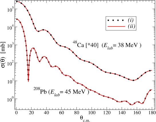
Figure 1: The unpolarized differential cross section for elastic scattering of neutrons from ⁴⁸Ca (upper) and ²⁰⁸Pb (lower) as function of the c.m. angle. For ⁴⁸Ca the cross section is calculated at a laboratory kinetic energy of 38 MeV and is scaled by a factor 40. The calculation for ²⁰⁸Pb is carried out at $E_{lab}$ = 45 MeV. The solid lines ($ii$) depict the cross section calculated in momentum space based on the rank-5 separable representation of the CH89 [28] phenomenological optical potential, while the dotted lines ($i$) represent the corresponding coordinate space calculations.

The matrix $M$ is defined and constrained by

$$\delta_{ik} = \sum_{j}\langle f_{l,k_{E_{i}}}|M|f^{*}_{l,k_{E_{j}}}\rangle\langle f^{*}_{l,k_{E_{j}}}|u|f_{l,k_{E_{k}}}\rangle$$ (6)

$$= \sum_{j}\langle f^{*}_{l,k_{E_{i}}}|u|f_{l,k_{E_{j}}}\rangle\langle f_{l,k_{E_{j}}}|M|f^{*}_{l,k_{E_{k}}}\rangle.$$ (7)

The corresponding separable partial wave $t$-matrix must be of the form

$$t(E)=\sum_{i,j}u|f_{l,k_{E_{i}}}\rangle\tau_{ij}(E)\langle f^{*}_{l,k_{E_{j}}}|u\;,$$ (8)

with the following restrictions

$$\delta_{nj} =\sum_{i}\langle f^{*}_{l,k_{E_{n}}}|u-ug_{0}(E)u|f_{l,k_{E_{i}}}\rangle\;\tau_{ij}(E),$$ (9)

$$\delta_{ik} =\sum_{j}\tau_{ij}(E)\;\langle f^{*}_{l,k_{E_{j}}}|u-ug_{0}(E)u|f_{l,k_{E_{k}}}\rangle.$$ (10)

For the explicit calculation of the matrix $\tau_{ij}(E)$, we define a matrix

$$R_{ij}(E)\equiv\langle f^{*}{{}_{l},k_{E_{i}}}|u-ug_{0}(E)u|f_{l,k_{E_{j}}}\rangle,$$ (11)

so that the condition of Eq. (10) reads

$$\sum_{j}\tau_{ij}(E)R_{jk}(E)=\delta_{ik},$$ (12)

from which follows

$$\tau_{ij}(E)=\left(R(E)\right)^{-1}_{ij}.$$ (13)

Using that $t(p^{\prime},k_{E_{i}},E_{i})=\langle f^{*}_{l,k_{E_{i}}}|u|p^{\prime}\rangle$, and $t(p,k_{E_{i}},E_{i})=\langle p|u|f_{l,k_{E_{i}}}\rangle$, the matrix elements $R_{ij}$ are calculated in momentum space as given explicitly in Ref. [15].

In order to demonstrate the construction of a separable representation of a complex potential we apply the generalized EST scheme to neutron scattering from ⁴⁸Ca and ²⁰⁸Pb and use as starting point the Chapel Hill phenomenological global optical potential CH89 [28], which has been widely used in the literature over the last decades. Like most phenomenological global optical potentials, CH89 is based on Woods-Saxon functions, which are more naturally given in coordinate space, and have an explicit energy dependence in the strength functions. In order to derive a separable momentum-space representation of CH89, we first must construct a momentum-space representation of the potential itself. The Fourier transform of Woods-Saxon functions leads to a series expansion in momentum space, of which only the first two terms are necessary to obtain a converged result [15]. The momentum-space potential then enters a Lippmann-Schwinger (LS) integral equation to obtain the half-shell t-matrices at fixed energies (support points) $E_{i}$, from which the separable representation given in Eq. (8) is then constructed after having obtained the coupling matrix $\tau_{ij}(E)$ from the solution of Eq. (13).

Table 1: The EST support points at c.m. energies $E_{k_{i}}$ used for constructing the separable representation of the partial wave s-matrix of the n$+^{48}$Ca and n$+^{208}$Pb systems. The support points in the last row for the n$+^{208}$Pb system given in bold face indicate the universal set of support points, which can be used to construct a representation for all nuclei given by the CH89 [28] phenomenological optical potential.

system	partial wave(s)	rank	EST support point(s) [MeV]
	$l\geq 10$	1	40
n$+^{48}$Ca	$l\geq 8$	2	29, 47
	$l\geq 6$	3	16, 36, 47
	$l\geq 0$	4	6, 15, 36, 47
	$l\geq 16$	1	40
n$+^{208}$Pb	$l\geq 13$	2	35, 48
	$l\geq 11$	3	24, 39, 48
	$l\geq 6$	4	11, 21, 36, 45
	$\mathbf{l\geq 0}$	$\mathbf{5}$	$\mathbf{5,11,21,36,47}$

A major finding of Ref. [15] is a systematic classification of support points for partial wave groups, so that the partial wave S-matrix elements are reproduced to at least four significant figures compared to the original momentum-space solution of the LS equation. It turns out that the low partial waves of the $n+^{208}$Pb system require a rank-5 separable potential to be well represented in the energy regime between 0 and 50 MeV center-of-mass energy. The rank required for achieving a good representation decreases with increasing angular momentum of the partial wave considered. The recommendation of Ref. [15] for both the rank and the locations of the support points to be used when describing medium-mass and heavy systems generated from the CH89 potential are repeated in Table 1 for the convenience of the reader.

In order to demonstrate the quality of the separable representations obtained with the generalized EST scheme, Fig. 1 depicts the unpolarized differential cross section for elastic scattering of neutrons from ⁴⁸Ca at 38 MeV laboratory kinetic energy and from ²⁰⁶Pb at 45 MeV as function of the center-of-mass (c.m.) angle $\theta_{c.m.}$. The solid lines ($i$) represent the calculations with the separable representations, while the dotted lines ($ii$) stand for the corresponding coordinate space calculations. The agreement is excellent over the entire angular range, indicating that all partial wave S-matrix elements that enter the cross section are well described by the separable representation.

3 Separable Representation of Proton-Nucleus
Optical Potentials in the Coulomb Basis

In order to implement the formulation of the Faddeev-AGS equations proposed in Ref. [6] we need the proton-nucleus form factors in the Coulomb distorted basis, and thus need to have a separable representation of proton-nucleus optical potentials. In Refs. [35, 36] rank-1 separable interactions of Yamaguchi form were introduced to represent the nuclear force up to a few MeV, and the Coulomb distorted basis was introduced to compute proton elastic scattering from light nuclei. This is not sufficient for considering the proton-nucleus interaction in a separable representation for scattering of heavy nuclei up to tens of MeV. Thus we need to extend the generalization of the EST scheme presented in the previous section such that it can be applied in the Coulomb distorted basis [16].

In general the scattering between a proton and a nucleus is governed by a potential

$$w=v^{c}+u^{s},$$ (14)

where $v^{c}$ is the repulsive Coulomb potential and $u^{s}$ an arbitrary short range potential. In general $u^{s}$ consists of an optical potential, which describes the nuclear interactions and a short-ranged Coulomb potential traditionally parameterized as the potential of a charged sphere with radius $R_{0}$ from which the point Coulomb force is subtracted [28]. In practice,

$$u^{s}=u^{N}+(v^{cd}-v^{c}),$$ (15)

where $u^{N}$ represents the nuclear (optical) potential, $v^{cd}$ is the Coulomb potential inside the nucleus, and is usually taken as the Coulomb potential for a uniformly charged sphere of radius $R_{0}$, from which the point Coulomb potential is subtracted. The expressions for the short-ranged charge distribution is given in Ref. [28] as

$$(v^{cd}-v^{c})(r)=\alpha Z_{1}Z_{2}\left[\frac{1}{2R_{0}}\left(3-\frac{r^{2}}{R_{0}^{2}}\right)-\frac{1}{r}\right],$$ (16)

with $Z_{1}$ and $Z_{2}$ being the atomic numbers of the particles, and $\alpha$ the Coulomb coupling constant. Since the scattering problem governed by the point Coulomb force has an analytic solution, the scattering amplitude for elastic scattering between a proton and a spin-zero nucleus is obtained as the sum of the Rutherford amplitude $f^{C}(E_{p_{0}},\theta)$ and the Coulomb distorted nuclear amplitude given by

$$M^{CN}(E_{p_{0}},\theta)=f^{CN}(E_{p_{0}},\theta)+{\hat{\sigma}}\cdot\mathbf{\hat{n}}\;g^{CN}(E_{p_{0}},\theta),$$ (17)

with

$$f^{CN}(E_{p_{0}},\theta)=$$

$$-\pi\mu\sum_{l=0}^{\infty}e^{2i\sigma_{l}(E_{p_{0}})}P_{l}(\cos\theta)\times\Big{[}(l+1)\langle p_{0}|\tau^{CN}_{l+}(E_{p_{0}})|p_{0}\rangle+l\langle p_{0}|\tau^{CN}_{l-}(E_{p_{0}})|p_{0}\rangle\Big{]},$$

and

$$g^{CN}(E_{p_{0}},\theta)=$$

$$-\pi\mu\sum_{l=0}^{\infty}e^{2i\sigma_{l}(E_{p_{0}})}P^{1}_{l}(\cos\theta)\times\Big{[}\langle p_{0}|\tau^{CN}_{l+}(E_{p_{0}})|p_{0}\rangle-\langle p_{0}|\tau^{CN}_{l-}(E_{p_{0}})|p_{0}\rangle\Big{]}.$$

Here $E_{p_{0}}=p_{0}^{2}/2\mu$ is the center-of-mass (c.m.) scattering energy which defines the on-shell momentum $p_{0}$, and $\sigma_{l}=\;\arg\Gamma(1+l+i\eta)$ is the Coulomb phase shift. The Sommerfeld parameter is given by $\eta=\alpha Z_{1}Z_{2}\mu/p_{0}$. The unit vector $\mathbf{\hat{n}}$ is normal to the scattering plane, and ${\hat{\sigma}}/2$ is the spin operator. The subscripts ${}^{\prime}+^{\prime}$ and ${}^{\prime}-^{\prime}$ correspond to a total angular momentum $j=l+1/2$ and $j=l-1/2$.

Suppressing the total angular momentum indices for simplicity, the Coulomb distorted nuclear $t$-matrix element is given by $\langle p_{0}|\tau^{CN}_{l}(E_{p_{0}})|p_{0}\rangle$, which is the solution of a LS type equation,

$$\langle p|\tau^{CN}_{l}(E_{p_{0}})|p_{0}\rangle=\langle p|u^{s}_{l}|p_{0}\rangle\\ +\int p^{\prime 2}dp^{\prime}\langle p|u^{s}_{l}|p^{\prime}\rangle\langle p^{\prime}|g_{c}(E_{p_{0}}+i\varepsilon)|p^{\prime}\rangle\langle p^{\prime}|\tau^{CN}_{l}(E_{p_{0}})|p_{0}\rangle.$$ (20)

Here

$$g_{c}^{-1}(E_{p_{0}}+i\varepsilon)=E_{p_{0}}+i\varepsilon-H_{0}-v^{c}$$ (21)

is the Coulomb Green’s function and $H_{0}$ the free Hamiltonian. The Coulomb distorted nuclear $t$-matrix element $\langle p|\tau^{CN}_{l}(E_{p_{0}})|p_{0}\rangle$ is related to the proton-nucleus $t$-matrix $\langle p|t_{l}(E_{p_{0}})|p_{0}\rangle$ by the familiar two-potential formula

$$\langle p|t_{l}(E_{p_{0}})|p_{0}\rangle=\langle p|t^{C}_{l}(E_{p_{0}})|p_{0}\rangle+e^{2i\sigma_{l}(E_{p_{0}})}\langle p|\tau^{CN}_{l}(E_{p_{0}})|p_{0}\rangle,$$ (22)

where $\langle p|t^{C}_{l}(E_{p_{0}})|p_{0}\rangle$ is the point Coulomb $t$-matrix. When the integral equation, Eq. (20), is solved in the basis of Coulomb eigenfunctions, $g_{c}$ acquires the form of a free Green’s function and the difficulty of solving it is shifted to evaluating the potential matrix elements in this basis. For deriving a separable representation of the Coulomb distorted proton-nucleus $t$-matrix element, we generalize the approach suggested by Ernst, Shakin, and Thaler (EST) [32], to the charged particle case. The basic idea behind the EST construction of a separable representation of a given potential is that the wave functions calculated with this potential and the corresponding separable potential agree at given fixed scattering energies $E_{i}$, the EST support points. The formal derivations of [32] use the plane wave basis, which is standard for scattering involving short-range potentials. However, the EST scheme does not depend on the basis and can equally well be carried out in the basis of Coulomb scattering wave functions.

In order to generalize the EST approach to charged-particle scattering, one needs to be able to obtain the scattering wave functions or half-shell t-matrices from a given potential in the Coulomb basis, and then construct the corresponding separable representation thereof.

In order to calculate the half-shell $t$-matrix of Eq. (3), we evaluate the integral equation in the Coulomb basis as suggested in [37] and successfully applied in [38], and note that in this case the Coulomb Green’s function behaves like a free Green’s function. Taking $|\Phi_{l,p}^{c}\rangle$ to represent the partial wave Coulomb eigenstate, the LS equation becomes

$$\langle\Phi_{l,p}^{c}|\tau^{CN}_{l}(E_{p_{0}})|\Phi_{l,p_{0}}^{c}\rangle = \langle\Phi_{l,p}^{c}|u^{s}|\Phi_{l,p_{0}}^{c}\rangle+$$ (23)

$$\int\limits_{0}^{\infty} \langle\Phi_{l,p}^{c}|u^{s}|\Phi_{l,p^{\prime}}^{c}\rangle\;\frac{p^{\prime 2}dp^{\prime}}{E_{p_{0}}-E_{p^{\prime}}+i\varepsilon}\langle\Phi_{l,p^{\prime}}^{c}|\tau^{CN}_{l}(E_{p_{0}})|\Phi_{l,p_{0}}^{c}\rangle$$ (24)

$$\equiv \langle p|\tau^{CN}_{l}(E_{p_{0}})|p_{0}\rangle,$$ (25)

which defines the Coulomb distorted nuclear $t$-matrix of Eq. (20).

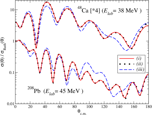
Figure 2: The unpolarized differential cross section for elastic scattering of protons from ⁴⁸Ca (upper) and ²⁰⁸Pb (lower) divided by the Rutherford cross section as function of the c.m. angle $\theta_{c.m.}$. For ⁴⁸Ca the cross section is calculated at a laboratory kinetic energy of 38 MeV and is scaled by a factor 4. The calculation for ²⁰⁸Pb is carried out at $E_{lab}$ = 45 MeV. The solid lines ($i$) depict the cross section calculated in momentum space based on the rank-5 separable representation of the CH89 [28] phenomenological optical potential, while the dotted lines ($ii$) represent the corresponding coordinate space calculations. The dash-dotted lines ($iii$) show calculations in which the short-ranged Coulomb potential is omitted.

To determine the short-range potential matrix element, we follow Ref. [37] and insert a complete set of position space eigenfunctions

$$\langle\Phi_{l,p^{\prime}}^{c}|u^{s}_{l}|\Phi_{l,p}^{c}\rangle = \frac{2}{\pi}\int\limits_{0}^{\infty}\langle\Phi_{l,p^{\prime}}^{c}|r^{\prime}\rangle\;r^{\prime 2}dr^{\prime}\;\langle r^{\prime}|u^{s}_{l}|r\rangle\;r^{2}dr\;\langle r|\Phi_{l,p}^{c}\rangle$$ (26)

$$= \frac{2}{\pi p^{\prime}p}\int\limits_{0}^{\infty}rr^{\prime}drdr^{\prime}\;F_{l}(\eta^{\prime},p^{\prime}r^{\prime})\;\langle r^{\prime}|u^{s}_{l}|r\rangle\;F_{l}(\eta,pr).$$ (27)

The partial wave Coulomb functions are given in coordinate space as

$$\langle r|\Phi_{l,p}^{c}\rangle\equiv\frac{F_{l}(\eta,pr)}{pr},$$ (28)

where $F_{l}(\eta,pr)$ are the standard Coulomb functions [39], and $\eta$($\eta^{\prime}$) is the Sommerfeld parameter determined with momentum $p$($p^{\prime}$).

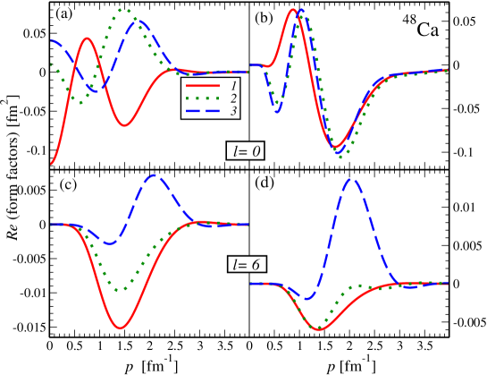
Figure 3: The real parts of the partial wave neutron form factors for ⁴⁸Ca as function of the momentum $p$ for $l=0$ (a) and $l=6$ (c). The form factors are calculated at the energies indicated in Table 1 for the given angular momentum, $1\equiv$ 6 MeV, $2\equiv$ 15 MeV, and $3\equiv$ 36 MeV. The real parts of the proton form factors for ⁴⁸Ca as function of the momentum $p$ are given for $l=0$ in (b) and $l=6$ in (d) for the energies indicated in Table 1.

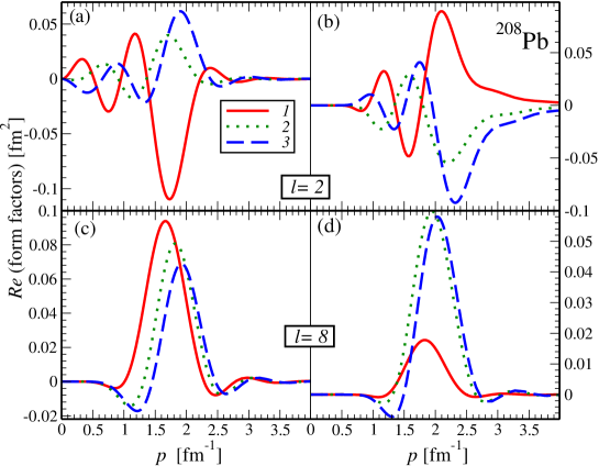
Figure 4: The real parts of the partial wave neutron form factors for ²⁰⁸Pb as function of the momentum $p$ for $l=0$ (a) and $l=8$ (c). The form factors are calculated at the first three energies indicated in Table 1 for the given angular momentum, $1\equiv$ 21 MeV, $2\equiv$ 36 MeV, and $3\equiv$ 47 MeV ($l=2$) and 45 MeV ($l=8$). The real parts of the proton form factors for ²⁰⁸Pb as function of the momentum $p$ are given for $l=0$ in (b) and $l=8$ in (d) for the same energies.

For our application we consider phenomenological optical potentials of Woods-Saxon form which are local in coordinate space. Thus the momentum space potential matrix elements simplify to

$$\langle\Phi_{l,p^{\prime}}^{c}|u^{s}_{l}|\Phi_{l,p}^{c}\rangle=\frac{2}{\pi p^{\prime}p}\int\limits_{0}^{\infty}dr\;F_{l}(\eta^{\prime},p^{\prime}r)u^{s}_{l}(r)F_{l}(\eta,pr).$$ (29)

We compute these matrix elements for the short-range piece of the CH89 phenomenological global optical potential [28], which consists of the nuclear part parameterized in terms of Woods-Saxon functions and the short-range Coulomb force of Eq. (16). The integral of Eq. (29) can be carried out with standard methods, since $u^{s}(r)$ is short ranged and the coordinate space Coulomb wavefunctions are well defined. The accuracy of this integral can be tested by replacing the Coulomb functions with spherical Bessel functions and comparing the resulting matrix elements to the partial-wave decomposition of the semi-analytic Fourier transform used for the calculations in the previous Section. For the cases we studied a maximum radius of 14 fm, 300 grid points are sufficient to obtain matrix elements with a precision of six significant digits.

Extending the EST separable representation to the Coulomb basis involves replacing the neutron-nucleus half-shell $t$-matrix in Eqs. (7)-(9) by the Coulomb distorted nuclear half-shell $t$-matrix. This leads to the separable Coulomb distorted nuclear $t$-matrix

$$\tau^{CN}_{l}(E_{p_{0}})=\sum_{i,j}u^{s}|f^{c}_{l,k_{E_{i}}}\rangle\;\tau^{c}_{ij}(E_{p_{0}})\;\langle{f^{c}}^{*}_{l,k_{E_{j}}}|u^{s},$$ (30)

with $\tau^{c}_{ij}(E_{p_{0}})$ being constrained by

$$\sum_{i}\langle{f^{c}}^{*}_{l,k_{E_{n}}}|u^{s}-u^{s}g_{c}(E_{p_{0}})u^{s}|f^{c}_{l,k_{E_{i}}}\rangle\tau^{c}_{ij}(E)=\delta_{nj}$$ (31)

$$\sum_{j}\tau^{CN}_{ij}(E_{p_{0}})\;\langle{f^{c}}^{*}_{l,k_{E_{j}}}|u^{s}-u^{s}g_{c}(E_{p_{0}})u^{s}|f^{c}_{l,k_{E_{k}}}\rangle=\delta_{ik}\;.$$

Here $|f^{c}_{l,k_{E_{i}}}\rangle$ and $|{f^{c}}^{*}_{l,k_{E_{i}}}\rangle$ are the regular radial scattering wave functions corresponding to the short range potentials $u^{s}$ and $(u^{s})^{*}$ at energy $E_{i}$. The separable Coulomb distorted nuclear $t$-matrix elements are given by

$$\langle p^{\prime}|\tau^{CN}_{l}(E_{p_{0}})|p\rangle \equiv \sum_{i,j}h_{l,i}^{c}(p^{\prime})\tau^{c}_{ij}(E_{p_{0}})h_{l,j}^{c}(p)$$ (32)

$$= \sum_{i,j}\langle\Phi_{l,p^{\prime}}^{c}|u^{s}|f^{c}_{l,k_{E_{i}}}\rangle\tau^{c}_{ij}(E_{p_{0}})\langle{f^{c}}^{*}_{l,k_{E_{j}}}|u^{s}|\Phi_{l,p}^{c}\rangle,$$ (33)

where the form factor

$$h_{l,i}^{c}(p) \equiv \langle\Phi_{l,p}^{c}|u^{s}|f^{c}_{l,k_{E_{i}}}\rangle$$

$$= \langle{f^{c}}^{*}_{l,k_{E_{i}}}|u^{s}|\Phi_{l,p}^{c}\rangle=\langle p|\tau^{CN}_{l}(E_{i})|k_{E_{i}}\rangle$$

is the Coulomb distorted short-range half-shell $t$-matrix satisfying Eq. (25). We want to point out that the generalization of the EST scheme to complex potentials is not affected by changing the basis from plane waves to Coulomb scattering states.

For studying the quality of the representation of proton-nucleus optical potentials we consider p+⁴⁸Ca and p+²⁰⁸Pb elastic scattering and show the unpolarized differential cross sections divided by the Rutherford cross section as function of the c.m. angle $\theta_{c.m.}$ in Fig. 2. First, we observe very good agreement in both cases of the momentum space calculations using the separable representation with the corresponding coordinate space calculations. Second, we want to point out that we used for the separable representation of the proton-nucleus partial-wave $t$-matrices the same support points (Table 1) as in the neutron-nucleus case. This makes the determination of suitable support points $E_{i}$ for a given optical potential and nucleus quite efficient. In Fig. 2 we also show a calculation in which the short-range Coulomb potential of Eq. (3) is omitted. The differences in the cross sections clearly demonstrate the importance of including this term. A detailed comparison of the partial-wave S-matrix elements as function of the angular momentum is given in Ref. [16].

In order to illustrate some details of the separable representation of the $t$-matrix of Eq. (8) that leads to the cross section given in Fig. 1, we display in the left panels of Fig. 3 the real parts of the form factors of the $n+^{48}$Ca $t$-matrix for $l=0$ (a) and $l=6$ (c) at support points given in Table 1 for the respective angular momentum. Only for $l=0$ the form factors have a finite value at $p=0$, while for the higher angular momentum all form factors go to zero for $p\rightarrow 0$ due to the angular momentum barrier. For comparison, the right panels in Fig. 3 display the form factors of the Coulomb distorted nuclear $t$-matrix from Eq. (20) for $p+^{48}$Ca for the same angular momenta and support points. Those $t$-matrix elements enter the calculation of the cross section in Fig. 2. First we note that for $l=0$ the $p+^{48}$Ca form factors are quite different from the $n+^{48}$Ca form factors. In addition, they fall off much slower as function of $p$, a property mainly caused by the short range Coulomb potential.

In Fig. 4 we carry out an analogous comparison between the form factors for the $n+^{208}$Pb and $p+^{208}$Pb form factors. Here the energies are chosen slightly higher, since in the $p+^{208}$Pb the form factors at the lowest energies given in Table 1 are very small. The slow decrease of the $p+^{208}$Pb form factor for the small angular momentum is even more pronounced in this case.

At this point it is crucial to note that in Figs. 3 and 4 we compare two quite different form factors. For $n+^{48}$Ca and $n+^{208}$Pb scattering the $t$-matrix elements leading to the form factors are calculated as described in Section 2 using as basis states in- and out-going plane-wave scattering states. For $p+^{48}$Ca and $p+^{208}$Pb, the Coulomb distorted nuclear $t$-matrix elements enter the cross section and lead to the form factors. Those Coulomb distorted $t$-matrix elements are evaluated in the basis of Coulomb scattering states. Thus, one should not be surprised that the form factors given in the left and right panels of Figs 3 and 4 differ from each other.

4 Coulomb distorted Neutron-Nucleus Form
Factors

In order to treat charged-particle scattering in momentum space without employing a screening procedure for the Coulomb force, it is necessary to formulate the scattering problem in a momentum space Coulomb basis. For proton-nucleus scattering, a two-body problem with a repulsive Coulomb force, the Coulomb distorted nuclear matrix elements are already derived in this bases, as described in the previous Section and Refs. [16, 37, 38]. When moving forward to $(d,p)$ reactions, an effective three-body problem with two charged particles, one needs to solve generalized Faddeev-AGS equations in Coulomb basis, as was proposed in Ref. [6]. In order for this approach to be numerically practical, reliable techniques to calculate expectation values in this basis must exist. Here we evaluate the neutron-nucleus form factors from Section 2 in the Coulomb basis to illustrate the feasibility of the approach.

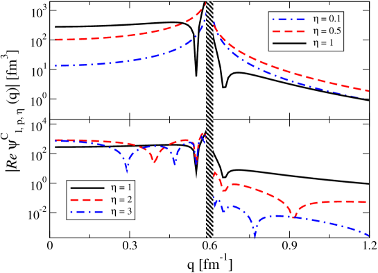
Figure 5: The absolute value of the real part of the $l=0$ Coulomb wave function $\psi^{C}_{l,p,\eta}(p)$ for the external momentum $p=0.6$ fm^-1 and $\eta=0.1,0.5,1$ (upper panel) and $\eta=1,3,3$ (lower panel), as function of $q$. The shaded area masks the function around the singularity at $p\rightarrow q$, where it is highly oscillatory.

The starting point is the analytic expression for the Coulomb wave function in momentum space which, after a partial wave decomposition, can be written as (see [40] and Ref. [17])

$$\psi^{C}_{l,p}(q)\,=\,-\,\frac{2\pi\,e^{\eta\pi/2}}{pq}\,\lim_{\gamma\to+0}\,\frac{d}{d\gamma}\left\{\left[\frac{q^{2}-(p+i\gamma)^{2}}{2pq}\right]^{i\eta}\,(\zeta^{2}-1)^{-i\frac{\eta}{2}}\,Q_{l}^{i\eta}(\zeta)\right\}\;.$$ (35)

Here, $p$ is the magnitude of the fixed asymptotic momentum and $\zeta=(p^{2}+q^{2}+\gamma^{2})/2pq$. The Sommerfeld parameter is given as $\eta=Z_{1}Z_{2}e^{2}\mu/p$ where $Z_{1}=1$ and $Z_{2}$ corresponds to the number of protons in the nucleus, and $\mu$ is the reduced mass of the two-body system under consideration. The spherical function $Q_{l}^{i\eta}(\zeta)$ in Eq. (35) can be expressed in terms of hypergeometric functions ${}_{2}F_{1}$ [41]. However, care must be taken in its evaluation, since there are specific limits of validity of the various expansions. Specific difficulties together with the expressions implemented in this work are discussed in detail in Refs. [17, 42].

In Fig. 5 we display $l=0$ partial wave Coulomb functions for fixed external momentum $q=0.6$ fm ^-1 as function of $p$ for selected values of $\eta$. The functions exhibit oscillatory singular behavior for $p\rightarrow q$. This region is indicated in the figure by the shaded band. For values of $\eta\geq 1$ oscillatory behavior is already present way outside the singular region. It is also worthwhile to note that once the momentum $p$ is larger than the external momentum $q$, the magnitude of the Coulomb function falls off by at least an order of magnitude.

For evaluating the neutron-nucleus form factors in the Coulomb basis, we start from the separable partial-wave $t$-matrix operator given in Eq. (8). Evaluating its momentum space matrix elements $\langle p|t_{l}(E)|p^{\prime}\rangle$ in a plane-wave basis gives the nuclear form factors

$$\langle p|u|f_{l,k_{E}}\rangle = t_{l}(p,k_{E};E_{k_{E}})\equiv u_{l}(p)$$

$$\langle f^{*}_{l,k_{E}}|u|p^{\prime}\rangle = t_{l}(p^{\prime},k_{E};E_{k_{E}})\equiv u_{l}(p^{\prime}),$$ (36)

where the $t_{l}(p,k_{E};E_{k_{E}})$ are the half-shell two-body t-matrices obtained as solution of a momentum space LS equation with the complex potential $u$.

The corresponding Coulomb-distorted form factors are obtained by replacing the plane-wave basis state by a Coulomb basis state $|\psi^{C}_{l,p}\rangle$ leading to

$$\langle\psi^{C}_{l,p}|u|f_{l,k_{E}}\rangle = \int_{0}^{\infty}\frac{dq\;q^{2}}{2\pi^{2}}\;u_{l}(q)\psi^{C}_{l,p}(q)^{\star}\equiv u^{C}_{l}(p)$$ (37)

$$\langle f^{*}_{l,k_{E}}|u|\psi^{C}_{l,p}\rangle = \int_{0}^{\infty}\frac{dq\;q^{2}}{2\pi^{2}}\;u_{l}(q)\;\psi^{C}_{l,p}(q)\equiv u^{C}_{l}(p)^{\dagger}$$ (38)

When $\eta\rightarrow 0$, Eqs.(37) and (38) tend to Eq.(36). This expression is a generalization of the form introduced in Ref. [6] to account for complex interactions.

The main challenge in computing the integrals of Eq. (37) and (38) is the oscillatory singularity in the integrand for $q=p$, which is of the form

$$S(q-p)=\lim_{\gamma\to+0}\frac{1}{(q-p+i\gamma)^{1+i\eta}}.$$ (39)

This type of singularity cannot be numerically evaluated by the familiar principal value subtractions but rather needs to be treated using the scheme of Gel’fand and Shilov [43], as proposed by [6, 41]. The generalization to the complex form factors of our application is given in Ref. [17]. The essence of the Gel’fand and Shilov scheme is to subtract as many terms as needed of the Laurent expansion in a small region around the pole so that the oscillations around the pole become small, and the integral becomes regular. For further details of the calculations as well as numerical tests we refer to Ref. [17].

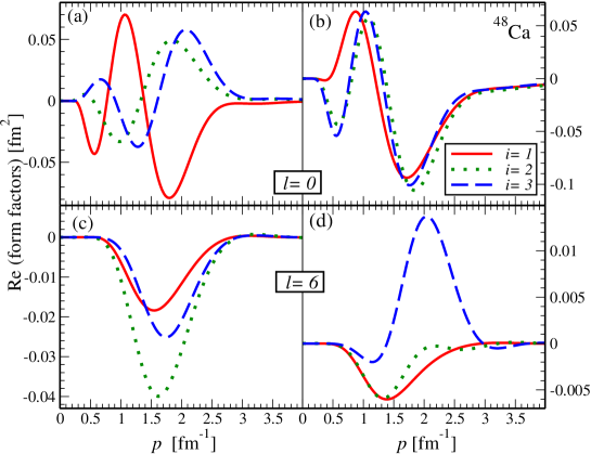
Figure 6: The real parts of the partial wave Coulomb distorted neutron form factors for ⁴⁸Ca as function of the momentum $p$ for $l=0$ (a) and $l=6$ (c). The form factors are calculated at the energies indicated in Table 1 for the given angular momentum, $1\equiv$ 6 MeV, $2\equiv$ 15 MeV, and $3\equiv$ 36 MeV. The real parts of the proton form factors for ⁴⁸Ca as function of the momentum $p$ are given for $l=0$ in (b) and $l=6$ in (d) for the energies given in Table 1.

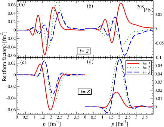
Figure 7: The real parts of the partial wave Coulomb distorted neutron form factors for ²⁰⁸Pb as function of the momentum $p$ for $l=0$ (a) and $l=8$ (c). The form factors are calculated at the first three energies indicated in Table 1 for the given angular momentum, $1\equiv$ 21 MeV, $2\equiv$ 36 MeV, and $3\equiv$ 47 MeV ($l=2$) and 45 MeV ($l=8$). The real parts of the proton form factors for ²⁰⁸Pb as function of the momentum $p$ are given for $l=2$ in (b) and $l=8$ in (d) for the same energies.

In order to illustrate the behavior of Coulomb distorted neutron form factors we show in Fig. 6 in the left panels the real parts of the Coulomb distorted neutron form factors of the $n+^{48}$Ca $t$-matrix for $l=0$ (a) and $l=6$ (c) at the same support points as the plane-wave $n+^{48}$Ca form factors shown in Fig. 3 and the Coulomb distorted $p+^{48}$Ca form factors shown in the right panels. The effect of Coulomb distortions is clearly visible for $l=0$, where the form factor goes to zero as $p\rightarrow 0$. The figure also shows that the Coulomb distorted neutron- and proton form factors are quite different.

In Fig. 7 a similar comparison is shown but for real parts of the Coulomb distorted $n+^{208}$Pb and $p+^{208}$Pb form factors. Drawing attention to the different scales for the left and right side panels, we note that the Coulomb distorted $p+^{208}$Pb form factors do not only differ in shape, but also in magnitude from the Coulomb distorted $n+^{208}$Pb form factors. This may not come as a surprise when having in mind that the Coulomb force is quite strong in heavy nuclei. The comparisons in Figs. 6 and 7 emphasize the need for a proper introduction of the Coulomb force in the EST scheme as presented in Section 3.

The realization that the Coulomb distorted neutron-nucleus form factors differ from the proton-nucleus ones has been already pointed out in Ref. [44] where separable $t$-matrices for proton-proton ($pp$) scattering were considered. There the authors used a separable representation in terms of Yukawa functions and re-adjusted the parameters in the two lowest partial wave to describe the experimentally extracted $pp$ phase shifts. While such an approach may be viable in the $pp$ system, it is not very practical when heavy nuclei are considered, since here many more partial waves are affected by the Coulomb force.

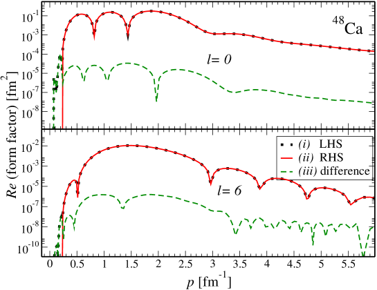
Figure 8: The absolute value of the real part of the partial-wave Coulomb distorted $n+^{48}$Ca for $l=0$ ($E$=6 MeV) and $l=6$ ($E$=16 MeV) as function of the momentum $p$. The dotted lines ($i$) represent the integration over the Coulomb wave functions, while the solid lines ($ii$) stands for the calculations according to right-hand side of Eq. (41). The absolute difference between the two calculation is shown as dashed line ($iii$).

Finally, we want to inspect the Coulomb distorted form factor of Eq. (37) and consider an alternative way for its calculation in order to verify the quite involved integration procedure outlined in this Section and given in detail in Ref. [17]. The quantity $u|f_{l,k_{E}}\rangle$ satisfies an operator LS equation,

$$u|f_{l,k_{E}}\rangle=u|k_{E}\rangle+ug_{0}(E)u|f_{l,k_{E}}\rangle,$$ (40)

where $|k_{E}\rangle$ is the radial part of the solution of the free Hamiltonian at energy $E$ with angular momentum $l$, and $g_{0}(E)$ is the free Green’s function. Multiplying from the left with the Coulomb scattering wave function $\psi^{c}_{l,p}$ gives

$$\langle\psi^{c}_{l,p}|u|f_{l,k_{E}}\rangle=\langle\psi^{c}_{l,p}|u|k_{E}\rangle+\int dp^{\prime}p^{\prime 2}\langle\psi^{c}_{l,p}|u|p^{\prime}\rangle\frac{1}{E-E_{p^{\prime}}+i\epsilon}\langle p^{\prime}|u|f_{l,k_{E}}\rangle.$$ (41)

The term $\langle p^{\prime}|u|f_{l,k_{E}}\rangle=t_{l}(p^{\prime},k_{E};E_{k_{E}})$ is the half-shell $t$-matrix at a support point $E_{k_{E}}$ already calculated when obtaining the form factors for the separable representation (see Eq. (36)). It remains to calculate the driving term, which now is given as

$$\langle\Phi_{l,p^{\prime}}^{c}|u|p\rangle = \frac{2}{\pi}\int\limits_{0}^{\infty}\langle\Phi_{l,p^{\prime}}^{c}|r^{\prime}\rangle\;r^{\prime 2}dr^{\prime}\;\langle r^{\prime}|u|r\rangle\;r^{2}dr\;\langle r|p\rangle$$ (42)

$$= \frac{2}{\pi p^{\prime}}\int\limits_{0}^{\infty}drr^{2}dr^{\prime}r^{\prime}F_{l}(\eta^{\prime},p^{\prime}r^{\prime})\;\langle r^{\prime}|u|r\rangle\;j_{l}(pr),$$ (43)

which turns for the phenomenological Woods-Saxon potential into

$$\langle\Phi_{l,p^{\prime}}^{c}|u|p\rangle=\frac{2}{\pi p^{\prime}}\int\limits_{0}^{\infty}drr\;F_{l}(\eta^{\prime},p^{\prime}r)\;u^{s}(r)\;j_{l}(pr).$$ (44)

We now can evaluate the left-hand side (LHS) and the right-hand side (RHS) of Eq. (41) independently with two completely different algorithms. This comparison is shown for two different form factors for ⁴⁸Ca. For the $l=0$ the form factor at $E$ = 6 MeV is shown, for $l=6$ the one at $E$ = 16 MeV. The results of both independent calculations indistinguishable in the graph. Thus we show the absolute difference between the two calculations as dashed line. This shows that our numerical integration over the momentum-space Coulomb functions together with the Gel’fand-Shilov regularization is very accurate and can be used without any problem in Faddeev-AGS equations formulated in the Coulomb basis when matrix elements in this basis may only be obtained in this fashion.

5 Summary and Outlook

In a series of steps we developed the input that will serve as a basis for Faddeev-AGS three-body calculations of $(d,p)$ reactions, which will not rely on the screening of the Coulomb force. To achieve this, Ref. [6] formulated the Faddeev-AGS equations in the Coulomb basis using separable interactions in the two-body subsystems. For this ambitious program to have a chance of being successful, the interactions in the two-body subsystems, namely the NN and the neutron- and proton-nucleus systems, need to developed so that they separately describe the observables of the subsystems. While for the NN interaction separable representations are available, this is was not the case for the optical potentials describing the nucleon-nucleus interactions. Furthermore, those interactions in the subsystems need to be available in the Coulomb basis.

We developed separable representations of phenomenological optical potentials of Woods-Saxon type for neutrons and protons. First we concentrated on neutron-nucleus optical potentials and generalized the Ernst-Shakin-Thaler (EST) scheme [32] so that it can be applied to complex potentials [15]. In order to consider proton-nucleus optical potentials, we further extended the EST scheme so that it can be applied to the scattering of charged particles with a repulsive Coulomb force [16]. While the extension of the EST scheme to charged particles led to a separable proton-nucleus $t$-matrix in the Coulomb basis, we had to develop methods to reliably compute Coulomb distorted neutron-nucleus $t$-matrix elements [17]. Here we also show explicitly that those calculations can be carried out numerically very accurately by calculating them within two independent schemes.

Our results demonstrate, that our separable representations reproduce standard coordinate space calculations of neutron and proton scattering cross sections very well, and that we are able to accurately compute the integrals leading to the Coulomb distorted form factors. Now that these challenging form factors have been obtained, they can be introduced into the Faddeev-AGS equations to solve the three-body problem without resorting to screening. Our expectation is that solutions to the Faddeev-AGS equations written in the Coulomb-distorted basis can be obtained for a large variety of $n+p+A$ systems, without a limitation on the charge of the target. From those solutions, observables for $(d,p)$ transfer reactions should be readily calculated. Work along these lines is in progress.

Acknowledgments

This material is based on work in part supported by the U. S. Department of Energy, Office of Science of Nuclear Physics under program No. DE-SC0004084 and DE-SC0004087 (TORUS Collaboration), under contracts DE-FG52-08NA28552 with Michigan State University, DE-FG02-93ER40756 with Ohio University; by Lawrence Livermore National Laboratory under Contract DE-AC52-07NA27344 and the U.T. Battelle LLC Contract DE-AC0500OR22725. F.M. Nunes acknowledges support from the National Science Foundation under grant PHY-0800026. This research used resources of the National Energy Research Scientific Computing Center, which is supported by the Office of Science of the U.S. Department of Energy under Contract No. DE-AC02-05CH11231.

References

- [1] J. E. Escher et al., Rev. Mod. Phys. 84, 353 (2012).
- [2] J. Cizewski et al., J. Phys. Conf 420, 012058 (2013).
- [3] R. Kozub et al., Phys.Rev.Lett. 109, 172501 (2012).
- [4] F. Nunes and A. Deltuva, Phys.Rev. C84, 034607 (2011).
- [5] K. Schmitt et al., Phys.Rev.Lett. 108, 192701 (2012).
- [6] A. Mukhamedzhanov, V. Eremenko, and A. Sattarov, Phys.Rev. C86, 034001 (2012).
- [7] A. Deltuva, Phys.Rev. C88, 011601 (2013).
- [8] A. Deltuva, A. Moro, E. Cravo, F. Nunes, and A. Fonseca, Phys.Rev. C76, 064602 (2007), arXiv:0710.5933.
- [9] N. Upadhyay, A. Deltuva, and F. Nunes, Phys.Rev. C85, 054621 (2012), arXiv:1112.5338.
- [10] A. Deltuva and A. Fonseca, Phys.Rev. C79, 014606 (2009).
- [11] E. Alt, P. Grassberger, and W. Sandhas, Nucl. Phys. B 2, 167 (1967).
- [12] A. Deltuva, A. Fonseca, and P. Sauer, Phys.Rev. C71, 054005 (2005).
- [13] A. Deltuva, A. Fonseca, and P. Sauer, Phys.Rev. C72, 054004 (2005).
- [14] F. Nunes and N. Upadhyay, J. Phys. G: Conf. Ser. 403, 012029 (2012).
- [15] The TORUS Collaboration, L. Hlophe et al., Phys.Rev. C88, 064608 (2013).
- [16] L. Hlophe et al., (2014), arXiv:1409.4012.
- [17] TORUS Collaboration, N. Upadhyay et al., Phys. Rev. C90, 014615 (2014).
- [18] J. Haidenbauer and W. Plessas, Phys.Rev. C27, 63 (1983).
- [19] J. Haidenbauer, Y. Koike, and W. Plessas, Phys.Rev. C33, 439 (1986).
- [20] G. Berthold, A. Stadler, and H. Zankel, Phys.Rev. C41, 1365 (1990).
- [21] W. Schnizer and W. Plessas, Phys.Rev. C41, 1095 (1990).
- [22] D. Entem, F. Fernandez, and A. Valcarce, J.Phys. G27, 1537 (2001).
- [23] T. Ueda and Y. Ikegami, Prog.Theor.Phys. 91, 85 (1994).
- [24] A. Gal and H. Garcilazo, Nucl.Phys. A864, 153 (2011).
- [25] A. Ghovanlou and D. R. Lehman, Phys. Rev. C9, 1730 (1974).
- [26] A. Eskandarian and I. R. Afnan, Phys. Rev. C46, 2344 (1992).
- [27] K. Miyagawa and Y. Koike, Prog. Theor. Phys. 82, 329 (1989).
- [28] R. Varner, W. Thompson, T. McAbee, E. Ludwig, and T. Clegg, Phys.Rept. 201, 57 (1991).
- [29] S. Weppner, R. Penney, G. Diffendale, and G. Vittorini, Phys.Rev. C80, 034608 (2009).
- [30] A. Koning and J. Delaroche, Nucl.Phys. A713, 231 (2003).
- [31] J. Becchetti, F.D. and G. Greenlees, Phys.Rev. 182, 1190 (1969).
- [32] D. J. Ernst, C. M. Shakin, and R. M. Thaler, Phys.Rev. C8, 46 (1973).
- [33] D. J. Ernst, J. T. Londergan, E. J. Moniz, and R. M. Thaler, Phys.Rev. C10, 1708 (1974).
- [34] B. Pearce, Phys.Rev. C36, 471 (1987).
- [35] G. Cattapan, G. Pisent, and V. Vanzani, Z.Phys. A274, 139 (1975).
- [36] G. Cattapan, G. Pisent, and V. Vanzani, Nucl. Phys. A241, 204 (1975).
- [37] C. Elster, L. C. Liu, and R. M. Thaler, J.Phys. G19, 2123 (1993).
- [38] C. R. Chinn, C. Elster, and R. M. Thaler, Phys.Rev. C44, 1569 (1991).
- [39] M. Abramovitz and I. Stegun, Handbook of Mathematical FunctionsDover Books on Mathematics (Dover Publications, 1965).
- [40] A. Mukhamedzhanov, private communication (2012).
- [41] E. Dolinskii and A. Mukhamedzhanov, Sov. Jour. Nucl. Phys. 3, 180 (1966).
- [42] The TORUS Collaboration, V. Eremenko et al., to appear in Comp. Phys. Comm. .
- [43] I. Gel’fand and G. Shilov, Generalized Functions, Vol. 1: Properties and Operations. Academic Press (1964).
- [44] W. Schweiger, W. Plessas, L. Kok, and H. van Haeringen, Phys.Rev. C27, 515 (1983).