Abstract

In the first part we present the number theoretical properties of the Riemann zeta function and formulate the Riemann Hypothesis. In the second part we review some physical problems related to this hypothesis: the Polya–Hilbert conjecture, the links with Random Matrix Theory, relation with the Lee–Yang theorem on the zeros of the partition function, random walks, billiards etc.

MSC: 11M01, 11M26, 11M50, 81-02, 82B41

“… upon looking at prime numbers one has the feeling of being
                                       in the presence of one of the inexplicable secrets of creation.”
                                                                                      Don Zagier in [1, p.8, left column]

1 Introduction

There are many links between mathematics and physics. Many branches of mathematics arose from the need to formalize and clarify the calculations carried out by physicists, e.g. Hilbert spaces, distribution theory, differential geometry etc. In this article we are going to describe the opposite situation when the famous open mathematical problem can be perhaps solved by physical methods. We mean the Riemann Hypothesis (RH), the over 160 years old problem which solution is of central importance in many branches of mathematics: there are probably thousands of theorems beginning with: “Assume that the Riemann Hypothesis is true, then …”. The RH appeared on the Hilbert’s famous list of problems for the XX centaury as the first part of the eighth problem [2] (second part concerned the Goldbach’s conjecture; recently H. A. Helfgott [3] have solved so called ternary case of Goldbach conjecture). In the year 2000 RH appeared on the list of the Clay Mathematics Institute problems for the third millennium, this time with 1,000,000 US dollars reward for the solution.

After the announcement of the prize by Clay Mathematics Institute for solving RH there has been a rash of popular books devoted to this problem: [4], [5], [6], [7], [8]. The classical monographs on RH are: [9], [10], [11], [12], while [13] is a collection of original papers devoted to RH preceded by extensive introduction to the subject. We also strongly recommend the web site Number Theory and Physics at the address http://empslocal.ex.ac.uk/people/staff/mrwatkin/zeta/physics.htm containing a lot information about links between number theory (in particular about RH) and physics.

In 2011 there appeared the paper “Physics of the Riemann hypothesis” written by D. Schumayer and D. A.W. Hutchinson [14]. Here we aim to provide complementary description of the problem which can serve as a starting point for the interested reader.

This review consists of seven Sections and the Concluding Remarks. In the next Section we present the historical path leading to the formulation of the RH. Next we briefly discuss possible ways of proving the RH. Next two Sections concern connections between RH and quantum mechanics and statistical mechanics. In Sect.6 a few other links between physical problems and RH are presented. In the last Section fractal structure of the Riemann $\zeta(s)$ function is discussed. Because we intend this article to be a guide we enclose rather exhaustive bibliography containing over 100 references, a lot of these papers can be downloaded freely from author’s web pages. Let us begin the story.

2 The short history of the Prime Number Theorem

There are infinitely many prime numbers $2,3,5,7,11,\ldots,p_{n},\ldots$ and the first proof of this fact was given by Euclid in his Elements around 330 years b.C. His proof was by contradiction: Assume there is a finite set of primes $\mathcal{P}=\{2,3,5,\ldots,p_{n}\}$. Form the number $2\times 3\times 5\ldots\times p_{n}+1$, then this number divided by primes from $\mathcal{P}$ gives the remainder 1, thus it has to be a new prime or it has to factorize into primes not contained in the set $\mathcal{P}$, hence there must be more primes than $n$. For example if $\mathcal{P}=\{2,3,5,7,11,13\}$, then $2\cdot 3\cdot 5\cdot 7\cdot 11\cdot 13+1=59\cdot 509$ and $59,509\notin\mathcal{P}$. The first direct proof of infinity of primes was presented by L. Euler around 1740 who has shown that the harmonic sum of prime numbers $p_{n}$ diverges:

$$\sum_{p_{n}<x}~{}\frac{1}{p_{n}}\sim\log\log(x).$$

Next the problem of determining the function $\pi(x)=\sum_{n}\Theta(x-p_{n})$ ($\Theta(x)$ is the Heaviside step function), giving the number of primes up to a given threshold $x$, has arisen. It is one of the greatest surprises in the whole mathematics that such an erratic function as $\pi(x)$ can be approximated by a simple expression. Namely Carl Friedrich Gauss as a teenager (different sources put his age between fifteen years and seventeen years) has made in the end of eighteen centaury the conjecture that $\pi(x)$ is very well approximated by the logarithmic integral $\rm{Li}(x)$:

$$\pi(x)\sim{\rm{Li}}(x):=\int_{2}^{x}\frac{du}{{\log(u)}}.$$ (1)

The symbol $f(x)\sim g(x)$ means here that $\lim_{x\rightarrow\infty}f(x)/g(x)=1$. Integration by parts gives the asymptotic expansion which should be cut at the term $n_{0}=\lfloor\log(x)\rfloor$, after which terms begin to increase:

$${\rm Li}(x)=\frac{x}{\log(x)}+\frac{x}{\log^{2}(x)}+\frac{2!x}{\log^{3}(x)}+\frac{3!x}{\log^{4}(x)}+\cdots.$$ (2)

There is a series giving $\rm{Li}(x)$ for all $x>2$ and quickly convergent which has $n!$ in denominator and $\log^{n}(x)$ in nominator instead of opposite order in (2) (see [15, Sect. 5.1])

$${\rm{Li}}(x)=\gamma+\log\log(x)+\sum_{n=1}^{\infty}\frac{\log^{n}(x)}{n\cdot n!}\quad{\rm for}~{}x>1~{},$$ (3)

where $\gamma\approx 0.577216$ is the Euler- Mascheroni constant $\gamma=\lim_{n\rightarrow\infty}\left(\sum_{k=1}^{n}\frac{1}{k}-\log(n)\right)$.

The way of proving (1) was outlined by Bernhard Riemann in a seminal 8-pages long paper published in 1859 [16]. English translation is available at http://www.maths.tcd.ie/pub/HistMath/People/Riemann or at CMI web page; it was also included as an appendix in [10]. The handwritten by Riemann manuscript was saved by his wife and is kept in the Manuscript Department of the Niedersöchsische Staats und Universitätsbibliothek Göttingen. The scanned pages are available at http://www.claymath.org/sites/default/files/riemann1859.pdf. In fact in this paper Riemann has given an exact formula for $\pi(x)$. The starting point of the Riemann’s reasoning was the mysterious formula discovered by Euler linking the sum of $\frac{1}{n^{ks}}$ with the product over all primes $p$:

$$\zeta(s):=\sum_{n=1}^{\infty}\frac{1}{n^{s}}=\prod_{p=2}^{\infty}\frac{1}{\left(1-\frac{1}{p^{s}}\right)},~{}~{}~{}~{}s=\sigma+it,~{}~{}~{}~{}\Re[s]=\sigma>1.$$ (4)

To see that this equality really holds one needs first to recognize in the terms $1/{\left(1-\frac{1}{p^{s}}\right)}$ the sums of the geometric series $\sum_{k=0}^{\infty}\frac{1}{p^{s}}$. The geometrical series converges absolutely so the interchange of summation and the product is justified. Finally the fundamental theorem of arithmetic stating the each positive integer $n>1$ can be represented in exactly one way (up to the order of the factors) as a product of prime powers:

$$n=p_{1}^{\alpha_{1}}p_{2}^{\alpha_{2}}\cdots p_{k}^{\alpha_{k}}=\prod_{i=1}^{k}p_{i}^{\alpha_{i}}.$$ (5)

has to be invoking to obtain the series on lhs of (4). Let us notice that on the rhs (4) the product cannot start from $p=1$ and it explains why the first prime is 2 and not 1 — physicists often think that 1 is a prime number (before 19–th century $1$ was indeed considered to be a prime). Euler was the first who calculated the sums $\sum_{n=1}^{\infty}\frac{1}{n^{2}}=\pi^{2}/6,~{}\sum_{n=1}^{\infty}\frac{1}{n^{4}}=\pi^{4}/90$ and in general $\zeta(2n)$. In fact Euler has considered the above formula only for real exponents $s=x$ and it was Riemann who considered it as a function of complex argument $s=\sigma+it$ and thus the function $\zeta(s)$ is called the Riemann’s zeta function. In the context of RH instead of $z=x+iy$ for the complex variable the notation $s=\sigma+it$ is traditionally used. The formula (4) is valid only for $\Re[s]=\sigma>1$ and it follows from the product of non-zero terms on r.h.s. of (4) that $\zeta(s)\neq 0$ on the right of the line $\Re[s]=1$. Riemann has generalized $\zeta(s)$ to the whole complex plane without $s=1$ where zeta is divergent as an usual harmonic series — the fact established in 14th century by Nicole Oresme. Riemann did it by analytical continuation (for the proof see the original Riemann’s paper or e.g. [10, Sect. 1.4]:

$$\zeta(s)=\frac{\Gamma(-s)}{2\pi i}\int_{+\infty}^{+\infty}\frac{(-x)^{s}}{e^{x}-1}\frac{dx}{x},$$ (6)

where $\int_{+\infty}^{+\infty}$ denotes the integral over the contour

Appearing in (6) the gamma function $\Gamma(z)$ has many representations, we present the Weierstrass product:

$$\Gamma(z)=\frac{e^{-\gamma z}}{z}\prod_{k=1}^{\infty}\left(1+\frac{z}{k}\right)^{-1}e^{z/k}\,.$$ (7)

From (7) it is seen that $\Gamma(z)$ is defined for all complex numbers $z$, except $z=-n$ for integers $n>0$, where are the simple poles of $\Gamma(z)$. The most popular definition of gamma function given by the integral $\Gamma(z)=\int_{0}^{\infty}e^{-t}t^{z-1}dt$ is valid only for $\Re[z]>0$.

The integral (6) is well defined on the whole complex plane without $s=1$, where $\zeta(s)$ has the simple pole, and is equal to (4) on the right of the line $\Re[s]=1$. Recently many representations of the $\zeta(s)$ are known, for review of the integral representations see [17].

The exact formula for $\pi(x)$ obtained by Riemann involves the function $J(x)$ defined as

$$J(x)=\pi(x)+\frac{1}{2}\pi(x^{1/2})+\frac{1}{3}\pi(x^{1/3})+\cdots.$$ (8)

In words $J(x)$ increases by 1 at each prime number $p$, by $1/2$ at each $x$ being the square of the prime, in general it jumps by $1/n$ at argument equal to $n$-th power of some prime $p^{n}$. $J(x)$ is discontinuous at $x=p^{n}$ thus at such arguments is defined as a halfway between its old value and its new value. Let us mention that $J(x)=0$ for $0\leq x<2$. Then $\pi(x)$ is given (via so called Möbius inversion formula) by the series:

$$\pi(x)=\sum_{n\geq 1}\frac{\mu(n)}{n}J(x^{1/n}),$$ (9)

where the sum is in fact finite because it stops at such $N$ that $x^{1/N}>2>x^{1/(N+1)}$ and $\mu(n)$ is the Möbius function:

$$\mu(n)\,=\,\left\{\begin{array}[]{ll}1&\mbox{for}~{}~{}n=1\\ 0&\mbox{when {\it n} is divisible by the square of some prime {\it p}:}~{}~{}p^{2}|n\\ (-1)^{r}&\mbox{ when }~{}n=p_{1}p_{2}\ldots p_{r}\end{array}\right.$$ (10)

For example $\mu(14)=1,\mu(25)=0,\mu(30)=-1$. This definition of $\mu(n)$ stems from the formula (4) and the Dirichlet series for the reciprocal of the zeta function:

$$\frac{1}{\zeta(s)}=\prod_{p=2}^{\infty}\left(1-\frac{1}{p^{s}}\right)=\sum_{n=1}^{\infty}\frac{\mu(n)}{n^{s}}.$$ (11)

The above product over $p$ produces integers $n$ which in the factorization does not contain square of a prime and those $n$ which factorizes into odd number of primes contribute with sign $-1$ while those $n$ which factorizes into even number of primes contribute with sign $+1$. We can notice at this point that the Möbius function has the physical interpretation: namely in [18] it was shown that $\mu(n)$ can be interpreted as the operator $(-1)^{F}$ giving the number of fermions in quantum field theory. In this approach the equality $\mu(n)=0$ for $n$ divisible by a square of some prime is the manifestation of the Pauli exclusion principle.

The crucial point of the Riemann’s reasoning was the alternative formula for $J(x)$ not involving primes at all:

$$J(x)={\rm{Li}}(x)-\sum_{\rho}{\rm{Li}}(x^{\rho}),$$ (12)

where the sum runs over all zeros of $\zeta(s)$, i.e. over such $\rho$ that $\zeta(\rho)=0$. Let us stress that the above (12) is an equality, which is remarkable because the left hand side is a step function, thus somehow at prime powers all of the zeros of zeta cooperate to deform smooth plot of the first term ${\rm{Li}}(x)$ into the stair–like graph with jumps. Then the number of primes up to $x$ is obtained by combining (9) and (12)

$$\pi(x)=\sum_{n=1}^{N}\frac{\mu(n)}{n}\left({\rm{Li}}(x^{1/n})-\sum_{\rho}{\rm{Li}}(x^{\rho/n})\right).$$ (13)

To be precise at arguments $x$ equal to prime numbers, when $\pi(x)$ is not continuous and jumps by 1, one has to define lhs as $\lim_{\epsilon\rightarrow\infty}\{\pi(x-\epsilon)+\pi(x+\epsilon)\}$ (the same procedure was mentioned above for the function $J(x)$). There is an ambiguity when using definition of logarithmic integral (1) for ${\rm{Li}}(x^{\rho})$ connected with multivaluedness of logarithm of complex argument, in particular for complex numbers $z_{1},z_{2}$ the equality $\log(z_{1}z_{2})=\log(z_{1})+\log(z_{2})$ does not hold (here are calculations providing the counterexample: $(-z)^{2}=z^{2},~{}\log((-z)^{2})=\log(z^{2}),~{}\log(-z)+\log(-z)=\log(z)+\log(z),~{}2\log(-z)=2\log(z)\Rightarrow\log(-z)=\log(z)$; in particular $\log(-1)=\log(1)=0$ what is not true as $\log(-1)=i(2k+1)\pi\neq 0$). Hence the above logarithmic integral for complex argument is defined as ${\rm{Li}}(x^{\rho})={\rm{Li}}(e^{\rho\log(x)})$, where for $z=u+iv,~{}v\neq 0$:

$${\rm{Li}}(e^{z})=\int_{-\infty+iv}^{u+iv\\ ~{}~{}~{}~{}}\frac{e^{w}}{w}dw,$$ (14)

thus $\rm{Li}$ is in fact defined via the exponential integral. Let us mention, that in Mathematica to obtain the value of ${\rm{Li}}(x^{\rho_{k}})$ the command ExpIntegralEi[ZetaZero[k]*Log[x]] has to be used.

In equations (12) and (13) we meet the issue of determining zeros $\rho$ of the zeta function: $\zeta(\rho)=0$. Riemann has shown that $\zeta(s)$ fulfills the functional identity:

$$\pi^{-\frac{s}{2}}\Gamma\left(\frac{s}{2}\right)\zeta(s)=\pi^{-\frac{1-s}{2}}\Gamma\left(\frac{1-s}{2}\right)\zeta(1-s),~{}~{}~{}~{}{\rm for}~{}s\in\mathbb{C}\setminus\{0,1\}.$$ (15)

The above form of the functional equation is explicitly symmetrical with respect to the line $\Re(s)=1/2$: the change $s\rightarrow\frac{1}{2}+s$ on both sides of (15) shows that the values of the combination of functions $\pi^{-\frac{s}{2}}\Gamma\left(\frac{s}{2}\right)\zeta(s)$ are the same at points $\frac{1}{2}+s$ and $\frac{1}{2}-s$.

Because $\Gamma(z)$ is singular at all negative integers, thus to fulfill functional identity (15) $\zeta(s)$ has to be zero at all negative even integers:

$$\zeta(-2n)=0,n=1,2,3,\ldots$$

These zeros are called trivial zeros. The fact that $\zeta(s)\neq 0$ for $\Re(s)>1$ and the shape of the functional identity entails that nontrivial zeros $\rho_{n}=\beta_{n}+i\gamma_{n}$ are located in the critical strip:

$$0\leq\Re[\rho_{n}]=\beta_{n}\leq 1.$$

From the symmetry of the functional equation (15) with respect to the line $\Re[s]=\frac{1}{2}$ it follows, that if $\rho_{n}=\beta_{n}+i\gamma_{n}$ is a zero, then $\overline{\rho_{n}}=\beta_{n}-i\gamma_{n}$ and $1-\rho_{n},~{}1-\overline{\rho_{n}}$ are also zeros: they are located symmetrically around the straight line $\Re[s]=\frac{1}{2}$ and the axis $t=0$, see Fig. 1.

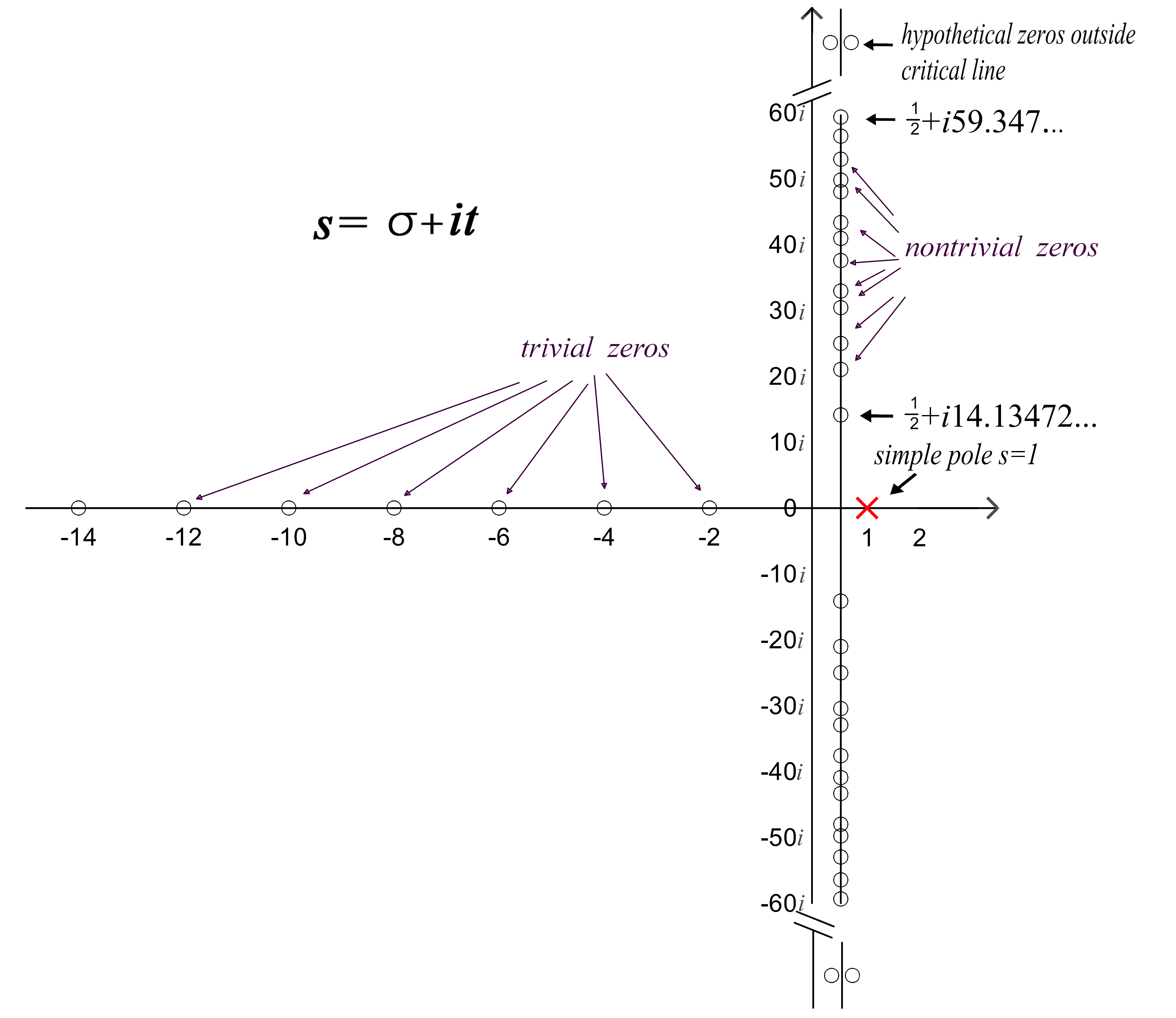
Figure 1: The location of zeros of the Riemann $\zeta(s)$ function.

The sum over trivial zeros $\rho=-2n$ in (12) can be calculated analytically giving the explicit (i.e. expressed directly by sum over zeros of $\zeta(s)$) formula for $J(x)$:

$$J(x)={\rm{Li}}(x)-\sum_{\begin{subarray}{c}\Re(\rho)>0\\ 0<\Im(\rho)<1\end{subarray}}\left({\rm{Li}}(x^{\rho})+{\rm{Li}}(x^{\overline{\rho}})\right)+\int_{x}^{\infty}\frac{du}{u(u^{2}-1)\log(t)}-\log(2)$$ (16)

and therefore explicit formula for $\pi(x)$ follows:

$$\pi(x)=\sum_{n=1}^{N}\frac{\mu(n)}{n}\left({\rm{Li}}(x^{\frac{1}{n}})-\sum_{\begin{subarray}{c}\Re(\rho)>0\\ 0<\Im(\rho)<1\end{subarray}}\Bigl{(}{\rm{Li}}(x^{\frac{\rho}{n}})+{\rm{Li}}(x^{\frac{\overline{\rho}}{n}})\Bigr{)}+\int_{x^{1/n}}^{\infty}\frac{1}{u\left(u^{2}-1\right)\log(u)}\,du-\log(2)\right).$$ (17)

Extending in the first term summation to infinity (it is not an big sin, as terms with large $n$ tend to zero) gives the function

$$R(x)=\sum_{n=1}^{\infty}\frac{\mu(n)}{n}{\rm Li}(x^{1/n}).$$ (18)

The function $R(x)$ can be calculated from very quickly converging series

$$R(x)=1+\sum_{n=1}^{\infty}\frac{\left(\log(x)\right)^{n}}{nn!\zeta(n+1)}.$$ (19)

The last sum is called the Gram formula, see [19, p.51] for transformations leading from (18) to (19). Because the sum over all complex zeros is not absolutely convergent its value depends on the order of summation. In fact famous (and curious) Riemann’s rearrangement theorem, see e.g. [20, Theorem 3.54], asserts that terms of a conditionally convergent infinite series can be permuted such a way that the new series converges to any given value ! For (17) Riemann in [16] says that “It may easily be shown, by means of a more thorough discussion” that the natural order , i.e. the process of pairing together zeros $\rho$ and $\overline{\rho}$ in order of increasing imaginary parts of $\rho$, is the correct one. At the end of [16] Riemann states about the series in (17) that “when reordered it can take on any arbitrary real value”.

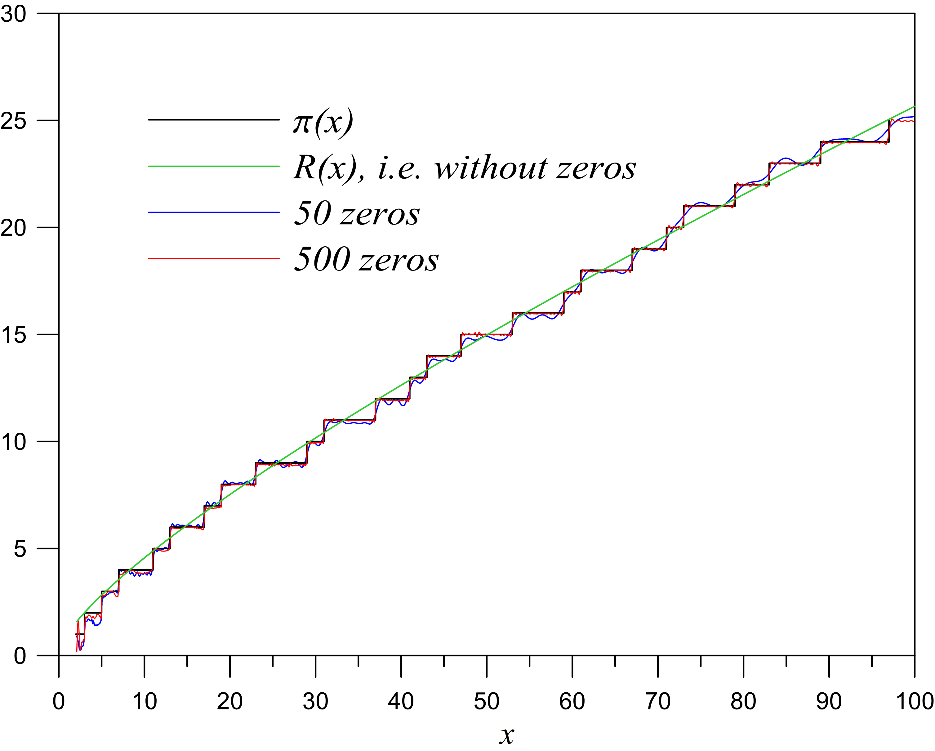
Figure 2: The plot of $\pi(x)$ and the r.h.s. of (17) obtained by summing over first 50 nontrivial zeros (blue line) and first 500 nontrivial zeros (red line). We have produced data for this plots using the equation (22). The animation showing the effect of adding consecutive zeros one by one to the formula (17) can be seen at http://empslocal.ex.ac.uk/people/staff/mrwatkin/zeta/encoding1.htm

Again let us point out the curiosity (mystery) of the above equation (17): $\pi(x)$ on lhs jumps by 1 at each argument being a prime with constant values (horizontal sections) between two consecutive primes. Thus on the rhs the zeros of zeta have to conspire to deform smooth plot of the first term ${\rm{Li}}(x)$ into the stair–like graph with jumps. It resembles the Fourier series of smooth sinuses reproducing say the step function on interval $(-\pi,\pi)$. In Fig. 2 we have made plots illustrating these observations.

The formula (17) is less time consuming to obtain $\pi(x)$ for large $x$ than counting all primes up to $x$; the best non–analytical methods of computing $\pi(x)$ have complexity $\mathcal{O}(x^{2/3}/\log^{2}(x))$, while involving some variants of the Riemann explicite formula are $\mathcal{O}(x^{1/2})$ in time. For example, the value $\pi(10^{24})=18,435,599,767,349,200,867,866$ was obtained by a variant of (17) using $59,778,732,700$ nontrivial zeros of $\zeta(s)$ [21]. Also the value $\pi(10^{25})=176,846,309,399,143,769,411,680$ was announced, see The On-Line Encyclopedia of Integer Sequence, entry A006880.

Amazingly the horrible looking sum of the integrals in (17) stemming from the trivial zeros can be brought to the simple closed form:

$$\sum_{n=1}^{N}\frac{\mu(n)}{n}\left(\int_{x^{1/n}}^{\infty}\frac{1}{u\left(u^{2}-1\right)\log(u)}\,du-\log(2)\right)=\frac{1}{2\log x}\sum_{n=1}^{N}\mu(n)+\frac{1}{\pi}\arctan\frac{\pi}{\log x}+\epsilon(x,N),$$ (20)

where $\epsilon(x,N)\rightarrow 0$ as $N\rightarrow\infty$, for details see [22]. The special choice of $N$ such that $\sum_{k=1}^{N}\mu(k)=-2$ (e.g. $N=5,7,8,9,11,12,\ldots$) is favoured: the series for arcus tangens in the vicinity of $u=0$ has the form $\arctan(u)=u-u^{3}/3+u^{5}/5-u^{7}/7+\ldots$ and for such a special $N$ the first two terms in (20) behave together like $(\pi/\log(x))^{3}/3+\ldots$ thus the contribution from trivial zeros is negligible for large $x$ and hence nontrivial zeros are prevailing.

So where are the complex zeros of zeta? Riemann has made the assumption, now called the Riemann Hypothesis, that all nontrivial zeros lie on the critical line $\Re[s]=\frac{1}{2}$:

$$\rho_{n}=\frac{1}{2}+i\gamma_{n}~{}~{}~{}~{}~{}(\mbox{i.e. }~{}~{}\beta_{n}=\frac{1}{2}~{}~{}\mbox{for all}~{}~{}n).$$ (21)

Contemporary the above requirement is augmented by the demand that all nontrivial zeros are simple. Despite many efforts the Riemann Hypothesis remains unproved. In Fig.1 we illustrate the Riemann Hypothesis and in the Table 1 we give the approximate values of the first 10 non-trivial zeros of $\zeta(s)$. We see that initially $\gamma_{n}>n$, but at $n=9137$ the inequality reverses as $\gamma_{9137}=9136.6792\ldots$ while $\gamma_{9136}=9136.1396\ldots$. Next zero is again larger than its index: $\gamma_{9138}=9138.10591\ldots$ but $\gamma_{9141}=9140.5783\ldots$ and up to $n=10,000,000$ the inequality $\gamma_{n}<n$ holds and we believe it will be fulfilled for ever. Incidentally $9137$ is a prime, in fact it is a left–truncatable prime: removing successively left digit gives again prime numbers 9137, 137, 37 and 7.

Table 1

$n$	$\tfrac{1}{2}+i\gamma_{n}$	$n$	$\tfrac{1}{2}+i\gamma_{n}$
$~{}~{}1~{}~{}~{}$	${\tfrac{1}{2}}+i14.134725142\ldots~{}$	$~{}~{}6~{}~{}~{}$	${\tfrac{1}{2}}+i37.586178159\ldots~{}$
$~{}~{}2~{}~{}~{}$	${\tfrac{1}{2}}+i21.022039639\ldots~{}$	$~{}~{}7~{}~{}~{}$	${\tfrac{1}{2}}+i40.918719012\ldots~{}$
$~{}~{}3~{}~{}~{}$	${\tfrac{1}{2}}+i25.010857580\ldots~{}$	$~{}~{}8~{}~{}~{}$	${\tfrac{1}{2}}+i43.327073281\ldots~{}$
$~{}~{}4~{}~{}~{}$	${\tfrac{1}{2}}+i30.424876126\ldots~{}$	$~{}~{}9~{}~{}~{}$	${\tfrac{1}{2}}+i48.005150881\ldots~{}$
$~{}~{}5~{}~{}~{}$	${\tfrac{1}{2}}+i32.935061588\ldots~{}$	$~{}~{}10~{}~{}~{}$	${\tfrac{1}{2}}+i49.773832478\ldots~{}$

Assuming the RH, i.e. collecting together terms $\rho_{n}=\frac{1}{2}+i\gamma_{n}$ and $\overline{\rho_{n}}=1-\rho_{n}=\frac{1}{2}-i\gamma_{n}$, using the Euler identity $e^{i\alpha}=\cos(\alpha)+i\sin(\alpha)$ we can represent $\pi(x)$ as a main smooth trend plus superposition of waves $\sin(\cdot)$ and $\cos(\cdot)$:

$$\begin{split}\pi(x)=1+\sum_{n=1}^{\infty}\frac{(\log(x))^{n}}{nn!\zeta(n+1)}~{}-~{}~{}~{}~{}~{}~{}~{}~{}~{}~{}~{}~{}~{}~{}~{}~{}~{}~{}~{}~{}\\ \sum_{n}\mu(n)\frac{x^{\frac{1}{2n}}}{\log(x)}\sum_{i}\Biggl{\{}\frac{\cos\left(\frac{\gamma_{i}\log(x)}{n}\right)+2\gamma_{i}\sin\left(\frac{\gamma_{i}\log(x)}{n}\right)}{\frac{1}{4}+\gamma_{i}^{2}}\\ +\frac{n}{\log(x)}\frac{(\frac{1}{4}-\gamma_{i}^{2})2\cos\left(\frac{\gamma_{i}\log(x)}{n}\right)+2\gamma_{i}\sin\left(\frac{\gamma_{i}\log(x)}{n}\right)}{\frac{1}{16}+\frac{1}{2}\gamma_{i}^{2}+\gamma_{i}^{4}}\Biggr{\}},\\ \end{split}$$ (22)

where we have used two first terms of the expansion ${\rm{Li}}(x)\approx x/\log(x)+x/\log^{2}(x)$. Using the above equation with 10000 zeros and second sum over $n$ up to 7 we obtained $25.00267$ for $\pi(100)$, while the numbers of primes up to 100 (without counting 1 as a prime) is 25. Physicists well know that derivative of the step function is the Dirac delta function: $\Theta^{\prime}(x)=\delta(x)$, thus the derivative of $\pi(x)$ with respect to $x$ is the sum of Dirac deltas concentrated on primes: $\sum_{p_{n}}\delta(x-p_{n})$. We have differentiated two first sums in (22), i.e. skipping terms $\mathcal{O}(1/\gamma_{k}^{4})$, summed over first 15000 nontrivial zeros of zeta and the resulting plot is presented in Fig.3. The animated plot of the delta–like spikes emerging with increasing number of nontrivial zeros taken into account is available at http://empslocal.ex.ac.uk/people/staff/mrwatkin/zeta/pianim.htm.

In 1896 J. S. Hadamard (1865 – 1963) and Ch. J. de la Vall e Poussin (1866 – 1962) independently proved that $\zeta(s)$ does not have zeros on the line $1+it$, thus $|x^{\rho}|<x$. It suffices to obtain from (17) the original Gauss’s guess (1), which thus became a theorem called the Prime Number Theorem (PNT). Indeed: for large $x$ in (17) the first term $R(x)$ wins over terms with ${\rm{Li}}(x^{\rho})$ and then from (18) we have that $R(x)\approx{\rm{Li}}(x)$.

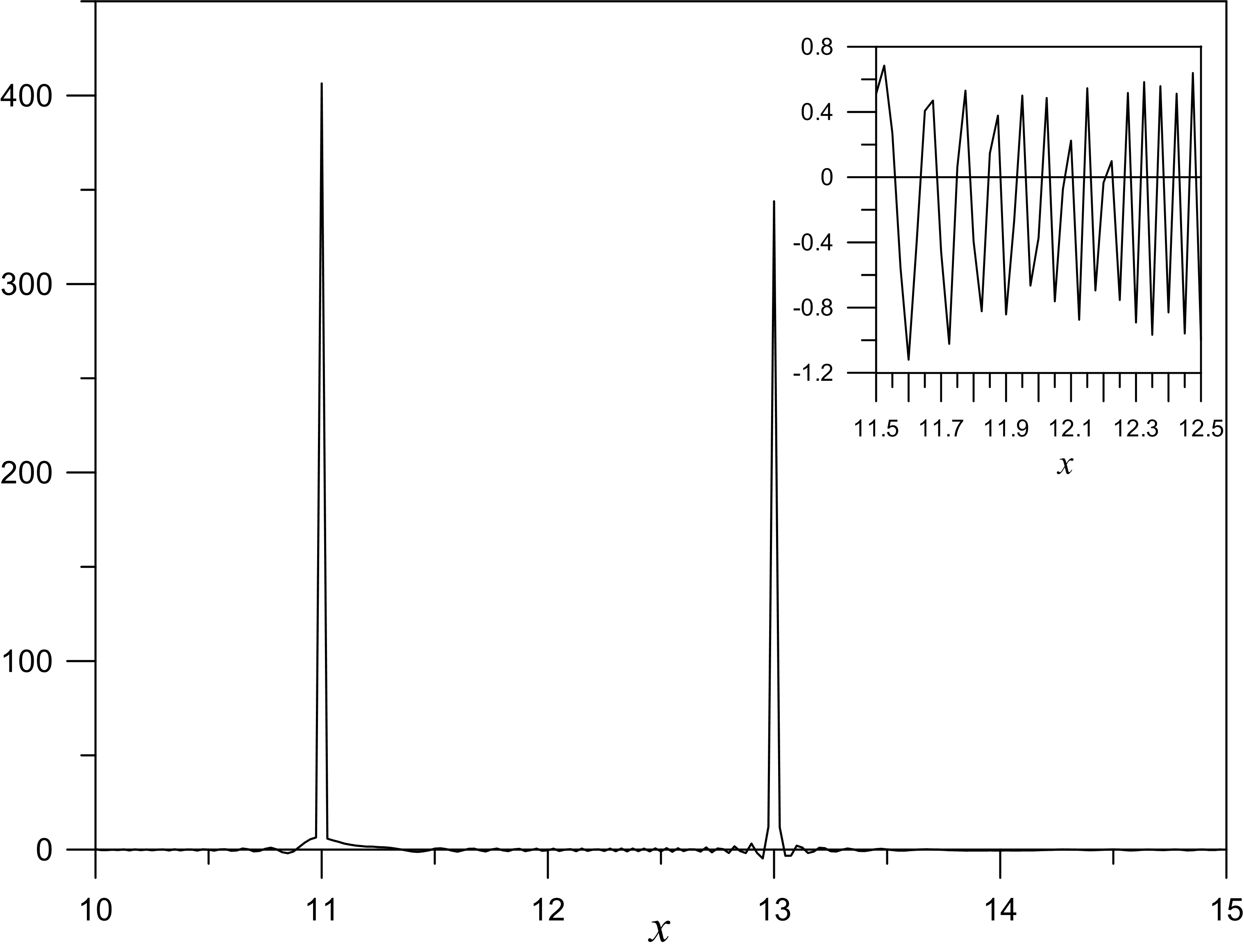
Figure 3: The plot of the derivative of two sums on rhs of (22) obtained by summing over first 15000 nontrivial zeros showing delta–like pattern. In the inset fluctuations for $11.5<x<12.5$ are shown — the high spikes at $x=11$ and $13$ squeezed them on the original plot.

Already Riemann calculated numerically a few first nontrivial zeros of $\zeta(s)$ [10]. Next in 1903 J.P. Gram [23] calculated that first 15 zeros of $\zeta(s)$ are on the critical line; in June of 1950 A.Turing has used the Mark 1 Electronic Computer at Manchester University to check that first 1104 zeros are on the critical line. He has done this calculations “in an optimistic hope that a zero would be found off critical line”, see [24, p. 99]. A few years ago S. Wedeniwski (2005) was leading the internet project Zetagrid [25] which during four years determined that $250\times 10^{12}$ zeros are on the critical line, i.e. on $s=\frac{1}{2}+it$ up to $~{}t<29,538,618,432.236$. The present record belongs to K. Gourdon(2004) [26]: the first $10^{13}$ zeros are on the critical line. A. Odlyzko checked that RH is true in different intervals around $10^{20}$ [27], $10^{21}$ [28], $10^{22}$ [29], but his aim was not to verify the RH but rather providing evidence for conjectures that relate nontrivial zeros of $\zeta(s)$ to eigenvalues of random matrices, see Sect. 4. In fact Odlyzko has expressed the view that the hypothetical zeros off the critical line are unlikely to be encountered for $t$ below $10^{10^{10000}}$, see [4, p.358].

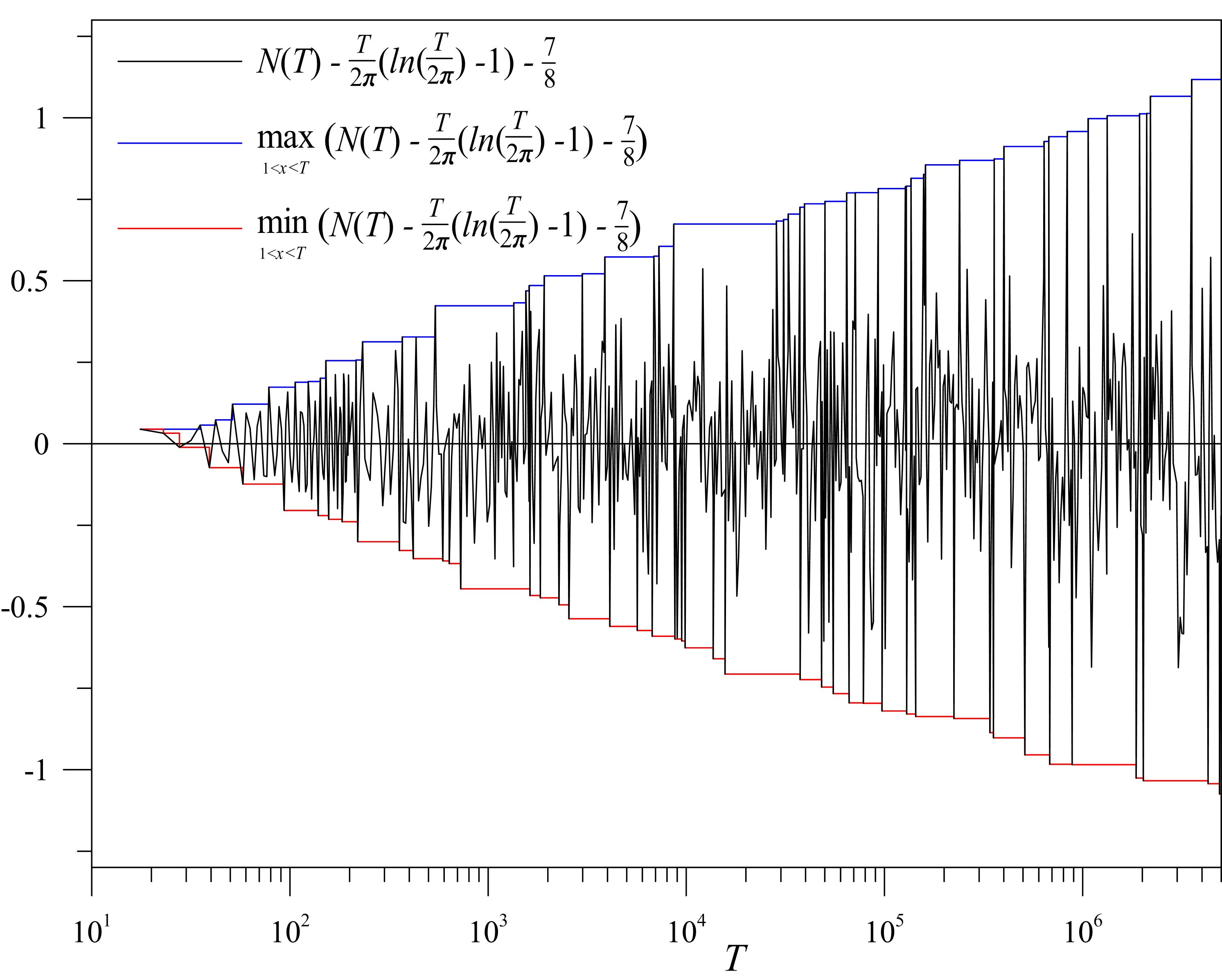
Figure 4: The plot illustrating the formula (23) for number of nontrivial zeros up to $T=5\times 10^{6}$. When on vertical axis the interval (0,1) is 4 cm long, then if the horizontal axis would be plotted on linear scale instead of logarithmic, its length should amount to 200 km. This analogy in a striking way shows how precise is the formula (23) and that the term $7/8$ is important (mathematicians will not agree with this and skip this constant term).

Let $N(t)$ denote the function counting the nontrivial zeros up to $T$, i.e. $N(T)=\sum_{n}\Theta(T-\Im[\rho_{n}])$. In his seminal paper Riemann announced and in 1905 von Mangoldt proved that:

$$N(T)=\frac{T}{2\pi}\log\left(\frac{T}{2\pi e}\right)+\frac{7}{8}+{\mathcal{O}}(\log(T)).$$ (23)

The Fig.4 illustrates how well the above formula predicts $N(T)$. In 1904 G.H. Hardy proved, by considering moments of certain functions related to the zeta function, that on the critical line there is infinity of zeros of $\zeta(s)$ [30]. Levinson (1974) proved that more than one-third of zeros of Riemann s $\zeta(s)$ are on critical line by relating the zeros of the zeta function to those of its derivative, and Conrey (1989) improved this further to two-fifths (precisley 40.77 % have $\Re(\rho)=\tfrac{1}{2}$). The present record seems to belong to S. Feng, who proved that at least 41.28% of the zeros of the Riemann zeta function are on the critical line [31].

At the end of this Section we mention, that $\zeta(s)$ admits besides the product (4) another product representation, called the Hadamard product:

$$\zeta(s)=\frac{\pi}{(s-1)\Gamma\left(\frac{s}{2}-1\right)}e^{-1-\frac{\gamma}{2}}\prod_{k=1}^{\infty}e^{\frac{s}{\rho_{k}}}\left(1-\frac{s}{\rho_{k}}\right).$$ (24)

In contrast to (4) it is valid on the whole complex plane without $s=1$. It is an example of the general Weierstrass factorization theorem: points where function vanishes determine this function. We also add that the common belief is that the imaginary parts $\gamma_{l}$ of the nontrivial zeros of $\zeta(s)$ are irrational and perhaps even transcendental [32], [33].

3 How to prove the Riemann Hypothesis?

Practically nobody is going to prove the RH directly: there are probably well over one hundred of different facts either equivalent to RH or of whose truth RH will follow (i.e. sufficient conditions). Hence proving one of these so called criteria for RH will entail the validity of RH. Below we present a few such criteria for RH.

In 1901 H. von Koch proved [34] that the Riemann Hypothesis is equivalent to the following error term for the approximation of the prime counting function by logarithmic integral:

$$\pi(x)={\rm Li}(x)+{\mathcal{O}}(\sqrt{x}\log(x)).$$ (25)

Later the error term was specified explicitly by Schoenfeld [35, Corollary 1] and RH is equivalent to

$$|\pi(x)-{\rm Li}(x)|\leq\frac{1}{8\pi}\sqrt{x}\log(x)\mbox{ for all }x\geq 2657.$$ (26)

The following facts show that the validity of the RH is very delicate and subtle: namely in some sense RH is valid with accuracy $\epsilon=1.14541\times 10^{-11}$ (or less, that is the present value of $\epsilon$). Here is the reasoning leading to this conclusion: Let us introduce the function

$$\xi(iz)=\frac{1}{2}\left(z^{2}-\frac{1}{4}\right)\pi^{-\frac{z}{2}-\frac{1}{4}}\Gamma\left(\frac{z}{2}+\frac{1}{4}\right)\zeta\left(z+\frac{1}{2}\right).$$ (27)

We can see from the above formula that: RH is true $\Leftrightarrow$ all zeros of $\xi(iz)$ are real. The point is that $\xi(z)$ can be expressed as the following Fourier transform (for derivation of this formula see e.g. [9, Sect.10.1]):

$$\frac{1}{8}\xi\left(\frac{z}{2}\right)=\int_{0}^{\infty}\Phi(t)\cos(zt)dt,$$ (28)

where

$$\Phi(t)=\sum_{n=1}^{\infty}(2\pi^{2}n^{4}e^{9t}-3\pi n^{2}e^{5t})e^{-\pi n^{2}e^{4t}}.$$ (29)

The functin $\xi(z)$ can be generalized to the family of functions $H(z,\lambda)$ parameterized by $\lambda$:

$$H(z,\lambda)=\int_{0}^{\infty}\Phi(t)e^{\lambda t^{2}}\cos(zt)dt.$$ (30)

Thus we have $H(z,0)=\frac{1}{8}\xi(\frac{1}{2}z)$. N. G. De Bruijn proved in 1950 [36] that $H(z,\lambda)$ has only real zeros for $\lambda\geq\frac{1}{2}$ and if $H(z,\lambda)$ has only real zeros for some $\lambda^{\prime}$, then $H(z,\lambda)$ has only real zeros for each $\lambda>\lambda^{\prime}$. In 1976 Ch. Newman [37] has proved that there exists parameter $\lambda_{1}$ such that $H(z,\lambda_{1})$ has at least one non-real zero. Thus, there exists such constant $\Lambda$ in the interval $-\infty<\Lambda<\frac{1}{2}$ that $H(z,\lambda)$ has real zeros $\Leftrightarrow\lambda>\Lambda$. The Riemann Hypothesis is equivalent to $\Lambda\leq 0$. This constant $\Lambda$ is now called the de Bruijn–Newman constant. Newman believes that $\Lambda\geq 0$. The computer determination has provided the numerical estimations of values of de Bruijn–Newman constant; the current record belongs to Y. Saouter et. al. [38]: $\Lambda>-1.14541\times 10^{-11}$. Because the gap in which $\Lambda$ catching the RH is so squeezed, Odlyzko noted in [39], that “…the Riemann Hypothesis, if true, is just barely true”.

There are also criteria for RH involving integrals. V. V. Volchkov has proved [40] that following equality is equivalent to RH:

$$\int_{0}^{\infty}\frac{1-12t^{2}}{(1+4t^{2})^{3}}\int_{\frac{1}{2}}^{\infty}\log(|\zeta(\sigma+it)|d\sigma dt=\pi\frac{3-\gamma}{32}.$$ (31)

In the paper [41] the above integral was used to express the RH in terms of the Veneziano amplitude for strings as well as to find some generalizations of the Volchkov’s criterion.

In the paper [42] the equality to zero of the following integral was shown to be equivalent to RH:

$$\int_{\Re(s)=\frac{1}{2}}\frac{\log(|\zeta(s)|)}{|s|^{2}}|ds|=\int_{-\infty}^{\infty}\frac{\log(|\zeta(\tfrac{1}{2}+it)|)}{\tfrac{1}{4}+t^{2}}dt=0.$$ (32)

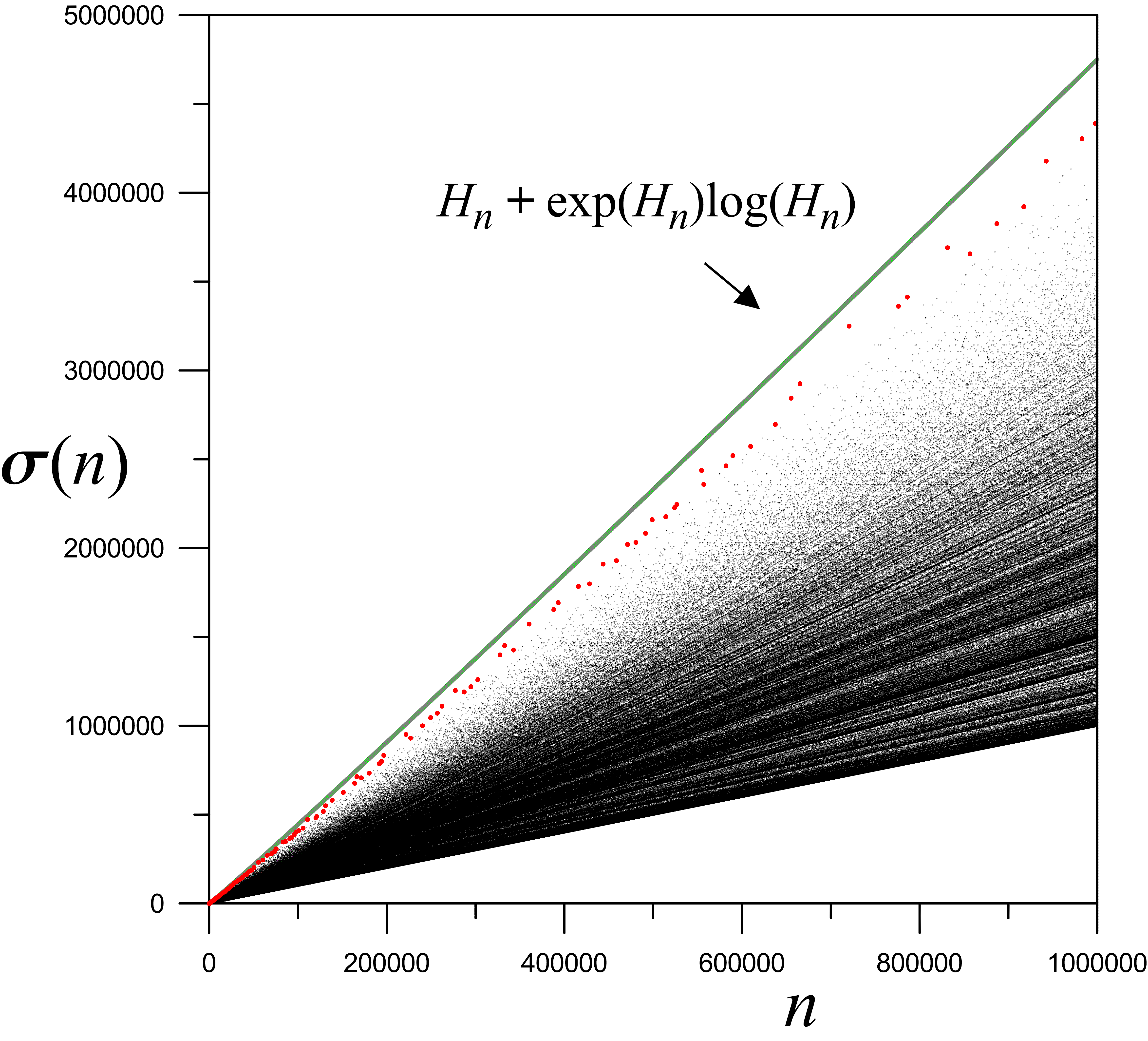
Figure 5: The plot of $\sigma(n)$ for $1<n<10^{6}$. In red are plotted values of $\sigma(n)$ which approach the threshold (green line) values closer than 10%. The lower “support” of the graph comes from $n$ being primes, as prime $p$ is divisible only by $1$ and itself, so $\sigma(p)=p+1$. Data for this plot was obtained with the free package PARI/GP [43].

Finally let us mention the elementary Lagarias criterion [44]: the Riemann Hypothesis is equivalent to the inequalities:

$$\sigma(n)\equiv\sum_{d|n}d\leq H_{n}+{\rm{e}}^{H_{n}}\log(H_{n})$$ (33)

for each $n=1,2,\ldots$, where $\sigma(n)$ is the sum of all divisors of $n$ and $H_{n}$ is the $n$-th harmonic number $H_{n}=\sum_{j=1}^{n}\frac{1}{j}$. To disprove the RH it suffices to find one $n$ violating the inequality (33). The Lagarias criterion is not well suited for computer verification (it is not an easy task to calculate $H_{n}$ for $n\sim 10^{100000}$ with sufficient accuracy) and in [45] K. Briggs has undertaken instead the verification of the Robin [46] criterion for RH:

$${\rm RH~{}~{}}\Leftrightarrow\sum_{d|n}d<e^{\gamma}n\log\log(n)~{}~{}~{}~{}{\rm for~{}~{}}n>5040.$$ (34)

For some $n$ Briggs obtained for the difference between r.h.s. and l.h.s. of the above inequality value as small as $e^{-13}\approx 2.2\times 10^{-6}$, hence again RH is in a danger to be violated. As A. Ivic has put it “The Riemann Hypothesis is a very delicate mechanism.’, quoted in [6, p. 123].

Let us notice that the belief in the validity of RH is not common: famous mathematicians J. E. Littlewood, P. Turan and A.M. Turing have believed that the RH is not true, see the paper “On some reasons for doubting the Riemann hypothesis” [47] (reprinted in [13, p.137]) written by A. Ivić, one of the present day leading expert on RH. When J. Derbyshire asked A. Odlyzko about his opinion on the validity of RH he replied “Either it’s true, or else it isn’t” [4, p. 357–358].

4 Quantum Mechanics and RH

The first physical method of proving RH was proposed by George Polya around 1914 during the conversation with Edmund Landau and now is known as the Hilbert-Polya Conjecture. Landau asked Polya: “Do you know a physical reason that the Riemann hypothesis should be true?” and his reply was: “This would be the case, I answered, if the nontrivial zeros of the $\Xi$-function were so connected with the physical problem that the Riemann hypothesis would be equivalent to the fact that all the eigenvalues of the physical problem are real”, see the whole story at the web site [48]. Let us stress that this talk took place many years before the birth of quantum mechanics and the Schroedinger equation for energy levels. However in the period 1911–1914 Hermann Weyl published a few papers on the asymptotic distribution of eigenvalues of the Laplacian in the compact domain (in particular the eigenfrequencies or natural vibrations of the drums), see e.g. [49, 50]. Thus presumably Polya was inspired by the Weyl’s papers. If the RH is true nontrivial zeros lie on critical line and it makes sense to order them according to the imaginary part and eventually put them into the 1-1 correspondence with the eigenvalues of some hermitian operator. Therefore the problem is to find a connection between energy levels $E_{n}$ of some quantum system and zeros of $\zeta(s)$.

In the autumn of 1971 [8, p.261] H. Montgomery, assuming the RH, has proved theorem about statistical properties of the spacings between zeta zeros. The formulation of this theorem is rather complicated and we will not present it here, see his paper [51]. Next Montgomery made the conjecture that correlation function of the imaginary parts of nontrivial zeros has the form (here $0<\alpha<\beta<\infty$ are fixed):

$$\sum_{\begin{subarray}{c}0<\gamma,\gamma^{\prime}\leq T\\ \frac{2\pi\alpha}{\log T}\leq\gamma-\gamma^{\prime}\leq\frac{2\pi\beta}{\log T}\end{subarray}}1\rightarrow\int_{\alpha}^{\beta}\left(1-\left(\frac{\sin\pi u}{\pi u}\right)^{2}\right)du~{}~{}~{}~{}{\rm as~{}~{}}T\rightarrow\infty.$$ (35)

In the Fig.7 we present a sketchy plot of the both sides of the equation (35). This result says that the zeros – unlike primes, where it is conjectured that there is infinity of twins primes, i.e. primes separated by 2, like $(3,5),(5,7),(11,13),\ldots,(59,61),\ldots$)— would actually repel one another because in the integrand $\sin(\pi u)/\pi u\rightarrow 1$ for $u\rightarrow 0$. Montgomery published this result in 1973 [51], but earlier in 1972 he spoke about it with F. Dyson in Princeton, see many accounts of this story in the popular books listed in the Introduction, e.g. [8, p.133–134]. Dyson recognized in (35) the same dependence as in the behavior of the differences between pairs of eigenvalues of random Hermitian matrices. The random matrices were introduced into the physics by Eugene Wigner in the fifties of twenty century to model the energy levels in the nuclei of heavy atoms. Spectra of light atoms are regular and simple in contrast to the spectra of heavy atomic nuclei, like e.g. ²³⁸U, for which hundreds of spectral lines were measured. The hamiltonians of these nuclei are not known, besides that such many body systems are too complicated for analytical treatment. Hence the idea to model heavy nuclei by the matrix with random entries chosen according to the gaussian ensemble and subjected to some symmetry condition (hermiticity etc.).

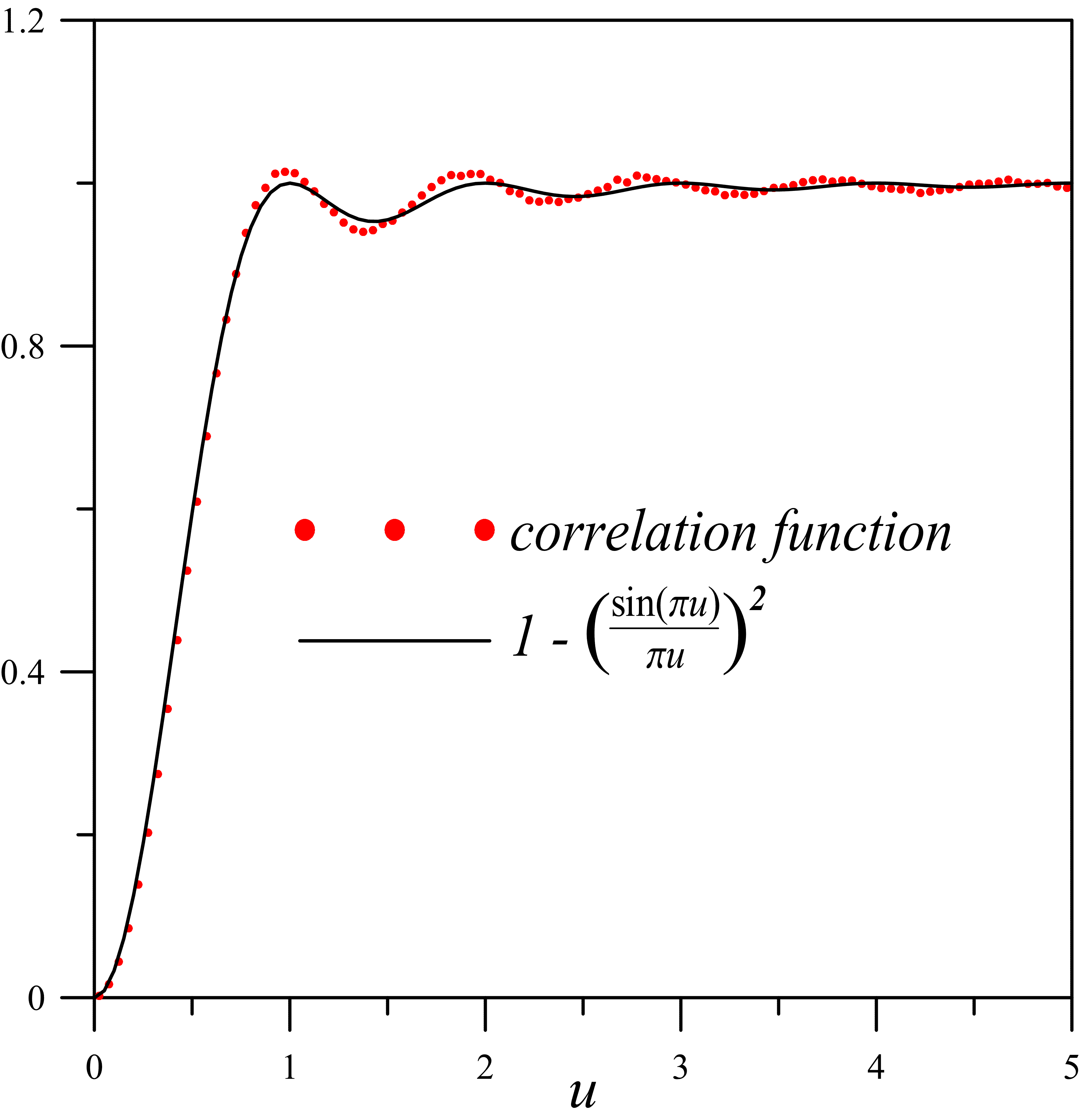
Figure 6: The plot of lhs of (35) calculated from the first $10^{7}$ zeros compared with the prediction of Montgomery. Points representing correlation function were calculated from equation on lhs of (35) for 5000000 first zeros of $\zeta(s)$ and $\Delta u=0.05$.

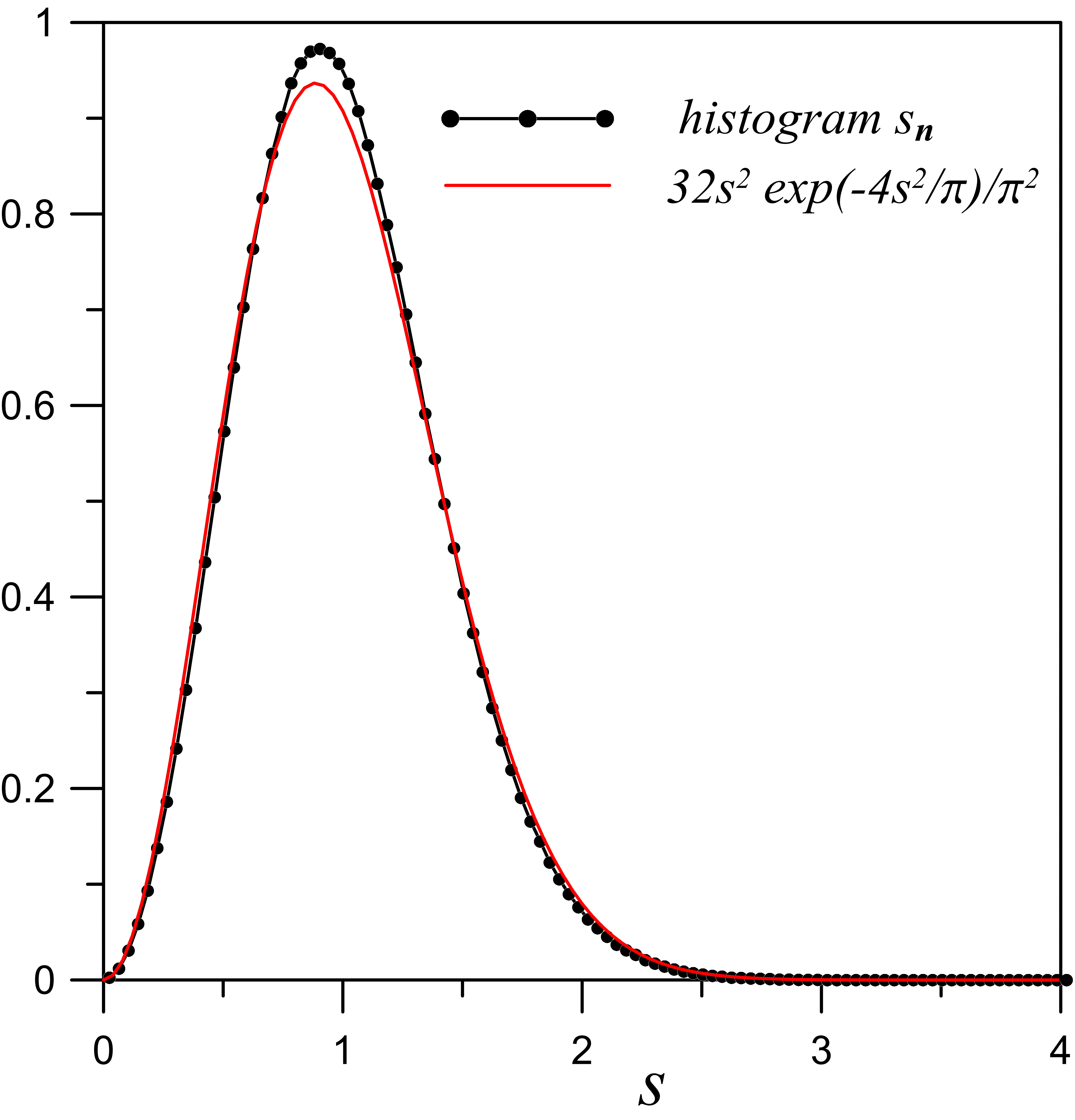
Figure 7: Histogram of normalized gaps between cinsecutive zeros of zeta obtained for 5000000 zeros. Points are spaced with $\Delta s=0.05$.

Because the hamiltonian describing interaction inside heavy nuclei is unknown Wigner proposed to use some matrix of large dimension with random entries selected with the appropriate distribution probability and subject for example to the hermiticity requirement. It means that if ${\bf M}$ is a square matrix $N\times N$ with elements $M_{ij}$, then probability $P(M_{ij}\in(a,b))$ that a given matrix element $M_{ij}$ will take value in the interval $(a,b)$ is given by the integral:

$$P(M_{ij}\in(a,b))=\int_{a}^{b}f_{ij}(x)dx,$$

where $f_{ij}$ is the density of the probability distribution and matrix elements $M_{ij}$ are mutually statistically independent, what means that the probability for the whole matrix is the product of above factors for single elements $M_{ij}$. The requirement of hermiticity (${\bf M}^{\dagger}={\bf M}$) and independence with respect to the choice of the base determine the following form, see [52, Theorem 2.6.3, p. 47]:

$$P({\bf M})=e^{-a\text{tr}\,{\bf M}^{2}+b\text{tr}\,{\bf M}+c},$$ (36)

where $a$ is a positive real number, $b$ i $c$ are real and tr denotes trace of the matrix: $\text{tr}~{}{\bf M}=\sum_{i=1}^{N}M_{ii}$. The value of $c$ is determined by normalization of the probability. For self–adjoint matrix ${\bf H}^{\dagger}={\bf H}$ we have $\text{tr}\,H^{2}=\sum_{i=1}^{N}\sum_{k=1}^{N}H_{ik}H_{ki}=\sum_{i=1}^{N}\sum_{k=1}^{N}H_{ik}H_{ik}^{\star}=\sum_{i=1}^{N}\sum_{k=1}^{N}|H_{ik}|^{2}$ and all terms in (36) have a Gaussian form. Because exponent of the sum of terms is the product of the exponents of each factors separately, the right side of the equation (36) indeed has the form of the product of the density of the normal Gaussian distributions and such a set of random, Gaussian unitary matrices is called Gaussian Unitary Ensemble, in short GUE. Eigenvalues of such matrices are not completely random: “unfolded” gaps $s$ between them are not described by the Poisson distribution $e^{-s}$, but for example for GUE by the formula

$$P(s)=\frac{32}{\pi^{2}}s^{2}e^{-4s^{2}/\pi}.$$ (37)

Unfolding means getting rid of constant trend in the spectrum $E_{1},E_{2},\ldots$, i.e. dividing $d_{n}=E_{n+1}-E_{n}$ by mean gaps between levels $\overline{d}(E)$ : $s_{n}=(E_{n+1}-E_{n}))/\overline{d}(E)$. For zeros of $\zeta(s)$ from equation (23) the differences $\gamma_{n+1}-\gamma_{n}$ are changed into $s_{n}=(\gamma_{n+1}-\gamma_{n})\log(\gamma_{n})/2\pi$. In the Fig.7 we show the comparison of (37) with real gaps for zeros of $\zeta(s)$.

Level-spacing distributions of quantum systems can be grouped into a few universality classes connected with the symmetry properties of the Hamiltonians: Poisson distribution for systems with underlying regular classical dynamics, Gaussian orthogonal ensemble (GOE, also called the Wigner -Dyson distribution) — Hamiltonians invariant under time reversal, Gaussian unitary ensemble (GUE) — not invariant under time reversal and Gaussian symplectic ensemble (GSE) for half-spin systems with time reversal symmetry. There are many reviews on these topics, we cite here [52], [53], [54], we strongly recommend the review [55]. Dyson and Mehta identified these three types of random matrices with different intensities of repulsion spacings between consecutive energy levels : GOE with weakest repulsion between neighboring levels, GUE with medium repulsion and GSE with strongest repulsion. For quantitative description see [56, Appendix A].

For several years discovered during a brief conversation of Montgomery with Dyson relationship of nontrivial zeros $\zeta(s)$ with the eigenvalues of matrix from the GUE did not arouse much interest. In the eighties of previous century Andrew Odlyzko performed over many years computation of zeta zeros in different intervals and calculated their pair-correlation function numerically. In the first paper [57] he tested Montgomery pair correlation conjecture for first 100,000 zeros and for zeros number $10^{12}$ to $10^{12}+100,000$. Next he looked at $10^{20}$-th zero of the Riemann zeta function and 70 million of its neighbors, the $10^{20}$-th zero of the Riemann zeta function and 175 million of its neighbors, last searched interval was around zero $10^{22}$ and involved $10^{9}$ zeros, see [29]. The reason Odlyzko investigated zeros further and further is the very slow convergence of various characteristics of $\zeta(s)$ to its asymptotic behavior. The results confirmed the GUE distribution: the gaps between imaginary parts of consecutive nontrivial zeros of $\zeta(s)$ display the same behavior as the differences between pairs of eigenvalues of random Hermitian matrices, see [57, Fig.1 and Fig.2]. In [58, p.146] Peter Sarnak wrote: “At the phenomenological level this is perhaps the most striking discovery about the zeta function since Riemann.” In this way vague hypothesis of Hilbert - Polya has gained credibility and now it is known that a physical system corresponding to $\zeta(s)$ has to break the symmetry with respect to time reversal. At the conference “Quantum chaos and statistical nuclear physics” held in Cuernavaca, Mexico, in January 1986 Michael Berry delivered the lecture Riemann s zeta function: a model for quantum chaos? [59] which became the manifesto of the approach to prove the RH which can be summarized symbolically as $\zeta(\frac{1}{2}+i\hat{H}_{R})=0$ with $\hat{H}_{R}$ a hermitian operator having as eigenvalues imaginary parts of nontrivial zeros $\gamma_{k}$: $\hat{H}_{R}|\Psi_{k}\rangle=\gamma_{k}|\Psi_{k}\rangle$. The hypothetical quantum system (fictitious element) described by such a hamiltonian was dubbed by Oriol Bohigas “Riemannium”, see [60, 61]. Additionally to the lack of time reversal invariance of $\hat{H}_{R}$ Berry in [59] pointed out that $\hat{H}_{R}$ should have a classical limit with classical orbits which are all chaotic (unstable and bounded trajectories). In fact the departure of correlation function for zeta zeros from (35) for large spacings (argument larger than 1 in [57, Fig.1 and Fig.2]) was a manifestation of quantum chaos, as Berry recognized. Later on M. Berry and J. Keating have argued [62] that $\hat{H}_{R}=xp$. The main argument for connection of $\hat{H}_{R}=xp$ with the RH was the fact, that the number of states of this hamiltonian with energy less than $E$ is given by the formula:

$$N(E)=\frac{E}{2\pi}\left(\log\left(\frac{E}{2\pi}\right)-1\right)+\frac{7}{8}+\ldots$$

what exactly coincides with (23). In the derivation of above result Berry and Keating “cheated” using very special Planck cell regularization to avoid infinite phase–space volume. As a caution we mention here an example of a very special shape billiard for which the formula for a number of energy levels below $E$ has a leading term exactly the same as for zeta function (23) but the next terms disagree, see [63, eqs. (34–35)]. We remind here that two drums can have different shapes but identical eigenvalues of vibrations, thus the same spectral staircase function. In 2011 S. Endres and F. Steiner [64] showed that spectrum of $\hat{H}_{R}=xp$ on the positive $x$ axis is purely continuous and thus $\hat{H}_{R}=xp$ cannot yield the hypothetical Hilbert -Polya operator possessing as eigenvalues the nontrivial zeros of the $\zeta(s)$ function. The choice $\hat{H}_{R}=xp$ for the operator of Riemannium possesses some additional drawbacks (e.g. it is integrable, and therefore not chaotic) and some modification of it were proposed, see series of papers by G. Sierra e.g. [65, 66].

In August 1998, during a conference in Seattle devoted to 100–th anniversary of the PNT, Peter Sarnak offered a bottle of good wine for physicists who will be able to recover some information from the Montgomery - Odlyzko conjecture that is not formerly known to mathematicians. Just two years later he had to go to the store to buy promised wine. At the conference in Vienna in September 1998, Jon Keating delivered a lecture during which he announced solution (but no proof) of the so called problem of moments of zeta. These results were published later in a joint work with his PhD student Nina Snaith [67]. For nearly a hundred years mathematicians have tried to calculate moments of the zeta function on the critical line

$$\frac{1}{T}\int_{0}^{T}|\zeta(\tfrac{1}{2}+\imath t)|^{2k}dt,~{}~{}~{}~{}~{}~{}\text{for }T\rightarrow\infty$$ (38)

G.H. Hardy and J.E. Littlewood [68, Theorem. 2.41] calculated the second moment:

$$\frac{1}{T}\int_{0}^{T}|\zeta(\tfrac{1}{2}+\imath t)|^{2}dt\sim\log(T),~{}~{}~{}~{}~{}\text{for }T\rightarrow\infty.$$ (39)

The fourth moment calculated A.E. Ingham in 1926 [69, Th. B]

$$\frac{1}{T}\int_{0}^{T}|\zeta(\tfrac{1}{2}+\imath t)|^{4}dt\sim\tfrac{1}{2\pi}\log^{4}(T),~{}~{}~{}~{}~{}\text{for }T\rightarrow\infty.$$ (40)

Higher moments, despite many efforts, were not known, but it was supposed for $k=3$ [70] that:

$$\int_{1}^{T}|\zeta(\tfrac{1}{2}+it)|^{6}~{}dt\sim\frac{42}{9!}\prod_{p}\left\{\left(1-\frac{1}{p}\right)^{4}\left(1+\frac{4}{p}+\frac{1}{p^{2}}\right)\right\}T\log^{9}T\text{~{}~{} for large }T,$$ (41)

and even more complex expression for $k=4$ [71].

$$\int_{0}^{T}|\zeta(1/2+it)|^{8}~{}dt\sim\frac{24024}{16!}\prod_{p}\left(\left(1-\frac{1}{p}\right)^{9}\left(1+\frac{9}{p}+\frac{9}{p^{2}}+\frac{1}{p^{3}}\right)\right)T\log^{16}T.$$ (42)

Keating and Snaith proved the general theorem for moments of random matrices, which eigenvalues have GUE distribution and if the behavior of $\zeta(s)$ is modeled by the determinant of such a matrix, then their result applied to the zeta gives

$$\frac{1}{T}\int_{0}^{T}\left|\zeta(\tfrac{1}{2}+\imath t)\right|^{2k}\;dt\sim f_{k}a(k)(\log T)^{k^{2}},$$ (43)

where

$$a(k)=\prod_{p}\left(1-\frac{1}{p}\right)^{k^{2}}\sum_{m=0}^{\infty}\left(\frac{\Gamma(m+k)}{m!\,\Gamma(k)}\right)^{2}p^{-m},$$ (44)

and numbers $f_{k}$ are given by

$$f_{k}=\frac{G^{2}(k+1)}{G(2k+1)}.$$

In the above formula $G(\cdot)$ is the Barnes function satisfying the recurrence $G(z+1)=\Gamma(z)G(z)$ with starting value $G(1)=1$, thus for natural arguments this function is a “factorial over factorials”: $G(n)=1!\cdot 2!\cdot 3!\ldots(n-2)!$. Of course, the result of Keating and Snaith gives formulas (39)–(42), respectively for $k=1,2,3,4$.

In [72] P. Crehan has shown that for any sequence of energy levels obeying a certain growth law ($|E_{n}|<e^{an+b}$, for some $a\in\mathbb{R}^{+}$, $b\in\mathbb{R}$), there are infinitely many classically integrable Hamiltonians for which the corresponding quantum spectrum coincides with this sequence. Because from PNT it follows, that the $n-$th prime $p_{n}$ grows like $p_{n}\sim n\log(n)$ the results of Crehan’s paper can be applied and there exist classically integrable hamiltonians whose spectrum coincides with prime numbers, see also [73]. From (23) it follows that the imaginary part of the $n$–th zero of $\zeta(s)$ grows like $\gamma_{n}\sim 2\pi n/\log(n)$, thus the theorem of Crehan can be applied and it follows that there exists an infinite family of classically integrable nonlinear oscillators whose quantum spectrum is given by the imaginary part of the sequence of zeros on the critical line of the Riemann zeta function.

In the end of XX centaury there were a lot of rumors that Allain Connes has proved the RH using developed by him noncommutative geometry. Connes [74] constructed a quantum system that has energy levels corresponding to all the Riemann zeros that lie on the critical line. To prove RH it has to be shown that there are no zeros outside critical line, i.e. unaccounted for by his energy levels. The operator he constructed acts on a very sophisticated geometrical space called the noncommutative space of adele classes. His approach is very complicated and in fact zeros of the zeta are missing lines (absorption lines) in the continuous spectra. During the passed time excitement around Connes s work has faded and much of the hope that his ideas might lead to the proof of RH has evaporated. The common opinion now is that he has shifted the problem of proving the RH to equally difficult problem of the validity of a certain trace formula.

We mention also the paper written by S. Okubo[75] entitled “Lorentz-Invariant Hamiltonian and Riemann Hypothesis”. It is not exactly the realization of the idea of Polya and Hilbert: the appearing in this paper two dimensional differential operator (hamiltonian $H$) does not possess as eigenvalues imaginary parts of the nontrivial zeros of the $\zeta(s)$. Instead the special condition for zeros of zeta function is used as the boundary condition for solutions of the eigenvalue equation $H|\phi\rangle=\lambda|\phi\rangle$. Unfortunately, the obtained eigenfunctions are not normalizable.

Let us remark that for trivial zeros $-2n$ of $\zeta(s)$ with a constant gap 2 between them it is possible to construct hamiltonian reproducing these zeros as eigenvalues. Namely, the eigenvalue problem for the harmonic oscillator in the units $m=\hbar=\omega=1$ has the form:

$$\frac{1}{2}\left(-\frac{d^{\,2}}{dx^{2}}+x^{2}\right)\psi_{n}(x)=(n+\tfrac{1}{2})\psi_{n}(x)$$ (45)

where

$$\psi_{n}(x)=e^{-\tfrac{x^{2}}{2}}\cdot H_{n}(x),\qquad n=0,1,2,\ldots$$

and $H_{n}(x)$ are Hermite polynomials:

$$H_{n}(x)=(-1)^{n}e^{x^{2}}\frac{d^{n}}{dx^{n}}\left(e^{-x^{2}}\right).$$

Multiplying (45) by $-2$ and rearranging terms we obtain

$$\left(\frac{d^{\,2}}{dx^{2}}-x^{2}+1\right)\psi_{n}(x)=-2n\psi_{n}(x).$$

Hence the hamiltoniam for trivial zeros of $\zeta(s)$ is

$$\hat{H}_{triv}=\frac{d^{\,2}}{dx^{2}}-x^{2}+1.$$

Since the advent of quantum computers and the discovery by Peter Shor of the quantum algorithm for integer factorization [76] there is an interest in applying these algorithms to diverse of problems. Is it possible to devise the quantum computer verifying the RH? We mean here something more clever than, say, simply mixing the Shor’s algorithm with Lagarias criterion. Recently there appeared the paper [77], in which authors (assuming the RH) have built an unitary operator with eigenvalues equal to combination of nontrivial zeros $\overline{\rho_{j}}/\rho_{j}$ lying on the unit circle. Next the quantum circuit representing this unitary matrix is constructed. Recently in [78, p. 4] the quantum computer verifying RH was proposed, but it seems to us to be artificial and not sufficiently sophisticated: it is based on the (26) and it counts in a quantum way actual number of prime numbers below $x$ and looks for departures beyond the bound in (26).

We do not have space here to discuss the use of $\zeta(s)$ in the theory of Casimir effect — devoted to this subject is the extensive review by K. Kirsten in [79], or in string theory [80, 81].

5 Statistical Mechanics and RH

The partition function $Z(\beta)$ is the basic quantity used in statistical physics, here $\beta=1/k_{B}T$: $k_{B}=1.3806488\ldots\times 10^{-23}$[J/K] is the Boltzmann constant and $T$ is the absolute temperature. All thermodynamical functions can be expressed as derivatives of $Z(\beta)$. The phase transitions appear at such temperatures that $Z(\beta)=0$. For the system, which may be in micro–states with energy $E_{n}$ and can exchange heat with environment and with fixed number of particles, volume and temperature, the partition function is given by the formula:

$$Z(\beta)=\sum_{n}e^{-\beta E_{n}}.$$ (46)

It turns out that for certain systems $Z(\beta)$ satisfies the relation similar to functional equation for $\zeta(s)$ and positions of zeros of the partition function analytically continued to the whole complex plane are highly restricted, for example to the circle. These two facts have become the starting point for attempts to prove HR.

It is very easy to construct the system with the $\zeta(s)$ as a partition function. The problem of construction of a simple one–dimensional Hamiltonian whose spectrum coincides with the set of primes was considered in [82], [83], [84], see also review [73]. Some modification should lead to the Hamiltonian $H$ having eigenstates $|p\rangle$ labeled by the prime numbers $p$ with eigenvalues $E_{p}=\mathcal{E}\log(p)$, where $\mathcal{E}$ is some constant with dimension of energy. The $n$ particle state can be decomposed into the states $|p\rangle$ using the factorization theorem (5). The energy of the state $|n\rangle$ is equal to $E(n)=\mathcal{E}\sum_{i=1}^{k}\alpha_{i}\log(p_{i})=\mathcal{E}\log(n)$. Then the partition function $Z$ is given by the Riemann zeta function:

$$Z(T)=\sum_{n=1}^{\infty}\exp\left(\frac{-E_{n}}{k_{B}T}\right)=\sum_{n=1}^{\infty}\exp\left(\frac{-\mathcal{E}\log n}{k_{B}T}\right)=\sum_{n=1}^{\infty}\frac{1}{n^{s}}=\zeta(s),~{}~{}~{}~{}s\equiv\mathcal{E}/k_{B}T$$

Such a gas was considered e.g. in [18] and [85] and found applications in the string theory.

The functional equation (15) can be written in non–symmetrical form:

$$2\Gamma(s)\cos\big{(}\frac{\pi}{2}s\big{)}\zeta(s)=(2\pi)^{s}\zeta(1-s).$$

In this form it is analogous to the Kramers–Wannier [86] duality relation for the partition function $Z(J)$ of the two dimensional Ising model with parameter $J$ expressed in units of $k_{B}T$ (i.e. equal to interaction constant multiplied by $\beta=1/k_{B}T$)

$$Z(J)=2^{N}(\cosh(J))^{2N}(\tanh(J))^{N}Z(\widetilde{J}),$$ (47)

where $N$ denotes the number of spins and $\widetilde{J}$ is related to $J$ via $e^{-2\widetilde{J}}=\tanh(J)$, see e.g. [87]. On the other hand there are so called “Circle theorems” on the zeros of partition functions of some particular systems. To pursue this analogy one has to express the partition function by the $\zeta(s)$ function. Then one can hope to prove RH by invoking the Lee–Yang circle theorem on the zeros of the partition function. The Lee–Yang theorem concerns the phase transitions of some spin systems in external magnetic field and some other models (for a review see [88]). Let $Z(\beta,z)$ denote the grand – canonical partition function, where $z=e^{\beta H}$ is the fugacity connected with the magnetic field $H$. Phase transitions are connected with the singularities of the derivatives of $Z(\beta,z)$, and they appear when $Z(\beta,z)$ is zero. The finite sum defining $Z(\beta,z)$ can not be a zero for real $\beta$ or $z$ and the Lee–Yang theorem [89, 90] asserts that in the thermodynamical limit, when the sum for partition function involves infinite number of terms, all zeros of $Z(\beta,z)$ for a class of spin models are imaginary and lie in the complex plane of the magnetic field $z$ on the unit circle: $|z|=1$. The study of zeros of the canonical ensemble in the complex plane of temperature $\beta$ was initiated by M.Fisher [91]. He found in the thermodynamic limit for a special Ising model not immersed in the magnetic field, that the zeros of the canonical partition function also lie on an unit circles, this time in the plane of the complex variable $v=\sinh(2J\beta)$, where $J>0$ is the ferromagnetic coupling constant. The critical line $s=\frac{1}{2}+it$ can be mapped into the unit circle via the transformation $s\rightarrow u=s/(1-s)=(\frac{1}{2}+it)/(\frac{1}{2}-it)$ because then $|u|=1$. Thus by devising appropriate spin system with $Z(\beta,z)$ expressed by the $\zeta(s)$ the Lee–Yang theorem can be used to locate the possible zeros of the latter function and lead to the proof of RH.

In the series of papers A. Knauf [92, 93, 94] has undertaken the above outlined plan to attack the RH. In these papers he introduced the spin system with the partition function in the thermodynamical limit expressed by zeta function: $Z(s)=\zeta(s-1)/\zeta(s)$ with $s$ interpreted as the inverse of temperature. However the form of interaction between spins in his model does not belong to one of the cases for which the circle theorem was proved. This idea was further developed in paper [95]. The authors of the paper [96] have shown that RH is equivalent to an inequality satisfied by the Kubo -Martin -Schwinger states of the Bost and Connes quantum statistical dynamical system in special range of temperatures. There are many other appearances of the $\zeta(s)$ in the statistics of bosons and fermions, theory of the Bose–Einstein condensate, some special “number theoretical” gases etc, for introduction see [14, chap. III E].

6 Random walks, billiards, experiments etc.

The Möbius function defined in (10) takes only three values: -1, 0 and 1. The values $\mu(n)=1$ and $\mu(n)=-1$ are equiprobable with probabilities $3/\pi^{2}\approx 0.3039$, thus the probability of value $\mu(n)=0$ is $1-6/\pi^{2}\approx 0.3921$. Using values 1 and -1 of the Möbius function instead of heads or tails of a coin should hence generate a symmetric one-dimensional random walk. The total displacement during $n$ steps of such a random walk will be given by the summatory function of the Möbius function: $M(x)=\sum_{n<x}\mu(n)$, which is called the Mertens function. It is well known that the “root mean square” distance from the starting point of the symmetrical random walk during $N$ steps grows like $\sqrt{N}$. The resemblance of $M(n)$ to the symmetrical random walk led F. Mertens in the end of XIX century to make the conjecture that $M(n)$ grows not faster than the mean displacement of the symmetrical random walk, i.e. $|M(n)|<\sqrt{n}$. It is an easy calculation to show that Mertens conjecture implies the RH (vide (11)):

$$\frac{1}{\zeta(s)}=\sum_{n=1}^{\infty}\frac{\mu(n)}{n^{s}}=\sum_{n=1}^{\infty}\frac{M(n)-M(n-1)}{n^{s}}=\sum_{n=1}^{\infty}M(n)\left(\frac{1}{n^{s}}-\frac{1}{(n+1)^{s}}\right)=$$

$$=\sum_{n=1}^{\infty}M(n)\int_{n}^{n+1}\frac{sdx}{x^{s+1}}=s\sum_{n=1}^{\infty}\int_{n}^{n+1}\frac{M(x)dx}{x^{s+1}}=s\int_{1}^{\infty}\frac{M(x)dx}{x^{s+1}}.$$

If $M(x)<\sqrt{x}$ then the last integral above gives $\left|\frac{1}{\zeta(s)}\right|<\frac{|s|}{\sigma-\frac{1}{2}}$, thus to the right of the line $\Re[s]=\frac{1}{2}$ the inverse of zeta function is bounded hence there can not be zeros of $\zeta(s)$ in this region and the truth of RH follows. For many years mathematicians hoped to prove the RH by showing the validity of $|M(n)|<\sqrt{n}$. However in 1985 A. Odlyzko and H. te Riele [97] disproved the Mertens conjecture; in the proof they have used values of first 2000 zeros of $\zeta(s)$ calculated with accuracy 100–105 digits; these calculations took 40 hours on CDC CYBER 750 and 10 hours on Cray-1 supercomputers. Using Mathematica these computations can be done on the modern laptop in a couple of minutes. Littlewood proved that the RH is equivalent to slightly modified Mertens conjecture

$$M(n)={\mathcal{O}}(n^{1/2+\epsilon})\Leftrightarrow{\rm RH~{}is~{}true}.$$

The fact that $M(n)$ behaves like a one dimensional random walk was also pointed out in [98] and used to show that RH is “true with probability 1”.

In the paper [99] M. Shlesinger has investigated a very special one-dimensional random walk which can be linked with the RH. The probability of jumping to other sites with steps having a displacement of $\pm l$ sites involves directly the Möbius function:

$$p(\pm{\rm\textit{l}})=\frac{1}{2}C\left(\frac{1}{\rm{\textit{l}}^{~{}1+\beta}}\pm\frac{\mu(\rm{\textit{l}})}{\rm{\textit{l}}^{~{}1+\beta-\epsilon}}\right),~{}~{}~{}~{}\beta>0,$$

where $C=\frac{1}{\zeta(1+\beta)+\frac{1}{\zeta(1+\beta)}}$ is a normalization factor, $\beta$ (to be not confused with $\beta=1/k_{B}T$) is the fractal dimension of the set of points visited by random walker. He coined the name Riemann–Möbius for this random walk. Some general properties of the ”structure function” $\lambda(k)$ being the Fourier of the probabilities $p(l)$: $\lambda(k)=\sum_{l}e^{ikl}p(l)$, enabled Shlesinger to locate the complex zeros inside the critical strip, however the result of J. Hadamard and Ch. J. de la Vall e–Poussin that $\zeta(1+it)\neq 0$ can not be recovered by this method. What is interesting the existence of off critical line zeros is not in contradiction with behavior of $\lambda(k)$ following from the universal laws of probability.

In [100] the stochastic interpretation of the Riemann zeta function was given. There are much more connections between $\zeta(s)$ and random walks as well as Brownian motions known to mathematicians. The extensive review of obtained results expressing expectation values of different random variables by $\zeta(s)$ or $\xi(s)$ can be found in [101].

In the paper [102] L.A. Bunimovich and C.P. Dettmann considered the point particle bouncing inside the circular billiard. There is a possibility that the small ball will escape through a small hole on the reflecting perimeter. Let $P_{1}(t)$ denote the probability of not escaping from a circular billiard with one hole till time $t$. Bunimovich and Dettmann obtained exact formula for $P_{1}(t)$ and surprisingly this probability was expressed by $\zeta(s)$. So here again the function of purely number theoretical origin meets the physical reality. Then they proved that RH is equivalent to

$$\lim_{\epsilon\to 0}\lim_{t\to\infty}\epsilon^{\delta}(tP_{1}(t)-2/\epsilon)=0$$ (48)

be true for every $\delta>-1/2$. Here this value $1/2$ is directly connected with the location of critical line in the formulation of RH. A little bit more complicated condition was obtained for biliard with two holes. In principle such conditions allow experimental verification of RH using microwave cavities simulating billiards or optical billiards constructed with microlasers. Experiments can refute RH if the behavior of $tP_{1}(t)-2/\epsilon$ in the limit $\epsilon\to 0$ will be slower than power like dependence $\epsilon^{1/2}$ in the limit of vanishing $\epsilon$. To our knowledge up today no such experiments were performed. In the paper [103] generalization to the spherical billiard was considered. Again the survival probability in such a 3D biliard is related to the Riemann hypothesis.

Already in 1947 van der Pol has built the electro–mechanical device verifying the RH [104]. He has built machine plotting the $\zeta(1/2+it)$ from the following integral representation:

$$\frac{\zeta(\frac{1}{2}+it)}{\frac{1}{2}+it}=\int_{-\infty}^{\infty}\left(e^{-x/2}\lfloor e^{x}\rfloor-e^{x/2}\right)e^{-ixt}dx.$$ (49)

Here $\lfloor x\rfloor$ denotes integer part of $x$. It has the form of Fourier transform of the function $y(x)=e^{-x/2}\lfloor e^{x}\rfloor-e^{x/2}$. The plot of integrand is shown in Fig. 8. The shape of this function was cut precisely with scissors on the edge of a paper disc. The beam of light was passing between teeth on the perimeter of the disc and detected by the photocell. The resulting from photoelectric effect current was superimposed with current of varying frequency to perform analogue Fourier transform. After some additional operations van der Pol has obtained the plot of modulus $|\zeta(\frac{1}{2}+it)/\frac{1}{2}+it|$ on which the first 29 nontrivial zeta zeros were located with accuracy better than %1. The authors of [14] have summarized this experiment in the words: “This construction, despite its limited achievement, deserves to be treated as a gem in the history of the natural sciences.”.

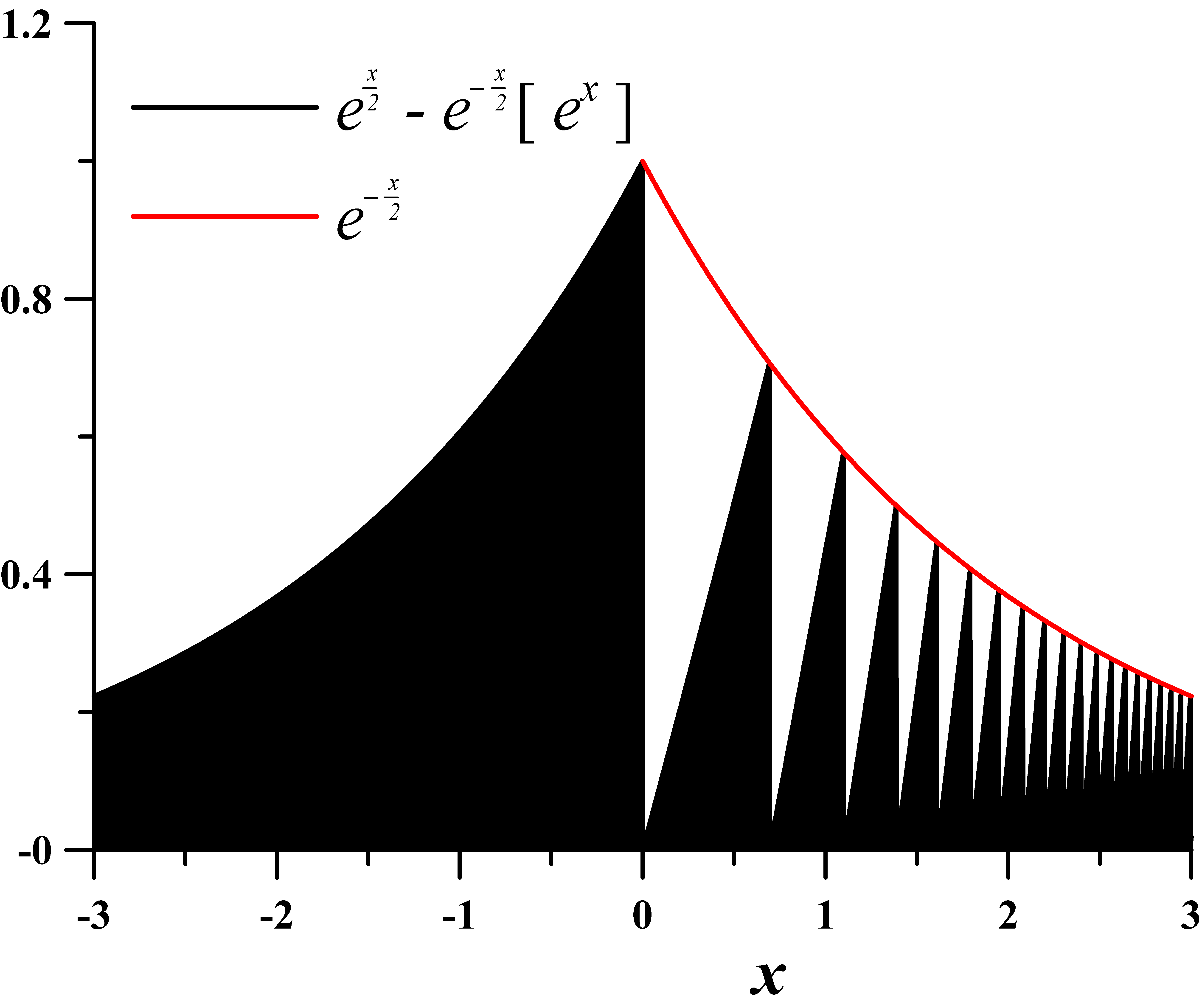
Figure 8: Plot of the function appearing in the integral representation (49) of the zeta function.

It is well known that two–dimensional electrostatic fields can be found using the functions of complex variables. There arises a question to which electrostatic problem the zeta function can be linked? In the recent paper [105] A. LeClair has developed this analogy and he constructed a two–dimensional vector field $\overrightarrow{E}$ from the real and imaginary parts of the zeta function. It allowed him to derive the formula for the $n$-th zero on the critical line of $\zeta(s)$ for large $n$ expressed as the solution of a simple transcendental equation.

In the written [106] version of his AMS Einstein Lecture “Birds and frogs” (which was to have been given in October 2008 but which unfortunately had to be canceled) Freeman Dyson points to the possibility of proving the RH using the similarity in behavior between one–dimensional quasi-crystals and the zeros of the $\zeta(s)$ function. If RH is true then locations of its nontrivial zeros would define a one–dimensional quasi–crystal but the classification of them is still missing.

7 Zeta is a fractal

In 1975 S.M. Voronin [107] proved remarkable theorem on the universality of the Riemann $\zeta(s)$ function.

Voronin’s theorem: Let $0<r<1/4$ and $f(s)$ be a complex function continuous for $|s|\leq r$ and analytical in the interior of the disk. If $f(s)\neq 0$, then for every $\epsilon>0$ there exists real number $T=T(\epsilon,f)$ such that:

$$\max_{|s|\leq r}\;\left|f(s)-\zeta\left(s+\left(\frac{3}{4}+i\;T\right)\right)\right|<\epsilon.$$ (50)

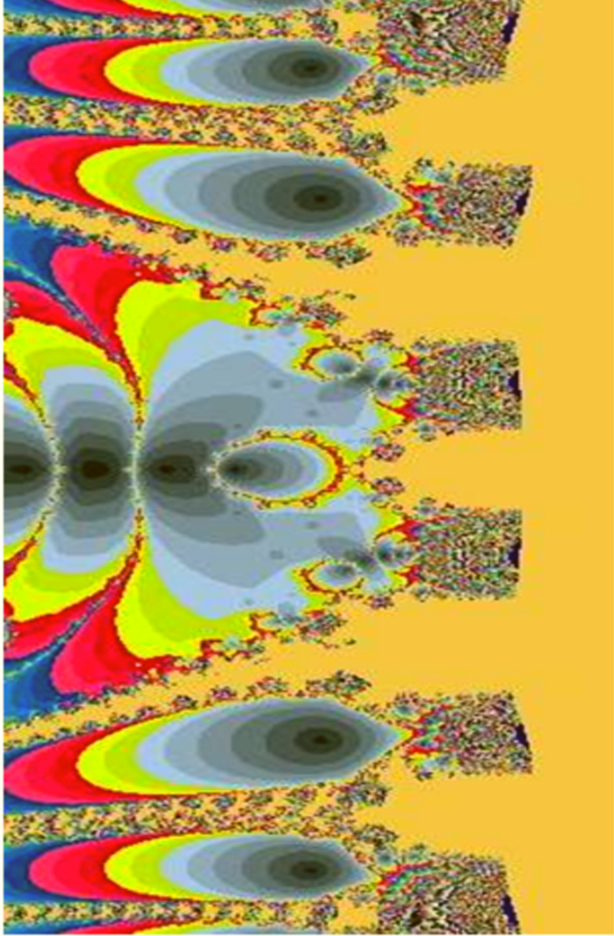
Figure 9: The plot of initial values for (51) $-9<\Re(z_{0})<9,-25<\Im(z_{0})<25$ showing in colors the number $n$ of iterations of (51) after which $|\zeta(z_{n})|<0.000001$. In black are shown regions around zeros of zeta. Clearly are visible zeros: -2, -4, -6, -8 and nontrivial $\frac{1}{2}\pm i14.134\ldots,\frac{1}{2}\pm i21.022\ldots$.

Put simply in words it means that the zeta function approximates locally any smooth function in a uniform way! By applying this theorem to itself, i.e. taking as $f(s)=\zeta(s)$, we obtain that $\zeta(s)$ is selfsimilar, see S.C. Woon [108] who has shown that the Riemann $\zeta(s)$ is a fractal. In the paper [109] the Voronin’s theorem was applied to the physical problem: to propose a new formulation of the Feynman s path integral.

Another aspect of fractality of zeta was found in [110, 84], where the one–dimensional quantum potential was numerically constructed from known zeta zeros which in turn are reproduced as eigenvalues of this potential. The fractal dimension of the graph of this potential was determined to be around 1.5. In [84] even the multifractal nature of this potential was revealed.

In the late seventies of XX centaury John Hubbard has analysed the Newton’s method for finding approximations to the roots of equation $f(x)=0$ to the case of polynomial $z^{3}-1$ on the complex plane. In this method the root $x^{\star}$ of $f(x^{\star})=0$ is obtained as a limit $x^{\star}=\lim_{n\rightarrow\infty}x_{n}$ of the sequence:

$$x_{n+1}=x_{n}-\frac{f(x_{n})}{f^{\prime}(x_{n})}.$$

If the function $f(x)$ has a few roots the limit depends on the choice of the initial $x_{0}$. Hubbard was interested in the question which starting points $z_{0}\in\mathbb{C}$ tend to one of three roots $1,(-1\pm\sqrt{3}i)/2$ of $z^{3}=1$. He obtained one of the first fractal images full of interwoven corals. Tomoki Kawahira has applied Newton’s method to the Riemann’s zeta function:

$$z_{n+1}=z_{n}-\frac{\zeta(z_{n})}{\zeta^{\prime}(z_{n})}.$$ (51)

Because $\zeta(s)$ has infinitely many roots, instead of looking for basin domains of different zeta zeros, he looked for the number of iterations of (51) for a given starting point $z_{0}$ needed to fall into the close vicinity of one of the zeros. Let us mention that such a modification was also applied to the original problem $z^{3}=1$. He obtained beautiful pictures representing the zeros of $\zeta(s)$. We present in Fig. 9 the plot obtained by M. Dukiewicz [111].

8 Concluding Remarks

We have given many examples of physical problems connected to the RH. In XIX centaury all these problems were not known, but it seems that Riemann believed that the questions of mathematics could be answered with the help of physics and in fact he performed some physical experiments by himself to check some of his theorems, see [112]. We add here, that there is a wide spread rumor among the people who are trying to solve the RH that Fields Medal Laureate Enrico Bombieri believes that RH will be proved by a physicist, see [8, p. 4].

Some mathematicians enunciate the opinion that RH is not true because long open conjectures in analysis tend to be false. In other words nobody has proved RH because simply it is not true. There are examples from number theory when some conjectures confirmed by huge “experimental” data finally turned out to be false and possible counterexamples are so large that never will be accessible to computers. One such common belief was the inequality ${\rm{Li}}(x)>\pi(x)$ remarked already by Gauss and confirmed by all available data, now it is about $x=10^{18}$. However, in 1914 J.E. Littlewood has shown [113] that the difference between the number of primes smaller than $x$ and the logarithmic integral up to $x$ changes the sign infinitely many times, what was another rather complicated proof of the infinitude of primes. The smallest value $x_{S}$ such that for the first time $\pi(x_{S})\geq{\rm{Li}}(x_{S})$ holds is called Skewes number because in 1933 S. Skewes [114], assuming the truth of the Riemann hypothesis, argued that it is certain that $\pi(x)-{\rm{Li}}(x)$ changes sign for some $x_{S}<10^{10^{10^{34}}}$. In 1955 Skewes [115] has found, without assuming the Riemann hypotheses, that $\pi(x)-{\rm{Li}}(x)$ changes sign at some $x_{S}<\exp\exp\exp\exp(7.705)<10^{10^{10^{10^{3}}}}$. This enormous bound for $x_{S}$ was several times lowered and the lowest present day known estimation of the Skewes number is around $10^{316}$, see [116] and [117]. The second example is provided by the Mertens conjecture discussed in Sect.6. The inequality $|M(x)|<x^{\frac{1}{2}}$ is confirmed by all available data but finally it is false. Like in the case of the inequality $\pi(x)>{\rm{Li}}(x)$ we can expect first $x$ for which $|M(x)|>x^{\frac{1}{2}}$ at horribly heights. Namely J. Pintz [118] has shown that the first counterexample appears below $\exp(3.21\times 10^{64})$. This upper bound was later lowered to $\exp(1.59\times 10^{40})$ [119]. Such examples show that confirmation of some facts up to say $10^{18}$ is misleading and somewhere at $t=10^{10^{\iddots}}$ the nontrivial zero of $\zeta(s)$ with real part different from $\frac{1}{2}$ can be lurking.

Acknowledgement: I thank Magdalena Dukiewicz–Jurka for allowing me to use the Fig. 9 from her master thesis (performed under my guidance in 2006). I thank Magdalena Załuska–Kotur and Jerzy Cisło for comments and remarks.

References

- [1] D. Zagier, “The first 50 million prime numbers,” Mathematical Intelligencer, vol. 0, pp. 7–19, 1977.
- [2] D. Hilbert, “Mathematical problems. Lecture Delivered Before The International Congress Of Mathematicians At Paris In 1900,” Bull. Amer. Math. Soc., vol. 8, pp. 437–479, 1992.
- [3] A. H. Helfgott, “The ternary Goldbach problem,” arXiv: math.NT/1501.05438, Jan. 2015.
- [4] J. Derbyshire, Prime Obsession. Bernhard Riemann and the greatest unsolved problem in mathematics. Washington: Joseph Henry Press, 2003.
- [5] K. Sabbagh, The Riemann hypothesis : the greatest unsolved problem in mathematics. New York: Farrar, Straus, and Giroux, 2002.
- [6] K. Sabbagh, Dr. Riemann’s Zeros: The Search for the $1 million Solution to the Greatest Problem in Mathematics. Atlantic Books, November 2002.
- [7] D. Rockmore, Stalking the Riemann hypothesis : the quest to find the hidden law of prime numbers. New York: Pantheon Books, 2005.
- [8] M. Sautoy, The music of the primes: searching to solve the greatest mystery in mathematics. New York: HarperCollins, 2003.
- [9] E. C. Titchmarsh, The Theory of the Riemann Zeta-function. New York: The Clarendon Press Oxford University Press, sec. ed. ed., 1986. Edited and with a preface by D. R. Heath-Brown.
- [10] H. M. Edwards, Riemann’s zeta function. Academic Press, 1974. Pure and Applied Mathematics, Vol. 58.
- [11] A. Ivić, The Riemann zeta-function: the theory of the Riemann zeta-function with applications. New York: Wiley, 1985.
- [12] A. Karatsuba and S. M. Voronin, The Riemann zeta-function. Berlin New York: Walter de Gruyter, 1992.
- [13] P. Borwein, S. Choi, B. Rooney, and A. Weirathmueller, The Riemann Hypothesis: A Resource For The Afficionado And Virtuoso Alike. Springer Verlag, Berlin, Heidelberg, New York, 2007.
- [14] D. Schumayer and D. A. W. Hutchinson, “Physics of the Riemann hypothesis,” Rev. Mod. Phys., vol. 83, pp. 307–330, Apr 2011.
- [15] M. Abramowitz and I. A. Stegun, Handbook of Mathematical Functions with Formulas, Graphs, and Mathematical Tables. New York: Dover, ninth Dover printing, tenth GPO printing ed., 1964.
- [16] B. Riemann, “Ueber die Anzahl der Primzahlen unter einer gegebenen Grösse,” Monatsberichte der K niglich Preußischen Akademie der Wissenschaften zu Berlin., November 1859.
- [17] M. Milgram, “Integral and Series Representations of Riemann’s Zeta Function and Dirichlet’s Eta Function and a Medley of Related Results,” Journal of Mathematics, vol. 2013, p. Article ID 181724, 2013.
- [18] D. Spector, “Supersymmetry and the Möbius inversion function,” Communications in Mathematical Physics, vol. 127, no. 2, pp. 239–252, 1990.
- [19] H. Riesel, Prime Numbers and Computer Methods for Factorization. Birkh user Boston, 1994.
- [20] W. Rudin, Principles of mathematical analysis. New York: McGraw-Hill Book Co., third ed., 1976. International Series in Pure and Applied Mathematics.
- [21] D. J. Platt, “Computing analytically,” arXiv: math.NT/1203.5712, mar 2012.
- [22] H. Riesel and G. Göhl, “Some calculations related to Riemann’s prime number formula,” Mathematics of Computation, vol. 24, pp. 969–983, 1970.
- [23] J. P. Gram, “Note sur les zéros de la fonction de Riemann,” Acta Math., vol. 27, pp. 289–304, 1903.
- [24] A. M. Turing, “Some calculations of the Riemann zeta-function,” Proc. London Math. Soc. (3), vol. 3, pp. 99–117, 1953.
- [25] S. Wedeniwski, “Zetagrid Project.” http://think-automobility.org/geek-stuff/zetagrid.
- [26] X. Gourdon, “The first zeros of the Riemann Zeta Function, and zeros computation at very large height,” Oct. 24, 2004. http://numbers.computation.free.fr/Constants/Miscellaneous/zetazeros1e13-1e24.pdf.
- [27] A. M. Odlyzko, “The -th zero of the Riemann zeta function and 175 million of its neighbors.” 1992 revision of 1989 manuscript.
- [28] A. M. Odlyzko, “The -st zero of the Riemann zeta function.” Nov. 1998 note for the informal proceedings of the Sept. 1998 conference on the zeta function at the Edwin Schroedinger Institute in Vienna.
- [29] A. M. Odlyzko, “The -nd zero of the Riemann zeta function,” in Dynamical, Spectral, and Arithmetic Zeta Functions (M. van Frankenhuysen and M. L. Lapidus, eds.), no. 290 in Amer. Math. Soc., Contemporary Math. series, pp. 139–144, 2001.
- [30] G. H. Hardy, “Sur les zéros de la fonction de Riemann,” C. R. Acad. Sci. Paris, vol. 158, pp. 1012–1014, 1914.
- [31] S. Feng, “Zeros of the Riemann zeta function on the critical line,” Journal of Number Theory, vol. 132, pp. 511– 542, 2012.
- [32] A. M. Odlyzko, “Primes, quantum chaos, and computers,” Number Theory, National Research Council, pp. 35–46, 1990.
- [33] M. Wolf, “Two arguments that the nontrivial zeros of the Riemann zeta function are irrational,” arXiv:math.NT/1002.4171, Feb 2010.
- [34] H. von Koch, “Sur la distribution des nombres premiers,” Acta Math., vol. 24, pp. 159–182, 1901.
- [35] L. Schoenfeld, “Sharper Bounds for the Chebyshev Functions (x) and (x). II,” Mathematics of Computation, pp. 337–360, 1976.
- [36] N. de Bruijn, “The roots of trigonometric integrals,” Duke Math. J, vol. 17, no. 3, pp. 197–226, 1950.
- [37] C. M. Newman, “Fourier transforms with only real zeros,” Proc. Amer. Math. Soc., vol. 61, no. 2, pp. 245–251, 1976.
- [38] Y. Saouter, X. Gourdon, and P. Demichel, “An improved lower bound for the de Bruijn-Newman constant,” Mathematics of Computation, vol. 80, pp. 2281–2287, 2011.
- [39] A. M. Odlyzko, “An improved bound for the de Bruijn–Newman constant,” Numerical Algorithms, vol. 25, no. 1, pp. 293–303, 2000.
- [40] V. V. Volchkov, “On an equality equivalent to the Riemann Hypothesis,” Ukraïn. Mat. Zh., vol. 47, no. 3, pp. 422–423, 1995.
- [41] Y.-H. He, V. Jejjala, and D. Minic, “From Veneziano to Riemann: A String Theory Statement of the Riemann Hypothesis,” arXiv/1501.01975, 2015.
- [42] M. Balazard, E. Saias, and M. Yor, “Notes sur la fonction de Riemann. II,” Adv. Math., vol. 143, no. 2, pp. 284–287, 1999.
- [43] The PARI Group, Bordeaux, PARI/GP, version 2.3.2, 2008. available from http://pari.math.u-bordeaux.fr/.
- [44] J. C. Lagarias, “An elementary problem equivalent to the Riemann Hypothesis,” Amer. Math. Monthly, vol. 109, pp. 534–543, 2002.
- [45] K. Briggs, “Abundant Numbers and the Riemann Hypothesis,” Experimental Mathematics, vol. 15, Number 2, pp. 251–256, 2006.
- [46] G. Robin, “Grandes valeurs de la fonction somme des diviseurs et Hypothèse de Riemann,” J. Math. Pures Appl. (9), vol. 63, no. 2, pp. 187–213, 1984.
- [47] A. Ivic̀, “On some reasons for doubting the Riemann hypothesis,” arXiv:math/0311162, Nov. 2003.
- [48] Correspondence about the origins of the Hilbert-Polya Conjecture at the web site of A. Odlyzko. http://www.dtc.umn.edu/~odlyzko/polya/index.html.
- [49] H. Weyl, “Über die asymptotische Verteilung der Eigenwerte,” Nachrichten der Königlichen Gesellschaft der Wissenschaften zu Göttingen, vol. 2, pp. 110 –117, 1911.
- [50] H. Weyl, “Über die Abhängigkeit der Eigenschwingungen einer Membran und deren Begrenzung,” Journal für die reine und angewandte Mathematik, vol. 141, pp. 1–11, 1912.
- [51] H. L. Montgomery, “The pair correlation of zeros of the zeta function,” in Analytic Number Theory (Proc. Sympos. Pure Math., Vol. XXIV, St. Louis Univ., St. Louis, MO., 1972), pp. 181–193, Providence, R.I.: Amer. Math. Soc., 1973.
- [52] M. L. Mehta, Random Matrices. San Diego, California: Academic Press, second ed., 1991.
- [53] F. Haake, Quantum Signatures of Chaos. Springer Series in Synergetics, Berlin, Germany: Springer-Verlag, 2nd ed., 2001.
- [54] H. A. Weidenmüller and G. E. Mitchell, “Random matrices and chaos in nuclear physics: Nuclear structure,” Rev. Mod. Phys., vol. 81, pp. 539–589, May 2009.
- [55] F. W. K. Firk and S. J. Miller, “Nuclei, primes and the random matrix connection,” Symmetry, vol. 1, no. 1, pp. 64–105, 2009.
- [56] O. Bohigas, “Random matrix theories and chaotic dynamics,” in Chaos and Quantum Physics,Les-Honches Session LII (M. Giannoni and A. Voros, eds.), Lecture Notes in Physics, pp. 87–199, North-Holland, Amsterdam, 1991.
- [57] A. M. Odlyzko, “On the distribution of spacings between zeros of the zeta function,” Math. Comp., vol. 48, pp. 273–308, 1987.
- [58] P. Sarnak, “Quantum Chaos, Symmetry, and Zeta functions, II: Zeta functions,” in Current Developments in Mathematics (R. Bott, A. Jaffe, D. Jerison, G. Lusztig, I. Singer, and S.-T. Yau, eds.), vol. 1997, pp. 145–159, International Press, 1997.
- [59] M. V. Berry, “Riemann s zeta function: a model for quantum chaos?,” in Quantum chaos and statistical nuclear physics (T. H. Seligman and H. Nishioka, eds.), vol. 263 of Lecture Notes in Physics, pp. 1–17, Springer Berlin / Heidelberg, 1984.
- [60] P. Leboeuf, A. G. Monastra, and O. Bohigas, “The Riemannium,” Regular and Chaotic Dynamics, vol. 6, pp. 205–210, 2001.
- [61] B. Hayes, “The Riemannium,” American Scientist, vol. 91, pp. 296 –300, July August 2003.
- [62] M. Berry and J. Keating, “ and the Riemann Zeros.,” in Supersymmetry and Trace Formulae: Chaos and Disorder, vol. 370 of NATO ASI Series B Physics, pp. 355–368, Plenum Press, 1999.
- [63] F. Steiner and P. Trillenberg, “Refined asymptotic expansion for the partition function of unbounded quantum billiards.,” J. Math. Phys., vol. 31, no. 7, pp. 1670–1676, 1990.
- [64] S. Endres and F. Steiner, “The Berry- Keating operator on and on compact quantum graphs with general self-adjoint realizations,” Journal of Physics A: Mathematical and Theoretical, vol. 43, no. 9, p. 095204, 2010.
- [65] G. Sierra and J. Rodriguez-Laguna, “The model revisited and the Riemann zeros,” Physical Review Letters, vol. 106, p. 200201, 2011.
- [66] G. Sierra, “General covariant models and the Riemann zeros,” Journal of Physics A: Mathematical and Theoretical, vol. 45, no. 5, p. 055209, 2012.
- [67] J. Keating and N. Snaith, “Random matrix theory and ,” Commun. Math. Phys, vol. 214, pp. 57 – 89, 2000.
- [68] G. H. Hardy and J. E. Littlewood, “Contributions to the theory of the Riemann zeta function and the theory of prime distribution,” Acta Mathematica, vol. 41, pp. 119–196, 1918.
- [69] A. Ingham, “Mean-Value Theorems in the Theory of the Riemann Zeta-Function,” Proc. London Math. Soc., vol. s2-27, pp. pp. 273–300, 01 1928.
- [70] J. B. Conrey and A. Ghosh, “A conjecture for the sixth power moment of the Riemann zeta-function,” Int. Math. Res. Notices, vol. 1998, pp. 775–780, 1998.
- [71] J. B. Conrey and S. M. Gonek, “High moments of the Riemann zeta-function,” Duke Math. J., vol. 107, pp. 577–604, 04 2001.
- [72] P. Crehan, “Chaotic spectra of classically integrable systems,” J. Phys. A: Math. Gen., vol. 28, pp. 6389–6394, 1995.
- [73] H. C. Rosu, “Quantum hamiltonians and prime numbers,” Modern Physics Letters A, vol. 18, pp. 1205–1213, 2003.
- [74] A. Connes, “Trace formula in noncommutative geometry and the zeros of the Riemann zeta function,” Selecta Math. (N.S.), vol. 5, no. 1, pp. 29–106, 1999.
- [75] S. Okubo, “Lorentz-invariant Hamiltonian and Riemann hypothesis,” Journal of Physics A: Mathematical and General, vol. 31, no. 3, pp. 1049–1057, 1998.
- [76] P. W. Shor, “Polynomial-Time Algorithms for Prime Factorization and Discrete Logarithms on a Quantum Computer,” arXiv:quant-ph/9508027, Aug. 1995.
- [77] R. V. Ramos and F. V. Mendes, “Riemannian Quantum Circuit,” Physics Letters A, vol. 378, pp. 1346–1349, May 2014.
- [78] J. I. Latorre and G. Sierra, “There is entanglement in the primes,” Quantum Information & Computation, vol. 15, no. 7&8, pp. 0622–0659, 2015.
- [79] K. Kirsten, “Basic zeta functions and some applications in physics,” in A Window into Zeta and Modular Physics (J. Dehesa, J. Gomez, and A. Polls, eds.), vol. 57 of MSRI Publications, pp. 101–143, Cambridge University Press, 2010.
- [80] S. Cacciatori and M. Cardella, “Equidistribution rates, closed string amplitudes, and the Riemann hypothesis,” Journal of High Energy Physics, vol. 2010, no. 12, 2010.
- [81] C. Angelantonj, M. Cardella, S. Elitzur, and E. Rabinovici, “Vacuum stability, string density of states and the Riemann zeta function,” Journal of High Energy Physics, vol. 2011, no. 2, pp. 1–27, 2011.
- [82] G. Mussardo, “The Quantum Mechanical Potential for the Prime Numbers,” arXiv:cond-mat/9712010, 1997.
- [83] S. K. Sekatskii, “On the Hamiltonian whose spectrum coincides with the set of primes,” ArXiv e-prints, 2007.
- [84] D. Schumayer, B. P. van Zyl, and D. A. W. Hutchinson, “Quantum mechanical potentials related to the prime numbers and Riemann zeros,” Phys. Rev. E, vol. 78, p. 056215, Nov 2008.
- [85] I. Bakas and M. J. Bowick, “Curiosities of arithmetic gases,” Journal of Mathematical Physics, vol. 32, no. 7, pp. 1881–1884, 1991.
- [86] H. A. Kramers and G. H. Wannier, “Statistics of the Two-Dimensional Ferromagnet. Part I,” Phys. Rev., vol. 60, pp. 252–262, Aug 1941.
- [87] R. P. Feynman, Statistical mechanics: a set of lectures by R. P. Feynman. Frontiers in physics, New York, NY, USA: W. A. Benjamin, Inc., 1972. Notes taken by R. Kikuchi and H. A. Feiveson. Edited by Jacob Shaham.
- [88] I. Bena, M. Droz, and A. Lipowski, “Statistical Mechanics Of Equilibrium And Nonequilibrium Phase Transitions: The Yang- Lee Formalism,” International Journal of Modern Physics B, vol. 19, no. 29, pp. 4269–4329, 2005.
- [89] C. N. Yang and T. D. Lee, “Statistical Theory of Equations of State and Phase Transitions. I. Theory of Condensation,” Phys. Rev., vol. 87, pp. 404–409, Aug 1952.
- [90] T. D. Lee and C. N. Yang, “Statistical Theory of Equations of State and Phase Transitions. II. Lattice Gas and Ising Model,” Phys. Rev., vol. 87, pp. 410–419, Aug 1952.
- [91] M. E. Fisher, “The nature of critical points,” in Lectures in Theoretical Physics (W. Brittin, ed.), vol. VIIC, p. p.1, University of Colorado Press, Boulder, Colorado, 1965.
- [92] A. Knauf, “On a ferromagnetic spin chain,” Communications in Mathematical Physics, vol. 153, no. 1, pp. 77–115, 1993.
- [93] A. Knauf, “On a ferromagnetic spin chain. II. Thermodynamic limit,” Journal of Mathematical Physics, vol. 35, no. 1, pp. 228–236, 1994.
- [94] A. Knauf, “The Number-Theoretical Spin Chain and the Riemann Zeroes,” Communications in Mathematical Physics, vol. 196, no. 3, pp. 703–731, 1998.
- [95] J. Fiala and P. Kleban, “Generalized Number Theoretic Spin Chain – Connections to Dynamical Systems and Expectation Values,” Journal of Statistical Physics, vol. 121, no. 3-4, pp. 553–577, 2005.
- [96] M. Planat, P. Solé, and S. Omar, “Riemann hypothesis and quantum mechanics,” Journal of Physics A Mathematical General, vol. 44, p. 145203, Apr. 2011.
- [97] A. M. Odlyzko and H. J. J. te Riele, “Disproof of the Mertens Conjecture,” J. Reine Angew. Math., vol. 357, pp. 138–160, 1985.
- [98] I. J. Good and R. F. Churchhouse, “The Riemann hypothesis and pseudorandom features of the Möbius sequence,” Mathematics of Computation, vol. 22, pp. 857–861, 1968.
- [99] M. F. Shlesinger, “On the Riemann hypothesis: a fractal random walk approach,” Physica. A, vol. 138, no. 1–2, pp. 310–319, 1986.
- [100] K. S. Alexander, K. Baclawski, and G. C. Rota, “A stochastic interpretation of the Riemann zeta function,” Proceedings of the National Academy of Sciences, vol. 90, no. 2, pp. 697–699, 1993.
- [101] P. Biane, J. Pitman, and M. Yor, “Probability laws related to the Jacobi theta and Riemann zeta functions, and Brownian excursions,” Bull. Amer. Math. Soc., vol. 38, no. 4, pp. 435–465, 2001.
- [102] L. Bunimovich and C. Dettmann, “Open Circular Billiards and the Riemann Hypothesis,” Physical Review Letters, vol. 94, no. 10, p. 100201, 2005.
- [103] C. P. Dettmann and M. Rahman, “Survival probability for open spherical billiards,” Chaos, vol. 24, no. 043130, 2014.
- [104] B. Van der Pol, “An Electro-Mechanical Investigation Of The Riemann Zeta Function In The Critical Strip,” Bull. Amer. Math. Soc., vol. 53, pp. 976–981, 1947.
- [105] A. Leclair, “An Electrostatic Depiction of the Validity of the Riemann Hypothesis and a Formula for the –th Zero at Large ,” International Journal of Modern Physics A, vol. 28, p. 50151, Dec. 2013.
- [106] F. Dyson, “Birds and frogs,” Notices of the AMS, vol. 56, pp. 212–223, February 2009.
- [107] S. M. Voronin, “Theorem on the Universality of the Riemann Zeta Function,” Izv. Akad. Nauk SSSR, Ser. Matem., vol. 39, pp. 475–486, 1975. Reprinted in Math. USSR Izv. 9, 443-445, 1975.
- [108] S. C. Woon, “Riemann zeta function is a fractal,” arXiv:chao-dyn/9406003, Jun 1994.
- [109] K. Bitar, N. N. Khuri, and H. C. Ren, “Path integrals as discrete sums,” Phys. Rev. Lett., vol. 67, pp. 781–784, Aug 1991.
- [110] H. Wu and D. W. L. Sprung, “Riemann zeros and a fractal potential,” Phys. Rev. E, vol. 48, pp. 2595–2598, Oct 1993.
- [111] M. Dukiewicz, “Zastosowanie Metody Newtona Do Wyznaczania Zer Funkcji Riemanna,” Master’s thesis, Department of Physics and Astronomy, University of Wroclaw, (in Polish), 2006.
- [112] E. Elizalde, “Bernhard Riemann, a(rche)typical mathematical-physicist?,” Frontiers in Physics, vol. 1, no. 11, 2013.
- [113] J. Littlewood, “Sur la distribution des nombres premieres,” Comptes Rendus, vol. 158, pp. 1869–1872, 1914.
- [114] S. Skewes, “On the difference ,” J. London Math. Soc., vol. 8, pp. 277–283, 1934.
- [115] S. Skewes, “On the difference II,” Proc. London Math. Soc., vol. 5, pp. 48–70, 1955.
- [116] C. Bays and R. Hudson, “A new bound for the smallest with ,” Mathematics of Computation, vol. 69, pp. 1285–1296, 2000.
- [117] Y. Saouter and P. Demichel, “A sharp region where is positive.,” Math. Comput., vol. 79, no. 272, pp. 2395–2405, 2010.
- [118] J. Pintz, “An effective disproof of the Mertens conjecture,” Asterisque, vol. 147-148, pp. 325–333, 1987.
- [119] T. Kotnik and H. te Riele, “The Mertens conjecture revisited,” in 7-th ANTS, vol. 4076 of Lecture Notes in Computer Science, pp. 156–167, 2006.