Identifying Useful Statistical Indicators of Proximity to Instability in Stochastic Power Systems

Abstract

Prior research has shown that autocorrelation and variance in voltage measurements tend to increase as power systems approach instability. This paper seeks to identify the conditions under which these statistical indicators provide reliable early warning of instability in power systems. First, the paper derives and validates a semi-analytical method for quickly calculating the expected variance and autocorrelation of all voltages and currents in an arbitrary power system model. Building on this approach, the paper describes the conditions under which filtering can be used to detect these signs in the presence of measurement noise. Finally, several experiments show which types of measurements are good indicators of proximity to instability for particular types of state changes. For example, increased variance in voltages can reliably indicate the location of increased stress, while growth of autocorrelation in certain line currents is a reliable indicator of system-wide instability.

I Introduction

To make optimal use of constrained infrastructure, power systems frequently operate near their stability limits. Bifurcation theory provides a framework for understanding these instabilities [1]–[4] and has motivated the development of new methods for online stability monitoring [5]–[7].

This existing work has largely focused around deterministic power system models. However, real power systems are constantly influenced by stochastic perturbations in load and (increasingly) variable renewable generation. Because random fluctuations can substantially change the stability properties of a system [8], several have proposed the use of stochastic approaches to stability analysis (e.g., [9]–[14]).

Indeed, outside of the power systems literature, there is growing evidence that complex systems show statistical early warning signs as they approach instability [15, 16]. This phenomenon, known as critical slowing down (CSD) [17], is the tendency of a dynamical system to return to equilibrium more slowly in response to perturbations as it approaches a critical bifurcation. Increasing autocorrelation and variance in measurements, two common signs of CSD, have been shown to signal proximity to critical transitions in a variety of dynamical systems [15]. However, not all measurements show these signs early enough to provide warning with sufficient time to take mitigating actions [18]. Understanding which variables provide useful early warning of instability is necessary for the practical application of these concepts. Doing so requires a detailed knowledge of how autocorrelation and variance change as a system’s state changes.

A few papers have studied the properties of variance and autocorrelation as indicators of instability in power systems. Reference [19] showed, using simulations, that variance and autocorrelation of bus voltages increase before bifurcation. Reference [20] derives the autocorrelation function of a power system’s state vector near a saddle-node bifurcation and uses the result to estimate the collapse probability for power systems. In [21], a framework is proposed to study the impact of stochastic power injections on power system dynamics by computing the moments of the states. In [22], the authors showed that for some state variables, increases in autocorrelation and variance appear only when a power system is very close to the bifurcation, indicating that CSD does not always provide useful early warning of instability. Reference [23] calculates the variance of state variables to analyze the impact of wind turbine mechanical power input fluctuations on small-signal stability.

The goal of this paper is to present a general method for estimating the autocorrelation and variance of state variables from a power system model and to use the results to determine which variables in a power system provide useful early warning of critical transitions in the presence of measurement noise. To this end, Sec. II presents a semi-analytical method for calculating the variance and autocorrelation of algebraic and differential variables. This method enables the fast calculation of voltage and current statistics for many potential operating scenarios in large power systems, and unlike the method in [20], is not limited to the immediate vicinity of a bifurcation. Sec. III illustrates the method using the 39-bus test case and shows that some variables are better indicators of proximity to instability than others. Sec. IV extends the analysis to systems with measurement noise and presents a method for detecting CSD in the presence of measurement noise. Sec. V uses this approach to identify stressed areas in a power network. Finally, our conclusions are presented in Sec. VI.

II Calculation of Autocorrelation and Variance in Multimachine Power Systems

This section presents a semi-analytical method for the fast calculation of variance $\left(\sigma^{2}\right)$ and autocorrelation $\left(R\left(\Delta t\right)\right)$ of bus voltage magnitudes and line currents in power system. Fluctuations of load and generation are well known sources of stochasticity in power systems. While this section models only randomness in load, the method can be readily extended to the case of stochasticity in power injections.

II-A System Model

Adding stochastic load to the set of general differential-algebraic equations (DAE) that model a power system gives:

$$\dot{\underline{x}} = f\left(\underline{x},\underline{y}\right)$$ (1)

$$0 = g\left(\underline{x},\underline{y},\underline{u}\right)$$ (2)

where $f,g$ represent differential and algebraic equations, $\underline{x},\underline{y}$ are vectors of differential and algebraic variables (generator rotor angles, bus voltage magnitudes, etc.), and $\underline{u}$ is the vector of load fluctuations. The algebraic equations consist of nodal power flow equations and static equations for components such as generator, exciter, and turbine governor. The differential equations describe the dynamic behavior of the equipment. In this paper, for modeling load fluctuations, we take an approach similar to [4], [24] and assume that load fluctuations $\underline{u}$ follow the Ornstein–Uhlenbeck process:

$$\dot{\underline{u}}=-E\underline{u}+\underline{\xi}$$ (3)

where $E$ is a diagonal matrix whose diagonal entries equal $t_{\textnormal{{corr}}}^{-1}$, where $t_{\textnormal{{corr}}}$ is the correlation time of the load fluctuations, and $\underline{{\xi}}$ is a vector of independent Gaussian random variables:

$$\textnormal{{E}}\left[\underline{\xi}\left(t\right)\right] = 0$$ (4)

$$\textnormal{{{E}}}\left[\xi_{i}\left(t\right)\xi_{j}\left(s\right)\right] = \delta_{ij}\sigma_{\xi}^{2}\delta_{I}(t-s)$$ (5)

where $t,s$ are two arbitrary times, $\delta_{ij}$ is the Kronecker delta function, $\sigma_{\xi}^{2}$ is the intensity of noise and $\delta_{I}$ represents the unit impulse (delta) function. Equations (1)–(3) form the set of SDAEs that models a power system with stochastic load.

We also consider the frequency-dependence of loads, which can measurably impact the statistics of voltage magnitudes [22]. Loads are thus modeled as follows [25, 26]:

$$\Delta\omega = \frac{1}{2\pi f_{n}}\frac{d\left(\theta-\theta^{0}\right)}{dt}$$ (6)

$$P = P^{0}\left(1+\Delta\omega\right)^{\beta_{P}}$$ (7)

$$Q = Q^{0}\left(1+\Delta\omega\right)^{\beta_{Q}}$$ (8)

where $\Delta\omega$ is the frequency deviation at the load bus, $\theta^{0},P^{0},Q^{0}$ are the baseline voltage angle, active and reactive power of each load, $\beta_{P},\beta_{Q}$ are exponents that determine the level of frequency dependence, $f_{n}$ is the nominal frequency and $\theta$ is the bus voltage angle.

Using this model, we studied the New England 39-bus test case [27]. As load increases, a Hopf bifurcation occurs just before the nose of the PV curve (see [28, 29]).

II-B Solution Method

Linearizing (2) gives the following:

$$\Delta\underline{y}=\left[\begin{array}[]{cc}-g_{y}^{-1}g_{x}&-g_{y}^{-1}g_{u}\end{array}\right]\left[\begin{array}[]{c}\Delta\underline{x}\\ \Delta\underline{u}\end{array}\right]$$ (9)

where $g_{x},g_{y},g_{u}$ are the Jacobian matrices of $g$ with respect to $\underline{x},\underline{y},\underline{u}$. Linearizing (1) and (3) and eliminating $\Delta\underline{y}$ via (9) gives the following:

$$\left[\begin{array}[]{c}\Delta\underline{\dot{x}}\\ \Delta\underline{\dot{u}}\end{array}\right] = \left[\begin{array}[]{cc}A_{s}&-f_{y}g_{y}^{-1}g_{u}\\ 0&-E\end{array}\right]\left[\begin{array}[]{c}\Delta\underline{x}\\ \Delta\underline{u}\end{array}\right]+$$ (19)

$$\left[\begin{array}[]{c}0\\ \textnormal{{$I_{n}$}}\end{array}\right]\underline{\xi}$$

where $f_{x},f_{y}$ are the Jacobian matrices of $f$ with respect to $\underline{x},\underline{y}$ and $A_{s}=f_{x}-f_{y}g_{y}^{-1}g_{x}$; $I_{n}$ is an identity matrix, with $n$ being the length of $\underline{u}$. If we let $\underline{z}=\left[\begin{array}[]{cc}\Delta\underline{x}&\Delta\underline{u}\end{array}\right]^{T}$, (19) can be re-written in the standard form:

$$\underline{\dot{z}}=A\underline{z}+B\underline{\xi}$$ (20)

The covariance matrix of $\underline{z}$ ($\sigma_{\underline{z}}$) satisfies the Lyapunov equation [30]:

$$A\sigma_{\underline{z}}+\sigma_{\underline{z}}A^{T}=-BB^{T}$$ (21)

which can be solved efficiently in $O\left(n^{3}\right)$ operations using MATLAB’s lyap function. To stress the difference between the solution from (21) and the results of direct numerical simulation of (1)–(3), we will refer to the former solution as semi-analytical.

The stationary autocorrelation matrix can be computed given $\sigma_{\underline{z}}$ and an equation from [30]:

$$\textnormal{{E}}\left[\underline{z}\left(t\right)\underline{z}^{T}\left(s\right)\right]=\exp\left[-A\left|\Delta t\right|\right]\sigma_{\underline{z}}$$ (22)

where $\Delta t=t-s$. From (21) and (22) the normalized autocorrelation function of $z_{i}$ can be calculated:

$$R_{z_{i}}\left(\Delta t\right)=\textnormal{E}\left[z_{i}\left(t\right)z_{i}^{T}\left(s\right)\right]/\sigma_{z_{i}}^{2}$$ (23)

The covariance matrix of the algebraic variables, $\sigma_{\underline{\Delta y}}$, is found from (9) and (21):

$$\sigma_{\Delta\underline{{y}}}=K\sigma_{\underline{{z}}}K^{T}$$ (24)

where $K$ is the matrix from (9). Similarly, the autocorrelation function of $\Delta\underline{y}(t)$ is:

$$\textnormal{E}\left[\Delta\underline{y}\left(t\right)\Delta\underline{y}^{T}\left(s\right)\right]=K\cdot\textnormal{{E}}\left[\underline{z}\left(t\right)\underline{z}^{T}\left(s\right)\right]K^{T}$$ (25)

Finally, the covariance and autocorrelation matrices for voltage magnitudes are a subset of the matrices from (24) and (25).

Fluctuation-induced deviations of the current magnitudes, $\Delta I_{ik}$, in a line between buses $i$ and $k$ can be found by linearizing the following:

$$I_{ik}=Y_{ii}V_{i}e^{j\left(\phi_{ik}-\phi_{ik}+\theta_{i}-\theta_{k}\right)}+Y_{ik}V_{k}$$ (26)

where $I_{ik}$ is the magnitude of the current of the line between buses $i,k$; $V_{i},\theta_{i}$ are the voltage magnitude and angle of bus $i$; $Y_{ii},\phi_{ii}$ and $Y_{ik},\phi_{ik}$ are magnitudes and angles of the diagonal and off-diagonal elements of the $Y_{BUS}$ matrix. By linearizing (26) one can find $\Delta\underline{I}$ from $\Delta y$ and then compute the covariance and autocorrelation matrices of $\Delta\underline{I}$ from equations similar to (24) and (25).

Comparing the semi-analytical method with the numerical solution shows that the former is significantly more time-efficient. For the numerical simulations in this paper, we solved (1)–(3) using the trapezoidal DAE solver in the Power System Analysis Toolbox (PSAT) [31]. To find numerical values for $\sigma^{2}$ and $R(\Delta t)$ we ran 100 240s simulations, with an integration step size of 0.01s, and then computed the statistics. For the 39-bus case with 140 variables, solving for $\sigma_{z}^{2}$ using the semi-analytical method took approximately 0.08s, whereas calculating the variances using numerical simulations took about 24 hours.

III Useful early warning signs: voltage magnitudes and line currents

This section applies the method in Sec. II to calculate the autocorrelation and variance of voltages and currents in the 39-bus test case. These results are subsequently used to identify particular locations and variables in which the statistical early-warning signs are most clearly observable.

III-A Autocorrelation and Variance of Voltages

Using the methods described in Sec. II, we calculated $\sigma^{2},\,R\left(\Delta t\right)$ of bus voltage magnitudes in the 39-bus test case both semi-analytically and numerically using PSAT. In order to see how these statistics change as the system state moves toward the bifurcation, we increased all loads uniformly, multiplying each load by the same factor. For the correlation time and intensity of noise we used: $t_{corr}=1\textnormal{{s}}$ and $\sigma_{u}^{2}=10^{-4}$ pu. The values of $\beta_{P},\beta_{Q}$ in (7), (8) were chosen randomly from within $\left[2,3\right]$ and $\left[1,2\right]$, respectively [25]. For all results in this paper, we chose the autocorrelation time lag $\Delta t=0.2\textnormal{{s}}$, based on the criteria for choosing an optimal $\Delta t$ in [22].

Fig. 1 shows several typical, illustrative examples of how $\sigma^{2},\,R\left(\Delta t\right)$ of bus voltage magnitudes depend on load level in the 39-bus case. These results show that, as anticipated from CSD theory, both $\sigma^{2}$ and $R\left(\Delta t\right)$ of voltage magnitudes increase as the system approaches the bifurcation. However, not all of these signs appear sufficiently early to detect the bifurcation and take mitigating actions. For example, $\sigma_{\Delta V}^{2}$ in buses 7, 14, and 26 exhibits a conspicuous increase when the load level is 10–15$\%$ below the bifurcation. These variables are good early warning signs (EWS) of the impending bifurcation. In contrast, $\sigma_{\Delta V}^{2}$ in buses 20 and 36 is not a useful warning sign as its increase occurs too close to the bifurcation. The situation with autocorrelation is reversed, as shown in the second panel of Fig. 1.

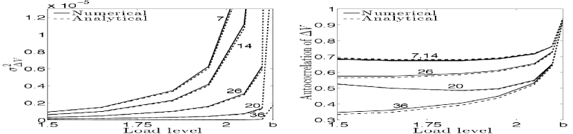
Figure 1: Variance and autocorrelation of voltage magnitudes for five buses in the 39-bus test case versus load level. Load level is the ratio of the system loads to their nominal values. b denotes the bifurcation point. The bus number associated with each curve is shown next to it. Here and everywhere below the autocorrelation time lag $t-s=0.2\textnormal{{s}}$.

By examining $\sigma^{2}$ and $R\left(\Delta t\right)$ for all buses in our test system, we have concluded that, as Fig. 1 illustrates, good EWS occur in two different types of buses. We found that $\sigma^{2}$ is a good EWS for load buses, whereas $R\left(\Delta t\right)$ is a good EWS at buses that are close to generators with low inertia. In addition, we found that $\sigma_{\Delta V}^{2}$ at generator buses is much smaller than at load buses, largely due to generator voltage control systems. As explained in Sec. IV, this limits the use of $R_{\Delta V}\left(\Delta t\right)$ at generator buses as an EWS.

III-B Autocorrelation and Variance of Line Currents

The fact that autocorrelation of voltages is not uniformly useful as an EWS prompted us to look at other variables, particularly currents, that might be more useful indicators. Results for $\sigma^{2}$ and $R\left(\Delta t\right)$ of currents, shown in Fig. 2, suggest that while $\sigma_{\Delta I}^{2}$ of almost all lines increase measurably with the increase of the load level, increased $R_{\Delta I}(\Delta t)$ is clearly observable only in some of the lines, such as line $\left[6\,\,31\right]$. As was the case with voltages, the common characteristic of lines that show clear increases in $R_{\Delta I}(\Delta t)$ is that they are connected to a generator with low or moderate inertia. The explanation for this appears to be that increased $R_{\Delta I}\left(\Delta t\right)$ is closely tied to the way that generators respond to perturbations as the system approaches bifurcation. Increases in $R_{\Delta I}(\Delta t)$ are not clearly observable in lines that are close to load centers, such as line $\left[4\,\,14\right]$ in Fig. 2.

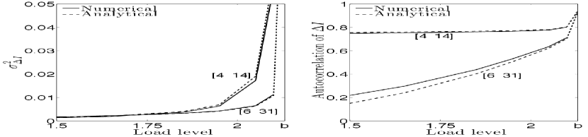
Figure 2: Variance and autocorrelation of current of two lines. The numbers in brackets are bus numbers at two ends of the lines.

Examining changes in $\sigma^{2},\,R\left(\Delta t\right)$ of several state variables showed that only magnitudes of voltages and line currents signal the proximity to the bifurcation well under certain conditions mentioned above. Other variables such as voltage angle, current angle, generator rotor angle and generator speed did not show measurable or clear monotonically increasing patterns in $\sigma^{2},\,R\left(\Delta t\right)$ that can indicate proximity to a bifurcation.

IV Detectability after measurement noise

This section examines the detectability of increases in $\sigma^{2}$ and $R\left(\Delta t\right)$ of voltages and currents given the presence of measurement noise. In addition, we present a method for reducing the impact of measurement noise using a band-pass filter.

IV-A Impact of Measurement Noise on Variance and Autocorrelation

Clearly, measurement noise will adversely impact the observability of increases in $\sigma^{2},\,R\left(\Delta t\right)$ of voltages and currents. In order to model this impact, we assumed that measurement noise at each bus is normally distributed with a standard deviation that is proportional to the steady-state mean voltage for this load level: $\sigma_{\eta}=0.01\left\langle V\right\rangle$. As a result the measured variance, $\sigma_{\Delta V_{m}}^{2}$, of a bus voltage increases to:

$$\sigma_{\Delta V_{m}}^{2}=\sigma_{\Delta V}^{2}+\sigma_{\eta}^{2}$$ (27)

where $\sigma_{\Delta V}^{2}$ is the variance before adding measurement noise.

Applying this method, Fig. 3 shows $\sigma^{2}$ and $R\left(\Delta t\right)$ for the voltage magnitudes of the same five buses used in Sec. III-A, but after adding measurement noise. The results show that measurement noise causes the increases in $\sigma_{\Delta V_{m}}^{2}$ to occur only close to the bifurcation, except for bus 36. In fact, $\sigma_{\Delta V_{m}}^{2}$ decreases for most buses, until close to the bifurcation. The reason for this decrease is that, based on (27), $\sigma_{\eta}^{2}$ decreases with $\left\langle V\right\rangle$, and $\left\langle V\right\rangle$ decreases as the system moves toward the nose of the PV curve. Also, because of the 1% measurement noise, $\sigma_{\eta}^{2}>\sigma_{\Delta V}^{2}$ until close to the bifurcation for most buses. For bus 36, which is a generator bus, $\sigma^{2}$ is almost constant since $\left\langle V\right\rangle$ (and as a result of $\sigma_{\eta}^{2}$) is held constant by the exciter; $\sigma_{\eta}^{2}\gg\sigma_{\Delta V}^{2}$ for generator buses.

Fig. 3 also shows that $R_{\Delta V_{m}}\left(\Delta t\right)$ increases significantly near the bifurcation for buses 7, 14 and, to a lesser extent, for bus 26. Appendix A demonstrates that the increase in $R_{\Delta V_{m}}\left(\Delta t\right)$ of these buses is largely an artifact of adding measurement noise: it is primarily due to increases in $\sigma^{2}$ rather than that of $R\left(\Delta t\right)$. Autocorrelation of $\Delta V_{m}$ is almost zero for buses 20, 36 since the uncorrelated measurement noise dominates the voltage of buses near generators.

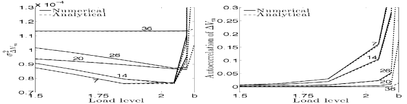
Figure 3: Variances and autocorrelations of voltage magnitudes of five buses in the 39-bus test case versus load level, accounting for measurement noise.

Thus, measurement noise essentially washes out the useful EWS that we reported in Sec. III-A. In addition, there is another issue impacting the detectability of EWS, which we discuss in the next subsection.

IV-B Spread of Statistics

One important point regarding the detection of increased $\sigma^{2}$ and $R\left(\Delta t\right)$ is that the measured statistics of a sample of a variable’s measurement data (which an operator can observe in finite time) are different from the mean statistical properties of that variable over infinitely many measurements. Although the mean of these statistics typically grows as the system approaches a bifurcation, the variance (spread) of these statistics that results from finite sample sizes can cause difficulty in estimating the distance to the bifurcation.

In order to quantify the detectability of an increase in $\sigma^{2}\,\textnormal{{or}}\,R\left(\Delta t\right)$, we introduce an index $q_{95/80}$ (see Fig. 4):

$$q_{95/80}=\int_{a}^{\infty}f_{X\left(80\%\right)}dx+\int_{-\infty}^{a}f_{X\left(95\%\right)}dx$$ (28)

where $X$ is the statistic of interest ($\sigma^{2}\,\textnormal{{or}}\,R\left(\Delta t\right)$), $f_{X\left(80\%\right)}\,\textnormal{{and}}\,f_{X\left(95\%\right)}$ are the probability density functions (pdfs) of $X$ for load levels of $80\%\,\textnormal{{and}}\,95\%$ of the bifurcation, and $a$ is the point where the two distributions intersect. This measure ranges from 0 to 1, where $0$ suggests that there is no overlap between the two distributions, such that detectability is unimpeded by the statistic’s spread, while $q_{95/80}=1$ means that the two distributions completely overlap—i.e. the statistic does not increase. When the statistic has a decreasing trend, we declare $q_{95/80}=NA$. $q_{95/80}$ roughly corresponds to the probability of being able to correctly distinguish between the measured statistics at 80% and 95% load levels.

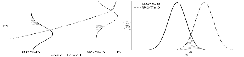
Figure 4: The left panel shows the empirical pdfs of $X$, which can be $\sigma^{2}\,\textnormal{{or}}\,R\left(\Delta t\right)$ of measurements for two load levels. Measure $q_{95/80}$ is equal to the sum of the hatched areas. The dash-dot line shows the mean of $X$ versus load level. The right panel shows an alternative view of the pdfs.

IV-C Filtering Measurement Noise

In this section, we explore the use of a band-pass filter to reduce the impact of measurement noise on the statistics of voltage and current measurements. The reason for filtering out the high frequency content of measurements is that the power spectral density (PSD) of voltages and currents (see Fig. 5) shows that the power of the system noise (i.e., voltage or current magnitude variations in response to load fluctuations) is concentrated mostly in its low frequencies. This appears to be typical for Hopf and saddle-node bifurcations in power systems. On the other hand, in order to detect CSD, it is necessary to remove slow trends that result not from CSD but from other factors, such as gradual changes in the system’s operating point [32]. By experimentation, we found that a band-pass filter with a pass-band of [0.1, 2] Hz reduces the impact of measurement noise in this system optimally. The rationale for these bounds can be seen from Fig. 5, which shows the PSD of a typical current magnitude in our system. We use this filter for all “filtered” results reported subsequently.

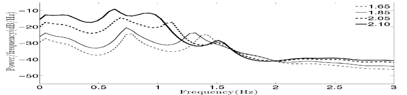
Figure 5: Power spectral density of the current of line [6 31] for several load levels listed in the legend. Bifurcation is at load level=2.12.

Fig. 6 shows $\sigma_{\Delta V}^{2},\,R_{\Delta V}\left(\Delta t\right)$ of buses 7, 36 after filtering measurement noise. Comparing Fig. 6 with Fig. 3 shows that using the band-pass filter significantly improves the detectability of increases in $\sigma_{\Delta V_{7}}^{2}$, which is close to load centers, but is not effective for bus 36, which is connected to a generator. The reason is that, even with filtering, it is still necessary that $\sigma^{2}$ without measurement noise be sufficiently large so that measurement noise does not dominate it. $\sigma^{2}$ of measurement noise after filtering will approximately be:

$$\sigma_{\eta f}^{2}=\sigma_{\eta}^{2}\cdot\nicefrac{{\left(f_{H}-f_{L}\right)}}{{\left(\nicefrac{{f_{s}}}{{2}}\right)}}$$ (29)

where $\sigma_{\eta f}^{2}$ is the variance of measurement noise after filtering; $f_{H},f_{L}$ are upper and lower cut-off frequencies of the filter; and $f_{s}$ is the sampling frequency of measurements. Assuming $\sigma_{\eta}^{2}=1e-4\,\textnormal{{and}}\,f_{s}=60\textnormal{{Hz}}$, we get $\sigma_{\eta f}^{2}=6.3\times 10^{-6}$. From Fig. 1, one can see that only $\sigma_{\Delta V}^{2}$ of the load buses exceeds this value near the bifurcation.

Fig. 6 also shows that after filtering out measurement noise, the increase in $R_{\Delta V_{7}}\left(\Delta t\right)$ is detectable near the bifurcation. However, as mentioned in Sec. IV-A, increases in $R(\Delta t)$ primarily result from increases in $\sigma_{\Delta V}^{2}$, and thus do not provide additional information regarding the proximity of the system to the bifurcation. Since $\sigma_{\eta}^{2}\gg\sigma_{\Delta V}^{2}$ for generator buses, $R_{\Delta V_{36}}\left(\Delta t\right)$ also does not increase measurably as the system approaches the bifurcation, even after filtering.

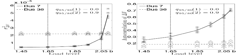
Figure 6: Variance and autocorrelation of voltage magnitude of buses 7,36 versus the load level after filtering the measurement noise. In this and subsequent figures, the lines show the mean and the discrete symbols $\left(*,\triangle\right)$ represent 5th, 25th, 75th, 95th percentiles of values of $\sigma^{2},\,R\left(\Delta t\right)$ for 100 realizations at each load level. The vertical dash-dot lines show $Load\,level=80\%b,\,95\%b$.

Similar to the case without measurement noise, $R\left(\Delta t\right)$ of line currents close to generators increase more clearly than that of lines near load centers. Fig. 7 shows $\sigma^{2},\,R\left(\Delta t\right)$ of currents of lines $\left[6\,\,31\right]$ and $\left[4\,\,14\right]$ after filtering the noise.

In general, filtering noise from line currents is easier than from voltages since the ratio of $\sigma^{2}$ of the system noise (defined above) to $\sigma^{2}$ of measurement noise is larger for currents.

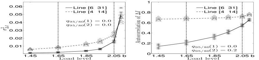
Figure 7: Variance and autocorrelation of currents of lines $\left[6\,\,31\right]$, $\left[4\,\,14\right]$ after filtering the measurement noise.

Fig. 8 shows the index $q_{95/80}$ for $\sigma_{\Delta V}^{2}$ across the 39-bus test case after filtering measurement noise. The results in Fig. 8 illustrate our earlier statement that $\sigma_{\Delta V}^{2}$ of buses near load centers are good EWS of the bifurcation while $\sigma_{\Delta V}^{2}$ of generator buses are not.

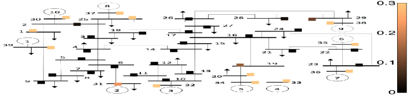
Figure 8: Index $q_{95/80}$ for $\sigma_{\Delta V}^{2}$ of bus voltages across the 39-bus test case. Here, and in Fig. 9, each rectangle represents the index $q_{95/80}$ for $\sigma_{\Delta V}^{2}$ of the bus next to it. In order to illustrate the results more clearly, we show $q_{95/80}=0.3$ for measurements with $q_{95/80}>0.3$, because quantities with this spread become indistinguishable.

Fig. 9 shows the index $q_{95/80}$ for $R_{\Delta I}\left(\Delta t\right)$ of lines across the 39-bus test case after filtering the measurement noise. The results in Fig. 9 show that $R_{\Delta I}\left(\Delta t\right)$ of the lines near generators provide good EWS of the bifurcation while $R_{\Delta I}\left(\Delta t\right)$ of the rest of the lines do not provide useful EWS.

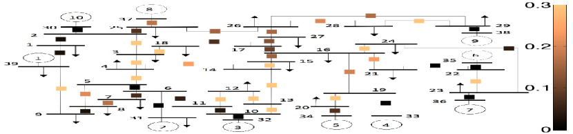
Figure 9: Index $q_{95/80}$ for $R_{\Delta I}\left(\Delta t\right)$ of lines across the 39-bus test case. Each rectangle represents index $q_{95/80}$ for $R_{\Delta I}\left(\Delta t\right)$ of the line next to it.

Note that while filtering of measurement noise can be helpful in detecting the increase in $\sigma_{\Delta V}^{2}$ of buses near load centers, it is not helpful in detecting an increase in $R_{\Delta V}\left(\Delta t\right)$ of these buses. This is because the $R_{\Delta V}\left(\Delta t\right)$ of such buses are not inherently good indicators of the proximity to the bifurcation; See Sec. III-A. Also, filtering measurement noise will not be helpful in retrieving the statistics of the bus voltages close to generators since their variances are small compared to that of measurement noise. On the contrary, $R_{\Delta I}\left(\Delta t\right)$ of lines near generators provide good EWS for the bifurcation, while $\sigma_{\Delta I}^{2}$ of almost all lines provide good EWS.

V Detecting Locations of Increased Stress

This section examines the potential to use statistical properties of measurements to detect the locations of increased stress in a power system. By studying two scenarios, we investigated whether patterns of change in $\sigma^{2}$ and $R\left(\Delta t\right)$ in a stressed area are different from the rest of the grid, so they can be helpful in identifying the location of the stressed area.

V-A Transmission line tripping

In the first scenario, we disconnected lines between buses 4, 14 and buses 4, 5 in order to increase stress in the area close to bus 4. For this experiment, the load level was held constant at 1.45 times the nominal. We calculated the ratio of $\sigma_{\Delta V}^{2}$ and $\sigma_{\Delta I}^{2}$ for the stressed case to the variances at the normal operating condition $\left(\textnormal{{Ratio}}\left(\sigma^{2}\right)\right)$. We also calculated the difference between $R_{\Delta V}\left(\Delta t\right)$ and $R_{\Delta I}\left(\Delta t\right)$ for the two cases $\left(\textnormal{{Diff}}\left(R\left(\Delta t\right)\right)\right)$. Values of $\textnormal{{Ratio}}\left(\sigma^{2}\right),\,\textnormal{{Diff}}\left(R\left(\Delta t\right)\right)$ that are sufficiently larger than 1 or 0 indicate significant increase in $\sigma^{2}$ or $R\left(\Delta t\right)$, respectively. Fig. 10(a) shows $\textnormal{{Ratio}}\left(\sigma_{\Delta V}^{2}\right)$ after adding measurement noise and filtering. The five bus voltages shown have the highest mean of $\textnormal{{Ratio}}\left(\sigma^{2}\right)$ among all buses. The figure shows that the voltage of the buses near bus 4 have the largest $\textnormal{{Ratio}}\left(\sigma_{\Delta V}^{2}\right)$ among the system buses. As with voltages, $\sigma_{\Delta I}^{2}$ close to bus 4 showed more growth than $\sigma_{\Delta I}^{2}$ in the rest of the system. These results suggest that larger increases in $\sigma_{\Delta V}^{2}$ and $\sigma_{\Delta I}^{2}$ in one area of the system, relative to the rest of the system, can indicate that this area is stressed.

Our results from Sec. IV identified certain lines whose autocorrelation of currents can be good EWS of bifurcation. We now comment on what behavior these autocorrelations exhibit in this experiment. It turns out that not all of these autocorrelations show a measurable increase; the five lines whose currents’ autocorrelations show the largest increases are shown in Fig. 10(b). While it is not possible to pinpoint the location of the disturbance based only on these statistical characteristics, it is possible to tell, based on the statistics, that the disturbance has occurred in a certain area of the network. This knowledge would reinforce the information obtained from monitoring variances of voltages and currents. As explained in Sec. IV-A, $R_{\Delta V}\left(\Delta t\right)$ does not provide useful information regarding which areas in the grid are most stressed.

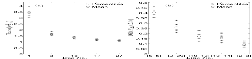
Figure 10: Panel (a) shows $\textnormal{{Ratio}}\left(\sigma_{\Delta V}^{2}\right)$ after disconnecting the two lines connected to bus 4. The mean of the $\textnormal{{Ratio}}\left(\sigma_{\Delta V}^{2}\right)$ for the 5 buses that show the highest increases in variance, as well as the 5th, 25th, 75th, 95th percentiles of their values, are shown. Panel (b) shows $\textnormal{{Diff}}\left(R_{\Delta I}\left(\Delta t\right)\right)$ for 5 lines that exhibit the largest increases in $R_{\Delta I}\left(\Delta t\right)$. The results are shown after filtering of measurement noise.

V-B Capacitor tripping

This section provides an example in which the statistical measures, $\sigma^{2}$ and $R\left(\Delta t\right)$, (at least partially) indicate the location of stress in the network, but the mean voltages $\left\langle V\right\rangle$ do not change enough to be good indicators. This example was designed to test the hypothesis that $\sigma^{2}$ and $R\left(\Delta t\right)$ can provide information that is not readily available from the mean values.

For this example, we added a new bus (bus 40) and an under-load tap changing (ULTC) transformer that connects bus 40 with bus 15. We also transferred the load of bus 15 to bus 40. Fig. 11 shows the P-V curve of bus 40 for three cases. In Case A, the system is in normal operating condition. In Case B, a 3-MVAR capacitor at bus 40 is disconnected and in Case C, the tap changer changes the tap from 1 to 1.1 in order to return the voltage to the normal operating range ($\left[0.95\,\,1.05\right]$ pu). Fig. 11 shows that the disconnection of the capacitor reduces the stability margin significantly, which manifests itself in lower voltage at bus 40. However, the increase in the ULTC’s tap ratio to 1.1 returns the voltage to a value close to its normal level.

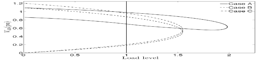
Figure 11: PV curve for the three cases described in Sec. V-B. The vertical line corresponds to the base load level.

Fig. 12(a) shows $\textnormal{{Ratio}}\left(\sigma_{\Delta I}^{2}\right)=\nicefrac{{{\sigma_{\Delta I,case\,C}^{2}}}}{{\sigma_{\Delta I,case\,A}^{2}}}$ for five lines, after filtering the measurement noise. These five line currents show the largest increase in $\sigma_{\Delta I}^{2}$ among all lines. The first three highest $\textnormal{{Ratio}}\left(\sigma_{\Delta I}^{2}\right)$ occur in lines that are close to the stressed area. However, some of the lines that are close to that area do not show significant or any increase in $\sigma_{\Delta I}^{2}$. For example, $\sigma_{\Delta I}^{2}$ of line $\left[\begin{array}[]{cc}14&15\end{array}\right]$ decreases. Nevertheless, considering lines with the highest growth in $\sigma_{\Delta I}^{2}$ can clearly be helpful in identifying the location of the area of the system under excessive stress. As was the case for line currents, the results show that buses that exhibit the largest increases in $\sigma_{\Delta V}^{2}$ are close to the stressed area. Fig. 12(b) shows $\textnormal{{Diff}}\left(R_{\Delta I}\left(\Delta t\right)\right)=R_{\Delta I,,case\,C}\left(\Delta t\right)-R_{\Delta I,,case\,A}\left(\Delta t\right)$ for 5 lines. The positive values indicate the increase in $R_{\Delta I}\left(\Delta t\right)$. The results in Fig. 12(b) show that lines that exhibit the largest increase in $R_{\Delta I}\left(\Delta t\right)$ are close to the stressed area.

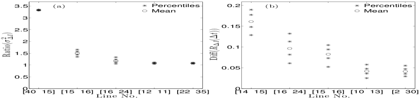
Figure 12: Panel (a) shows $\nicefrac{{{\sigma_{\Delta I,case\,C}^{2}}}}{{\sigma_{\Delta I,case\,A}^{2}}}$ for 5 lines that exhibit the largest increase in $\sigma_{\Delta I}^{2}$ among all lines. Panel (b) shows $R_{\Delta I,,case\,C}\left(\Delta t\right)-R_{\Delta I,,case\,A}\left(\Delta t\right)$ for 5 lines that exhibit the largest increase in $R_{\Delta I}\left(\Delta t\right)$.

V-C Discussion

The results presented in this section show that comparing $\sigma_{\Delta V}^{2}$ and $\sigma_{\Delta I}^{2}$ for a stressed operating condition with their variances for the normal operating condition can be useful in detecting stressed areas of a power system. The reason for this is that the variances of voltage and current magnitudes show larger increases near the stressed area of a power system, compared to variances in the rest of the system. The results also show that $R_{\Delta I}\left(\Delta t\right)$ can be helpful in detecting the stressed area’s approximate location, although it may not be helpful in pinpointing the exact location of the stress. Autocorrelation of bus voltages were not found to be useful for pinpointing the stressed location for the reason explained in Appendix A.

VI Conclusions

This paper investigates the use of statistical signals (autocorrelation and variance) in time-series data, such as what is produced from synchronized phasor measurement systems, as indicators of stability in a power system.

First, we derived a semi-analytical method for quickly computing the expected autocorrelation and variance for any voltage or current in a dynamic power system model. Computing the statistics in this way was shown to be orders of magnitude faster than obtaining the same result by simulation, and allows one to quickly identify locations and variables that are reliable indicators of proximity to instability. Using this method, we showed that the variance of voltage magnitudes near load centers, the autocorrelation of line currents near generators, and the variance of almost all line currents increased measurably as the 39-bus test case approached bifurcation. We found that these trends persist, even in the presence of measurement noise, provided that the data are band-pass filtered. Finally, the paper provides results suggesting that the statistics of voltage and current data can be helpful in identifying not only whether a system is seeing increased stress, but also the location of the stress.

Together, these results suggest that, under certain conditions, these easily measured statistical quantities in synchrophasor data can be useful indicators of stability.

Appendix A

The equation for $R_{\Delta V_{m}}\left(\Delta t\right)$ before band-pass filtering is:

$$\nicefrac{{\textnormal{E}\left[\Delta V_{m}\left(t\right)\Delta V_{m}\left(s\right)\right]}}{{\sigma_{\Delta V_{m}}^{2}}}=\nicefrac{{\textnormal{E}\left[\Delta V\left(t\right)\Delta V\left(s\right)\right]}}{{\left(\sigma_{\Delta V}^{2}+\sigma_{\eta}^{2}\right)}}$$ (30)

If $\sigma_{\Delta V}^{2}\ll\sigma_{\eta}^{2}$, $R_{\Delta V_{m}}\left(\Delta t\right)$ will be almost zero. This is the case for generator buses or buses close to generators such as buses $20,36$. However, if $\sigma_{\Delta V}^{2}$ increases such that $\sigma_{\Delta V}^{2}\sim\sigma_{\eta}^{2}$ and $R_{\Delta V}\left(\Delta t\right)$ is sufficiently larger than $0$ $\left(>0.2\right)$, then $R_{\Delta V_{m}}\left(\Delta t\right)$ will rise significantly with load level, in part because of increase in $R_{\Delta V}\left(\Delta t\right)$ and in part because of increase in $\sigma_{\Delta V}^{2}$. This happens for buses close to load centers such as $7,14$. Comparing $R\left(\Delta t\right)$ of voltage of buses $7,14$ in Fig. 1 with those in Fig. 3 shows that these quantities increase significantly after adding measurement noise while their increase without measurement noise is much smaller. This shows that the increase in $R_{\Delta V_{m}}\left(\Delta t\right)$ for load buses is more due to the increase in $\sigma_{\Delta V}^{2}$ than due to the increase in $R_{\Delta V}\left(\Delta t\right)$.

Author biographies

Goodarz Ghanavati (S‘11) received the B.S. and M.S. degrees in Electrical Engineering from Amirkabir University of Technology, Tehran, Iran in 2005 and 2008, respectively. Currently, he is pursuing the Ph.D. degree in Electrical Engineering at University of Vermont. His research interests include power system dynamics, PMU applications and smart grid.

Paul D. H. Hines (S‘96,M‘07,SM‘14) received the Ph.D. in Engineering and Public Policy from Carnegie Mellon University in 2007 and M.S. (2001) and B.S. (1997) degrees in Electrical Engineering from the University of Washington and Seattle Pacific University, respectively. He is currently an Associate Professor in the School of Engineering, with a secondary appointment in the Dept. of Computer Science, at the University of Vermont, and a member of the adjunct research faculty of the Carnegie Mellon Electricity Industry Center. Formerly he worked on various electricity industry projects at the U.S. National Energy Technology Laboratory, the US Federal Energy Regulatory Commission, Alstom ESCA, and Black and Veatch. He currently serves as the chair of the Green Mountain Section of the IEEE, as the vice-chair of the IEEE PES Working Group on Cascading Failure, and as an Associate Editor for the IEEE Transactions on Smart Grid.

Taras I. Lakoba received the Diploma in physics from Moscow State University, Moscow, Russia, in 1989, and the Ph.D. degree in applied mathematics from Clarkson University, Potsdam, NY, in 1996. His research interests include the effect of noise and nonlinearity in fiber-optic communication systems, stability of numerical methods, and perturbation techniques.

References

- [1] F. Alvarado, I. Dobson, and Y. Hu, “Computation of closest bifurcations in power systems,” IEEE Trans. Power Syst., vol. 9, no. 2, pp. 918–928, May 1994.
- [2] R. J. Avalos, C. A. Cañizares, F. Milano, and A. J. Conejo, “Equivalency of continuation and optimization methods to determine saddle-node and limit-induced bifurcations in power systems,” IEEE Trans. Circuits Syst. I, vol. 56, no. 1, pp. 210–223, Jan. 2009.
- [3] S. Grijalva, “Individual branch and path necessary conditions for saddle-node bifurcation voltage collapse,” IEEE Trans. Power Syst., vol. 27, no. 1, pp. 12–19, Feb. 2012.
- [4] M. Perninge, V. Knazkins, M. Amelin, and L. Soder, “Risk estimation of critical time to voltage instability induced by saddle-node bifurcation,” IEEE Trans. Power Syst., vol. 25, no. 3, pp. 1600–1610, Aug. 2010.
- [5] M. Haque, “On-line monitoring of maximum permissible loading of a power system within voltage stability limits,” IEE Proc. Gen. Trans. Dist., vol. 150, no. 1, pp. 107–112, Jan. 2003.
- [6] T. J. Browne, V. Vittal, G. T. Heydt, and A. R. Messina, “A comparative assessment of two techniques for modal identification from power system measurements,” IEEE Trans. Power Syst., vol. 23, no. 3, pp. 1408–1415, Aug. 2008.
- [7] I. Kamwa, A. K. Pradhan, and G. Joós, “Robust detection and analysis of power system oscillations using the Teager-Kaiser energy operator,” IEEE Trans. Power Syst., vol. 26, no. 1, pp. 323–333, Feb. 2011.
- [8] K. Wang and M. L. Crow, “The Fokker–Planck equation for power system stability probability density function evolution,” IEEE Trans. Power Syst., vol. 28, no. 3, pp. 2994–3001, Aug. 2013.
- [9] C. Nwankpa, S. Shahidehpour, and Z. Schuss, “A stochastic approach to small disturbance stability analysis,” IEEE Trans. Power Syst., vol. 7, no. 4, pp. 1519–1528, Nov. 1992.
- [10] P. M. Anderson and A. Bose, “A probabilistic approach to power system stability analysis,” IEEE Trans. Power Apparatus Syst., vol. PAS-102, no. 8, pp. 2430–2439, Aug. 1983.
- [11] E. Haesen, C. Bastiaensen, J. Driesen, and R. Belmans, “A probabilistic formulation of load margins in power systems with stochastic generation,” IEEE Trans. Power Syst., vol. 24, no. 2, pp. 951–958, May 2009.
- [12] S. Bu, W. Du, H. Wang, Z. Chen, L. Xiao, and H. Li, “Probabilistic analysis of small-signal stability of large-scale power systems as affected by penetration of wind generation,” IEEE Trans. Power Syst., vol. 27, no. 2, pp. 762–770, May 2012.
- [13] J. Munoz, C. Canizares, K. Bhattacharya, and A. Vaccaro, “An affine arithmetic-based method for voltage stability assessment of power systems with intermittent generation sources,” IEEE Trans. Power Syst., vol. 28, no. 4, pp. 4475–4487, Nov. 2013.
- [14] H. Huang, C. Chung, K. W. Chan, and H. Chen, “Quasi-Monte Carlo based probabilistic small signal stability analysis for power systems with plug-in electric vehicle and wind power integration,” IEEE Trans. Power Syst., vol. 28, no. 3, pp. 3335–3343, Aug. 2013.
- [15] M. Scheffer, J. Bascompte, W. A. Brock, V. Brovkin, S. R. Carpenter, V. Dakos, H. Held, E. H. Van Nes, M. Rietkerk, and G. Sugihara, “Early–warning signals for critical transitions,” Nature, vol. 461, no. 7260, pp. 53–59, 2009.
- [16] M. Scheffer, S. R. Carpenter, T. M. Lenton, J. Bascompte, W. Brock, V. Dakos, J. van de Koppel, I. A. van de Leemput, S. A. Levin, E. H. van Nes, M. Pascual, and J. Vandermeer, “Anticipating critical transitions,” Science, vol. 338, no. 6105, pp. 344–348, Oct. 2012.
- [17] H. Mori, “On the relaxation processes near the second order phase transition point,” Prog. Theor. Phys., vol. 30, no. 4, pp. 576–578, 1963.
- [18] M. C. Boerlijst, T. Oudman, and A. M. de Roos, “Catastrophic collapse can occur without early warning: examples of silent catastrophes in structured ecological models,” PLOS ONE, vol. 8, no. 4, pp. e62 033, 6 pp, 2013.
- [19] E. Cotilla-Sanchez, P. Hines, and C. Danforth, “Predicting critical transitions from time series synchrophasor data,” IEEE Trans. Smart Grid, vol. 3, no. 4, pp. 1832 –1840, Dec. 2012.
- [20] D. Podolsky and K. Turitsyn, “Random load fluctuations and collapse probability of a power system operating near codimension 1 saddle-node bifurcation,” in IEEE Power and Energy Soc. Gen. Meeting, Jul. 2013, pp. 1–5.
- [21] S. Dhople, Y. Chen, L. DeVille, and A. Dominguez-Garcia, “Analysis of power system dynamics subject to stochastic power injections,” IEEE Trans. Circ. Syst. I, vol. 60, no. 12, pp. 3341–3353, Dec. 2013.
- [22] G. Ghanavati, P. D. Hines, T. I. Lakoba, and E. Cotilla-Sanchez, “Understanding early indicators of critical transitions in power systems from autocorrelation functions,” IEEE Trans. Circuits Syst. I, vol. 61, no. 9, pp. 2747–2760, Sep. 2014.
- [23] B. Yuan, M. Zhou, G. Li, and X.-P. Zhang, “Stochastic small-signal stability of power systems with wind power generation,” IEEE Trans. Power Syst., to be published.
- [24] A. J. F. Hauer, D. J. Trudnowski, and J. G. DeSteese, “A perspective on WAMS analysis tools for tracking of oscillatory dynamics,” in IEEE Power and Energy Soc. General Meeting, Jun. 2007, pp. 1–10.
- [25] G. Berg, “Power system load representation,” in Proc. IEE, vol. 120, no. 3, Mar. 1973, pp. 344–348.
- [26] F. Milano, Power System Analysis Toolbox Quick Reference Manual for PSAT version 2.1. 6, May 2010.
- [27] M. Pai, Energy function analysis for power system stability, 1st ed. MA, USA: Kluwer Academic Publishers, 1989.
- [28] A. A. P. Lerm, C. A. Cañizares, and A. S. Silva, “Multiparameter bifurcation analysis of the South Brazilian power system,” IEEE Trans. Power Syst., vol. 18, no. 2, pp. 737–746, May 2003.
- [29] W. D. Rosehart and C. A. Cañizares, “Bifurcation analysis of various power system models,” Intl. J. Elec. Pow. Energy Syst., vol. 21, no. 3, pp. 171–182, Mar. 1999.
- [30] C. W. Gardiner, Stochastic Methods: A Handbook for the Natural and Social Sciences, 4th ed. Berlin, Germany: Springer, 2010.
- [31] F. Milano, “An open source power system analysis toolbox,” IEEE Trans. Power Syst., vol. 20, no. 3, pp. 1199–1206, 2005.
- [32] V. Dakos, M. Scheffer, E. H. van Nes, V. Brovkin, V. Petoukhov, and H. Held, “Slowing down as an early warning signal for abrupt climate change,” Proc. Natl. Acad. Sci., vol. 105, no. 38, pp. 14 308–14 312, Sep. 2008.
- [33] M. Chertkov, S. Backhaus, K. Turtisyn, V. Chernyak, and V. Lebedev, “Voltage collapse and ODE approach to power flows: Analysis of a feeder line with static disorder in consumption/production,” arXiv preprint arXiv:1106.5003, Jun. 2011.
- [34] A. Schellenberg, W. Rosehart, and J. A. Aguado, “Cumulant-based stochastic nonlinear programming for variance constrained voltage stability analysis of power systems,” IEEE Trans. Power Syst., vol. 21, no. 2, pp. 579–585, May 2006.
- [35] Y. Kataoka, “A probabilistic nodal loading model and worst case solutions for electric power system voltage stability assessment,” IEEE Trans. Power Syst., vol. 18, no. 4, pp. 1507–1514, Nov. 2003.
- [36] D. Podolsky and K. Turitsyn, “Critical slowing-down as indicator of approach to the loss of stability,” arXiv preprint:1307.4318, Jul. 2013.
- [37] G. Hou and V. Vittal, “Trajectory sensitivity based preventive control of voltage instability considering load uncertainties,” IEEE Trans. Power Syst., vol. 27, no. 4, pp. 2280–2288, Nov. 2012.
- [38] D. Wei and X. Luo, “Noise-induced chaos in single-machine infinite-bus power systems,” Europhys. Lett., vol. 86, no. 5, pp. 50 008, 6 pp, 2009.
- [39] H. Ghasemi and C. A. Cañizares, “Confidence intervals estimation in the identification of electromechanical modes from ambient noise,” IEEE Trans. Power Syst., vol. 23, no. 2, pp. 641–648, 2008.
- [40] M. Anghel, K. A. Werley, and A. E. Motter, “Stochastic model for power grid dynamics,” in 40th Annual Hawaii Intl. Conf. Syst. Sci., Jan. 2007.
- [41] H. Verdejo, L. Vargas, and W. Kliemann, “Stability of linear stochastic systems via Lyapunov exponents and applications to power systems,” Appl. Math. Comput., vol. 218, no. 22, pp. 11 021–11 032, Jul. 2012.
- [42] H. Huang and C. Chung, “Coordinated damping control design for DFIG-based wind generation considering power output variation,” IEEE Trans. Power Syst., vol. 27, no. 4, pp. 1916–1925, Nov. 2012.
- [43] T. Odun-Ayo and M. L. Crow, “Structure-preserved power system transient stability using stochastic energy functions,” IEEE Trans. Power Syst., vol. 27, no. 3, pp. 1450–1458, 2012.
- [44] P. Kundur, J. Paserba, V. Ajjarapu, G. Andersson, A. Bose, C. Canizares, N. Hatziargyriou, D. Hill, A. Stankovic, C. Taylor, T. Van Cutsem, and V. Vittal, “Definition and classification of power system stability IEEE/CIGRE joint task force on stability terms and definitions,” IEEE Trans. Power Syst., vol. 19, no. 3, pp. 1387 – 1401, Aug. 2004.
- [45] Z. Y. Dong, J. H. Zhao, and D. Hill, “Numerical simulation for stochastic transient stability assessment,” IEEE Trans. Power Syst., vol. 27, no. 4, pp. 1741–1749, Nov. 2012.
- [46] C. De Marco and A. Bergen, “A security measure for random load disturbances in nonlinear power system models,” IEEE Trans. Circuits Syst., vol. 34, no. 12, pp. 1546–1557, Dec. 1987.
- [47] J. M. Lim and C. L. DeMarco, “Model-free voltage stability assessments via singular value analysis of PMU data,” in Bulk Pow. Syst. Dyn. Cont.-IX Optim. Secu. Cont. Emer. Pow. Grid Symp., Aug. 2013, pp. 1–10.
- [48] N. Kakimoto, M. Sugumi, T. Makino, and K. Tomiyama, “Monitoring of interarea oscillation mode by synchronized phasor measurement,” IEEE Trans. Power Syst., vol. 21, no. 1, pp. 260–268, Feb. 2006.
- [49] K. Wang, C. Chung, C. Tse, and K. Tsang, “Improved probabilistic method for power system dynamic stability studies,” in IEE Proc. Gen. Trans. Dist., vol. 147, no. 1, Jan. 2000, pp. 37–43.
- [50] F. Milano and R. Zarate-Minano, “A systematic method to model power systems as stochastic differential algebraic equations,” IEEE Trans. Power Syst., vol. 28, no. 4, pp. 4537–4544, Nov. 2013.