Electron Heating During Magnetic Reconnection: A Simulation Scaling Study

Abstract

Electron bulk heating during magnetic reconnection with symmetric inflow conditions is examined using kinetic particle-in-cell (PIC) simulations. Inflowing plasma parameters are varied over a wide range of conditions, and the increase of electron temperature is measured in the exhaust well downstream of the x-line. The degree of electron heating is well correlated with the inflowing Alfvén speed $c_{Ar}$ based on the reconnecting magnetic field through the relation $\Delta T_{e}=0.033\,m_{i}\,c_{Ar}^{2}$, where $\Delta T_{e}$ is the increase in electron temperature. For the range of simulations performed, the heating shows almost no correlation with inflow total temperature $T_{tot}=T_{i}+T_{e}$ or plasma $\beta$. An out-of-plane (guide) magnetic field of similar magnitude to the reconnecting field does not affect the total heating, but it does quench perpendicular heating, with almost all heating being in the parallel direction. These results are qualitatively consistent with a recent statistical survey of electron heating in the dayside magnetopause (Phan et al, Geophys. Res. Lett., 40, doi:10.1002/grl.50917, 2013), which also found that $\Delta T_{e}$ was proportional to the inflowing Alfvén speed. The net electron heating varies very little with distance downstream of the x-line. The simulations show at most a very weak dependence of electron heating on the ion to electron mass ratio. In the antiparallel reconnection case, the largely parallel heating is eventually isotropized downstream due a scattering mechanism such as stochastic particle motion or instabilities. The simulation size is large enough to be directly relevant to reconnection in the Earth’s magnetosphere, and the present findings may prove to be universal in nature with applications to the solar wind, the solar corona, and other astrophysical plasmas. The study highlights key properties that must be satisfied by an electron heating mechanism: (1) Preferential heating in the parallel direction; (2) Heating proportional to $m_{i}\,c_{Ar}^{2}$; (3) At most a weak dependence on electron mass; and (4) An exhaust electron temperature that varies little with distance from the x-line.

I Introduction

Magnetic reconnection is a universal plasma process which converts stored magnetic energy into particle energy. The process is believed to be important in many astrophysical, solar, geophysical, and laboratory contexts. An important unresolved problem in reconnection research is to understand what controls electron energization in reconnection exhausts. Past investigations have explored suprathermal electron energization, both observationally [e.g., Ref. Baker and Stone, 1976; Hoshino et al., 2001; Oieroset et al., 2002; Chen et al., 2008; Retinò et al., 2008] and theoretically [e.g., Ref. Hoshino et al., 2001; Pritchett, 2006; Drake et al., 2006; Egedal et al., 2010]. However, an even more basic problem is the reconnection associated thermal heating of electrons. By thermal heating, we mean heating of the core population and not the energetic tail of the distribution. Space observations suggest that the degree of thermal heating depends on plasma parameters. Strong heating is typically observed in reconnection exhausts in Earth’s magnetotailAngelopoulos et al. (1992), while much weaker heating occurs in magnetopauseGosling et al. (2006); Phan et al. (2013) and solar wind exhaustsGosling et al. (2007); Pulupa et al. (2014).

These disparate space observations may be consistent with the heating being primarily controlled by inflow conditions. In a recent statistical observation studyPhan et al. (2013), the degree of electron bulk heating in asymmetric reconnection exhausts at the Earth’s magnetopause was best correlated with the asymmetric outflow velocityCassak and Shay (2007); Swisdak and Drake (2007) $C_{A-{\rm asymm}}^{2}$. A best fit to the data produced the empirical relation: $\Delta T_{e}=M_{Te}\;m_{i}\,C_{A-{\rm asymm}}^{2}$, where $M_{Te}$ is a constant with $M_{Te}=0.017,$ the “$\Delta$”refers to the change in temperature from the magnetosheath inflowing plasma and $T_{e}$ is related to the trace of the full electron temperature tensor ${\bf T}_{e}$ as $T_{e}={\rm Tr}\,[{\bf T}_{e}]/3$. The linear dependence of the heating indicates that the heating is proportional to the inflowing magnetic energy per proton-electron pair. It was also found in that study that perpendicular heating is substantially reduced in the presence of a strong guide field.

Simulation case studies have examined electron temperatures and distributions during reconnection, finding that heating and associated anisotropies can be generated due to many mechanisms such as acceleration in the reconnection electric field, turbulent waves excited by Hall electric currents, betatron acceleration, Fermi reflection on curved moving field lines, and trapped electron populations due to parallel electric fields [e.g., Ref. Horiuchi and Sato, 1997; Hoshino, Hiraide, and Mukai, 2001; Swisdak et al., 2005; Fujimoto and Machida, 2006; Drake et al., 2006; Chen et al., 2008; Le et al., 2009; Egedal, Daughton, and Le, 2012]. A more recent kinetic PIC simulation study found that the dominant energization mechanism was Fermi reflection for nearly antiparallel reconnection and both Fermi reflection and parallel electric fields for stronger guide fieldsDahlin, Drake, and Swisdak (2014). A laboratory analysis of reconnection found that electrons are primarily energized close to the x-line with this energy transferred into the exhaust via heat conductionYamada et al. (2014). In terms of theory and modeling, it is currently unclear how different reconnection conditions modify the magnitude of the electron heating and the heating mechanism. What is currently needed is a systematic simulation study of the degree of thermal electron heating in the exhaust region of magnetic reconnection and how it depends on a variety of inflow parameters. Such a study will directly test whether simulations can reproduce results consistent with observations, and will provide a testbed for determining the ultimate cause of the electron heating.

We perform a series of fully kinetic particle-in-cell simulations examining the scaling of the electron heating for a range of inflow conditions and parameters. In this initial study, we choose first to focus on the simpler case of symmetric reconnection, which will provide context when the more complicated asymmetric reconnection is examined at a later date. Even so, the key findings in terms of scaling with the inflow Alfvén speed $(\,\Delta T_{e}\propto\;m_{i}\,C_{A{\rm in}}^{2}\,)$ and the anisotropy of heating are remarkably similar to the asymmetric reconnection observationsPhan et al. (2013), suggesting that this scaling is generic to reconnection.

The results have the following implications for an electron heating mechanism: (1) Preferential heating in the parallel direction; (2) Heating proportional to $m_{i}\,c_{Ar}^{2}$, where $c_{Ar}$ is the inflow Alfvén speed based upon the reconnecting magnetic field; (3) At most a weak dependence on electron mass; and (4) An exhaust electron temperature that varies little with distance from the x-line.

The present paper is organized as follows. In Section II, the theoretical context for electron heating during magnetic reconnection is examined. Section III describes the numerical simulations in this study. Section IV gives an example simulation. Section V describes how the degree of electron heating is determined from the simulations. Section VI describes the scaling of the heating. Section VII examines the effect of electron to ion mass ratio on the heating. Section VIII is the discussion and conclusion section.

II Theory

In order to give context to the analysis of simulation data, we examine the heating using Sweet-Parker reconnection theory (a control volume analysis). For full generality, we first perform the analysis on asymmetric reconnection and then take the symmetric limit for application to this study. Our analysis is similar to previous Sweet-Parker analyses of asymmetric reconnection Cassak and Shay (2007); Birn et al. (2010).

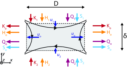
Figure 1: Schematic of the energy fluxes into and out of the diffusion region for asymmetric reconnection. Subscripts “1” and “2” denote different inflowing quantities, and subscript “o” denotes outflowing quantities. $u$ is bulk flow velocity, $K$ is bulk flow energy flux, $H$ is enthalpy flux, $Q$ is heat flux, and $S$ is electromagnetic Poynting flux. Adapted from [Eastwood et al., 2013]Eastwood et al. (2013).

Figure 1 shows a schematic of the energy fluxes into and out of the diffusion region. $u$ denotes bulk flow velocities. $\delta$ is the width of the outflow exhaust and $D$ is the width of the inflow region. $S$ is Poynting flux, $H$ is enthalpy flux, $K$ is bulk fluid kinetic energy flux, and $Q$ is heat flux. The inflowing conditions on the two sides have subscript “1” and “2,” and the outflowing quantities have subscript “o.” Conservation of energy requires:

$$D\;\left(S_{1}+S_{2}+H_{1}+H_{2}+K_{1}+K_{2}+Q_{1}+Q_{2}\right)\approx 2\,\delta\;\left(S_{o}+H_{o}+K_{o}+Q_{o}\right).$$ (1)

Ignoring the typically small incoming kinetic energy $K_{1}$ and $K_{2}$ and heat flux $Q_{1}$ and $Q_{2}$, this equation can be rewritten:

$$(S_{1}+S_{2})D\;\approx\;2\delta S_{o}+[\;2\delta H_{o}-D(H_{1}+H_{2})\;]\\ +2\delta K_{o}+2\delta Q_{o}.$$ (2)

Dividing by the incoming Poynting flux yields $1\approx R_{S}+R_{H}+R_{K}+R_{Q}$, where each $R$ term represents the fractional amount of energy (relative to the converted magnetic energy) which leaves the diffusion region as each energy type. This study is focused the amount of energy going into heating, which is directly related to the enthalpy flux leaving the diffusion region.

$$R_{H}=\frac{2\,\delta H_{o}-D(H_{1}+H_{2})}{D(S_{1}+S_{2})}.$$ (3)

This fractional enthalpy flux can be broken up into contributions from the ions and electrons as $R_{H}=R_{Hi}+R_{He}.$ For this study, we focus on the fractional electron enthalpy flux $R_{He}$ which is written using the definition of enthalpy as:

$$R_{He}=\frac{\Gamma\left[\;2\delta u_{o}P_{eo}-D(u_{1}P_{e1}+u_{2}P_{e2})\;\right]}{\frac{c}{4\pi}E_{z}(B_{1}+B_{2})D},$$ (4)

where $\Gamma\equiv\gamma/(\gamma-1)$, with $\gamma$ the ratio of specific heats. It is assumed that the inflowing $\Gamma$ is equal to the outflowing $\Gamma$, the applicability of which will be discussed in Section VIII. Note that we have written $S_{1}=(c/4\pi)\,E_{z}\,B_{1},$ with a similar relation for $S_{2}$. By doing so, we have discounted any Poynting flux associated with the out-of-plane (guide) magnetic field along $\hat{z}$. Because little $B_{z}$ energy is expected to be released in the diffusion region, this is a good approximation.

Using continuity, $2\delta\,n_{o}u_{o}\approx D\,(n_{1}u_{1}+n_{2}u_{2})$, along with $u_{1}=cE_{z}/B_{1}$ and $u_{2}=cE_{z}/B_{2}$, yields a relation for $R_{He}$:

$$R_{He}\approx\frac{\Gamma(T_{e0}-T_{ein})}{m_{i}u_{o}^{2}},$$ (5)

with the definitions:

$$T_{ein}=\frac{T_{e1}n_{1}B_{2}+T_{e2}n_{2}B_{1}}{n_{1}B_{2}+n_{2}B_{1}}$$ (6)

$$u_{o}^{2}=\frac{B_{1}B_{2}}{4\pi m_{i}}\;\frac{B_{1}+B_{2}}{n_{1}B_{2}+n_{2}B_{1}}$$ (7)

The form of $T_{ein}$ results from the fact that $T_{e1}$ and $T_{e2}$ are convected into the diffusion region with different velocities; it is the temperature of the outflowing plasma if there were only mixing and no heating. Therefore, to measure the actual change in thermal energy requires $T_{eo}-T_{ein}$. Note that $u_{o}$ is the outflow velocity for asymmetric reconnectionCassak and Shay (2007); Swisdak and Drake (2007).

$m_{i}\,u_{o}^{2}$ represents the available inflowing magnetic free energy per proton-electron pair, which can be shown by dividing the incoming Poynting flux by the inflowing particle density flux:

$$\frac{(S_{1}+S_{2})\,D}{(n_{1}u_{1}+n_{2}u_{2})\,D}=\frac{B_{1}B_{2}}{4\pi}\;\frac{B_{1}+B_{2}}{n_{1}B_{2}+n_{2}B_{1}}=m_{i}u_{0}^{2}$$ (8)

Note that the simulations in this study and observations of reconnection are not in thermodynamic equilibrium, with non-gaussian distribution functions and multiple beams. For that reason there is uncertainty as to the most appropriate value of $\Gamma$ to use for the outflowing plasma. We focus therefore simply on the ratio:

$$M_{Te}=\frac{T_{eo}-T_{ein}}{m_{i}u_{o}^{2}}.$$ (9)

$M_{Te}$ is a quantity that can be determined in a straightforward manner from each reconnection simulation, and is proportional to the amount of inflowing magnetic energy converted into electron heating. An important question regards the variation of $M_{Te}$ with changing inflowing parameters. It seems quite plausible that the percentage of magnetic energy converted to electron heating during magnetic reconnection would have a dependence on inflow conditions. If, on the other hand, $M_{Te}$ is a constant for a wide range of inflowing parameters, then the percentage of inflowing magnetic energy converted into electron heating is a constant.

In the symmetric reconnection limit, Eq. 9 simplifies to $M_{Te}=(T_{eo}-T_{ein})/(m_{i}c_{Ar}^{2})$, where $c_{Ar}$ is the Alfvén speed of the inflowing plasma based on the reconnecting magnetic field.

Another point to emphasize when studying the energy budget of reconnection regards the percentage of free energy converted to bulk outflows $R_{K}$. The Poynting flux of energy represents a “magnetic enthalpy” [e.g., Ref. Priest and Forbes, 2000]. and therefore contains twice the energy needed to accelerate the outflowing plasma to $u_{o}$, i.e., dividing outflow kinetic energy flux for a velocity $u_{o}$ by the incoming Poynting flux yields:

$$R_{K}=\frac{\left(\frac{1}{2}\,m_{i}\,n_{o}\,u_{o}^{3}\right)\;2\delta}{(S_{1}+S_{2})\,D}=\frac{1}{2}.$$ (10)

Even if 50% of the available inflowing magnetic energy is converted to bulk outflow energy, there will still be ample remaining magnetic energy to simultaneously heat the plasma.

III Simulation Information

We use the parallel PIC code P3DZeiler et al. (2002) to perform simulations in 2.5 dimensions of collisionless antiparallel reconnection. In the simulations, magnetic field strengths and particle number densities are normalized to arbitrary values $B_{0}$ and $n_{0}$, respectively. Lengths are normalized to the ion inertial length $d_{i0}=c/\omega_{pi0}$ at the reference density $n_{0}$. Time is normalized to the ion cyclotron time $\Omega_{ci0}^{-1}=(eB_{0}/m_{i}c)^{-1}.$ Speeds are normalized to the Alfvén speed $c_{A0}=\sqrt{B_{0}^{2}/(4\pi\,m_{i}\,n_{0})}$. Electric fields and temperatures are normalized to $E_{0}=c_{A0}B_{0}/c$ and $T_{0}=m_{i}c_{A0}^{2}$, respectively. The coordinate system is a generic “simulation coordinates,” meaning that the reconnection outflows are along $\hat{x}$ and the inflows are along $\hat{y}$, as illustrated in Figure 1.

Simulations are performed in a periodic domain with size and grid scale varied based on simulation and inflow parameters; upstream densities of n = 1.0, 0.2 and 0.04 have $L_{x}\times L_{y}=204.8\times 102.4,\;204.8\times 102.4,$ and $409.6\times 204.8$ respectively. There are three mass ratios $m_{i}/m_{e}=25,100,400,$ with grid scales $\Delta_{x}=\Delta_{y}=0.05,\,0.025,\,0.0125$ and speed of light $c=15,\,30,\,\ 40$ respectively. The initial conditions are a double current sheetShay, Drake, and Swisdak (2007). A small magnetic perturbation is used to initiate reconnection. Each simulation is evolved until reconnection reaches a steady state, and then during the steady-state period the simulation data is time averaged over 100 particle time steps, which is typically on the order of 50 electron plasma wave periods $\omega_{pe}^{-1}$.

In order to examine the effect of inflowing plasma conditions on electron heating, the initial simulation inflow parameters are varied over a range of values shown in Table 1. Variations in parameters are: reconnecting magnetic field Br between $1/\sqrt{5}$ and $\sqrt{5}$, density $n_{in}$ between 0.04 and 1.0, inflowing electron temperature $T_{e}$ between 0.03 and 1.25, and $T_{i}/T_{e}$ between 1 and 9. Simulations have either no guide field (anti-parallel reconnection) or a guide field $B_{g}=B_{r}$ (magnetic shear angle of $90^{\circ}$). The initial upstream reconnection Alfvén speed has values $c_{Ar}^{2}\equiv B_{r}^{2}/n_{in}=1.0,\;5.0,\;17.0,\;{\rm and}\;25.0$. The plasma total $\beta$ ranges from 0.06 to 5.0.

Note that for the purpose of connection with the Phan et al., 2013 magnetosheath inflow conditionsPhan et al. (2013), many of the $\beta$ values are substantially larger than typically used in generic kinetic PIC simulation studies. For example, the GEM challenge studyBirn et al. (2001) had inflow $\beta=0.2.$

IV Simulation Example

An overview of the reconnecting system is shown for run 46 in Figure 2: (a) $V_{ez}$ and (b) $V_{ex}$ with magnetic field lines, (c) $B_{z}$, (d) $T_{e||}$, (e) $T_{e\perp}$, and (f) $T_{e}=(T_{e||}+2\,T_{e\perp})/3$. Note that plots (d), (e), and (f) are on the same color scale to facilitate comparison. The out-of-plane electron flow is typical for anti-parallel reconnection, with flows near the x-line comparable to the electron Alfvén speed, and weaker flows near the separatrices and downstream of the x-line. The electron outflow shows the super-Alfvénic electron jets associated with the outer electron diffusion regionShay, Drake, and Swisdak (2007); Karimabadi, Daughton, and Scudder (2007), as well as the parallel electron flows near the separatrices associated with Hall currents. The out-of-plane magnetic field has the typical quadrupolar structure.

The heating of the electrons is evident in Figure 2d-f. There is strong electron parallel heating in the exhaust of the reconnection region. The perpendicular heating is localized very close to the midplane near the x-line but broadens to include the whole exhaust region downstream. In terms of the electron heating, we define the “near exhaust” $(45\lesssim x\lesssim 75)$ as the region with little perpendicular heating away from the midplane, and the “far exhaust” $\left[\,(25\lesssim x\lesssim 45)\;\;{\rm and}\;\;(75\lesssim x\lesssim 90)\,\right]$ as the regions downstream of that but before the edge of the reconnection jet front (in the past called the “dipolarization front”). The near exhaust is therefore associated with strong electron temperature anisotropy, while the temperature is more isotropic in the far exhaust.

A striking property of the heating in Figure 2f is that both the near and far exhausts are characterized by a nearly constant $T_{e}$. The constancy of $T_{e}$ with distance downstream of the x-line implies that electrons are continually being heated in the exhaust, with heating being just enough to bring the inflowing unheated plasma up to the exhaust temperature. The lack of perpendicular heating in the near exhaust implies that the heating mechanism first heats electrons along the parallel direction, with this parallel energy later being scattered into the perpendicular direction.

V Determination of Heating

We determine the downstream heating by examining a slice along $y$ in the exhaust at the following downstream distances: (1) $n_{in}$ = 0.2, distance = $20\,d_{i0}$, (2) $n_{in}$ = 1.0, distance = $9\,d_{i0}$, and (3) $n_{in}$ = 0.04, distance = $45\,d_{i0}.$ Normalized to the ion inertial length in the inflow region, these distances are all the same. All data used in the analysis of electron heating has been time averaged over 100 time steps, which is typically about 50 electron plasma wave periods $\omega_{pe}^{-1}$.

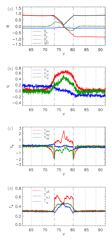
Figure 3: Determination of electron heating. Slices taken at $x=76.0125$ in Figure 2. (a) Magnetic fields, (b) Ion flow velocities, (c) Electron flow velocities, (d) Electron temperatures. Dashed vertical lines show exhaust region and dotted vertical lines show inflow regions.

Figure 3 shows slices of data along $y$ for the simulation described in Figure 2: (a) Magnetic fields, (b) Ion flows, (c) Electron Flows, (d) Electron Temperature, which shows typical exhaust properties for this type of reconnection. In (a) the quadrupolar Hall magnetic fields are evident, filling most of the exhaust region. In (b), the ion exhaust region is evident in red. Electron flows in the $x$ direction in red (c) show the super-Alfvénic electron outflows as well as the parallel flows towards the x-line near the separatrices. Plots of $T_{e},\,T_{e||},$ and $T_{e\perp}$ are shown in (d). There is a sharp drop of $T_{e||}$ and a sharp rise of $T_{e\perp}$ near the midplane, while $T_{e}$ stays relatively constant. Evidently, the electron thermal energy is simply being transferred between the perpendicular and parallel directions.

To determine the heating occurring in the outflow exhaust, we calculate the spatial average of the temperature in the exhaust $\overline{T_{e}}$, and subtract the average inflow temperature $T_{ein}$, yielding $\Delta T_{e}=\overline{T_{e}}-T_{eup}$. We calculate the anisotropic heating $\Delta T_{e||},\,\Delta T_{e\perp}$, and the total electron heating $\Delta T_{e}=(\Delta T_{e||}+2\,\Delta T_{e\perp})/3$. For Figure 3, the two upstream regions which determine the inflow values are shown with the vertical dotted lines. The exhaust region boundaries in this case are shown by the vertical dashed lines. In addition, the standard deviation of the temperature in the exhaust region is determined.

VI Scaling of Heating

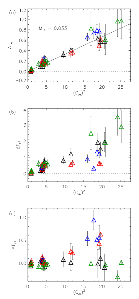
Figure 4: (a) $\Delta\,T_{e}$, (b) $\Delta\,T_{e||}$, and (c) $\Delta\,T_{e\perp}$ versus $c_{Ar}^{2}$ . Standard deviations of the averaging shown as error bars. Color of symbol represents type of run: (green) $m_{i}/m_{e}=25$ with guide field; (blue) $m_{i}/m_{e}=25$, antiparallel, $\beta<0.6;$ (black) $m_{i}/m_{e}=25$, antiparallel, $\beta\geq 0.6;$ (red) $m_{i}/m_{e}=100.$

The scaling of the heating for 56 simulations is shown in Figure 4: (a) $\Delta\,T_{e}$, (b) $\Delta\,T_{e||}$, and (c) $\Delta\,T_{e\perp}$ versus $c_{Ar}^{2},$ where $c_{Ar}$ is the Alfvén speed (using the reconnecting magnetic field) based upon the average upstream conditions determined from each run (as shown in Figure 3d). The colors of the symbols represent some important properties of each run: (green) $m_{i}/m_{e}=25$ with guide field; (blue) $m_{i}/m_{e}=25$, antiparallel, $\beta<0.6;$ (black) $m_{i}/m_{e}=25$, antiparallel, $\beta\geq 0.6;$ (red) $m_{i}/m_{e}=100.$ The standard deviations of the temperature are shown as error bars for each data point.

As discussed in Section II, for each simulation the percentage of magnetic energy converted to electron heating is proportional to: $M_{Te}=\Delta T_{e}/(m_{i}\,c_{Ar}^{2})$. In Figure 4a, $\Delta T_{e}$ for each simulation is plotted versus $m_{i}c_{Ar}^{2}$. The data roughly follows a straight line, meaning that the percentage of magnetic energy converted into electron heating is approximately constant across the simulations. The best fit line through the origin, fitting $\Delta T_{e}=M_{Te}\,c_{Ar}^{2}$, yields $M_{Te}=0.033,$ which is about twice the slope from Phan et al., 2013. What is striking is the universality of the scaling of electron temperature, independent of guide field and $\beta$, which vary considerably over the 56 runs.

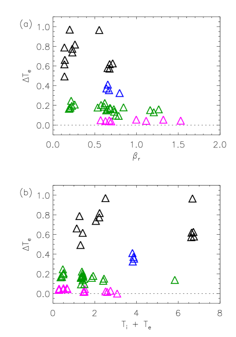
Figure 5: Electron heating versus (a) $\beta_{r}$ and (b) $T_{tot}=T_{i}+T_{e}.$ $\beta_{r}$ and $T_{tot}$ are determined using the average values upstream when the electron heating is determined, as is described in Figure 3. The color of the symbol refers to the asymptotic Alfvén speed in the upstream region using the asymptotic reconnecting field and density shown in Table 1: (black) $c_{Ar}^{2}=25;$ (blue) $c_{Ar}^{2}=14;$ (green) $c_{Ar}^{2}=5;$ and (magenta) $c_{Ar}^{2}=1.$

To verify that parameters such as $\beta$ and temperature are not playing a primary role in determining the heating, in Figure 5 we plot the dependence of electron heating on the inflowing values of (a) $\beta_{r}$ and (b) $T_{tot}=T_{i}+T_{e}.$ $\beta_{r}$ is determined using the reconnecting magnetic field component. Care must be taken in analyzing the results because the simulation space does not fill in all of parameter space. We therefore organize the data points by the asymptotic upstream Alfvén speed: (black) $c_{Ar}^{2}=25;$ (blue) $c_{Ar}^{2}=14;$ (green) $c_{Ar}^{2}=5;$ and (magenta) $c_{Ar}^{2}=1.$ It may appear that there is some heating dependence on $\beta_{r}$, with less heating for higher $\beta_{r}$. However, the color coding makes it clear that this dependence is likely due to the dearth of high $\beta_{r}$ with high Alfvén speed simulations, which are computationally challenging to perform. It is clear that any affect on heating from $\beta_{r}$ and $T_{tot}$ plays at most a secondary role to the upstream Alfvén speed.

A different story emerges from the scaling of $\Delta T_{e||}$ and $\Delta T_{e\perp}$ because the spatial structure of the anisotropy depends on $\beta$. Examining heating in the exhaust at a fixed distance from the x-line leads to different measured anisotropies. Figure 4b and 4c show the parallel and perpendicular heating, respectively. Focussing first on the guide field cases written as green points, it is striking that there is no perpendicular heating in these cases. A surprise, however, is that several of the anti-parallel simulations exhibit this anisotropy also, with little or no perpendicular heating. The reason to separate the $m_{i}/m_{e}=25$ cases into high $\beta$ and low $\beta$ becomes clear in Figures 4b and 4c. For the high $c_{Ar}$ cases, the guide field (green symbols) and the black symbols (higher $\beta$) show no perpendicular heating and greater parallel heating. This points to a faster isotropization closer to the x-line for the lower $\beta$ simulations with $m_{i}/m_{e}=25$ as well as all of the $m_{i}/m_{e}=100$ cases.

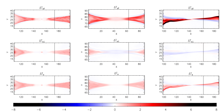
Figure 6: Change in temperature relative to upstream value for three different runs highlighting the change in the character of the heating for the change in $\beta$ and the change in guide field. All runs have $m_{i}/m_{e}=25.$ (left) run 25 with no guide field and $\beta=0.12;$ (middle) run 33 with no guide field and $\beta=0.6;$ (right) run 45 with guide field equal reconnecting field and $\beta=0.3.$

Figure 6 shows this difference in isotropization in more detail, where the the change in electron temperature from the upstream values are shown for $m_{i}/m_{e}=25$ cases with varying $\beta$ and guide field: (left) run 25 with no guide field and $\beta=0.12;$ (middle) run 33 with no guide field and $\beta=0.6;$ (right) run 45 with guide field equal reconnecting field and $\beta=0.3.$ The vertical line in the figure shows for each run where the vertical slice was taken to determine the heating.

Focussing on the anti-parallel cases first (left and middle columns), both show exhaust-filling total electron heating $\Delta T_{e}$ which onsets about $10\,d_{i0}$ downstream of the x-line. As with run 46 in Figure 2, this average $\Delta T_{e}$ is relatively uniform beyond $10\,d_{i0}.$ Note that the leftmost simulation has just started to develop a secondary island. For both $\beta$ values the onset of parallel heating occurs closer to the x-line than the perpendicular heating. However, for the lower $\beta$ case, $\Delta T_{e\perp}$ becomes exhaust filling perhaps $20\,d_{i0}$ downstream, whereas for the higher $\beta$ case this does not occur until around $30\,d_{i0}$ downstream. The lower $\beta$ case is isotropizing faster than the higher $\beta$ case.

The reason for this behavior is that lower $\beta$ cases exhibit stronger electron beaming relative to the electron thermal velocity and thus are much more susceptible to two-stream instabilities and electron hole formationCattell et al. (2005). In Figure 6, these instabilities are apparent in $\Delta T_{e||}$ for the low $\beta$ case as spatial fluctuations which onset simultaneously with the heating about $10\,d_{i0}$ downstream of the x-line. In contrast, the higher $\beta$ case has a much smoother $\Delta T_{e||}$, until around $x=75\,d_{i0},$ where oscillations become apparent. These may be due to a firehose-type instability, which isotropizes the electron temperature.

The guide field case is fundamentally different from the anti-parallel cases. The heating in the exhaust is strongly asymmetric along the normal direction (along $y$), and there is almost no $\Delta T_{e\perp}.$ These findings provide evidence that the heating mechanism or mechanisms first heat the electrons along the parallel direction which then scatters into the perpendicular direction.

VII Mass Ratio Dependence of Heating

An important question regards whether there is a mass dependence on the electron heating, as a realistic mass ratio is beyond the current supercomputer capabilities for a large scale statistical study such as this. Clearly, from Figure 4a, any mass ratio dependence is weak. The $m_{i}/m_{e}=100$ cases do have slightly lower heating for the highest $c_{Ar}$ values, but the difference is small.

To put this difference on a more numerical basis, we compare $M_{Te}$ for two different mass ratios. To make the comparison as straightforward as possible, we only compare simulations that have the same initial density, temperatures, and magnetic fields; these runs have a check mark in the “$m_{i}/m_{e}$ compare” column in Table 1. Figure 7 shows $\Delta T_{e}$ versus $m_{i}\,c_{Ar}^{2}$ for (a) $m_{i}/m_{e}=25$ and (b) $m_{i}/m_{e}=100.$ The coloring of data points uses the same convention as in Figure 4. There is a $\approx 10\%$ difference in $M_{Te}$ for the two mass ratios.

To provide a tentative scaling of heating versus mass ratio, we plot $M_{Te}$ versus $m_{i}/m_{e}$ in Figure 7c and calculate the best fit curve with the functional form $A\>(m_{i}/m_{e\\ })^{\alpha}$. Note that the $m_{i}/m_{e}=400$ case is a single simulation, run 56. A power law dependence with $A=0.055$ and $\alpha=-0.13$ is found, which as expected is a very weak dependence on mass ratio.

Extending this fit to a realistic mass ratio of $m_{i}/m_{e}=1836,$ we find $M_{Te}=0.020.$ This value is much closer to the experimental value from Phan et al., 2013 of 0.017, which is plotted as an asterisk in Figure 7. Thus, this weak mass ratio dependence is one possible explanation for the difference between the magnetopause observations findings and this simulation study.

VIII Discussion and Conclusions

A systematic kinetic-PIC simulation study of the effect of inflow parameters on the electron heating due to magnetic reconnection has been performed.We find that electron heating is well characterized by the inflowing Alfvén speed through the relation $\Delta T_{e}=M_{Te}\;m_{i}c_{Ar}^{2}$, where $M_{Te}$ is a constant of 0.033. For the range of inflow parameters performed, the heating shows almost no correlation with total temperature $T_{tot}=T_{i}+T_{e}$ or plasma $\beta$. A guide field of similar magnitude to the reconnecting field quenches perpendicular heating, with almost all heating being in the parallel direction. These findings are qualitatively consistent with a recent observational study of electron heatingPhan et al. (2013), which also found that $\Delta T_{e}$ was proportional to the inflowing Alfvén speed. A significant point regarding the simulation/observation comparison is that the observational study examined asymmetric inflow conditions while the simulations were of symmetric reconnection. Such an agreement implies that there may be a generic heating mechanism at work, and makes a case for the universality of the results of this study and the observational study.

An important question regarding magnetic reconnection is the ultimate fate of the released magnetic energy, i.e., the determination of the $R$ values described in Section II. MHD theory predicts that significant amounts of the released magnetic energy is converted to thermal energy, even in the incompressible limitBirn et al. (2010). The percentage of inflowing Poynting flux converted into electron enthalpy flux is given as $R_{He}=\Gamma\;\Delta T_{e}\,/\,(m_{i}c_{Ar}^{2})$, as reviewed in Section II. For an isotropic plasma, the average $M_{Te}=0.033$ in this study corresponds to the following percentage of inflowing Poynting flux converted to electron enthalpy flux: $R_{He}=5/2\,(0.033)=0.083$ or 8.3%. The Phan et al., 2013 observations give $R_{He}=5/2\,(0.017)\approx 0.043$, or 4.3%.

There is uncertainty in these percentages because both observations and kinetic PIC simulations exhibit temperature anisotropy in the exhaust (in the simulations the inflowing plasma is nearly isotropic). In a kinetic plasma with a pressure tensor ${\bf P}$, the general form for the “kinetic” enthalpy flux is ${\bf H}_{k}=(3/2)\,{\bf u}\,P+{\bf u}\cdot{\bf P}$, where $P\equiv{\rm Tr}[{\bf P}]\,/\,3$. If $T_{e||}\gg T_{e\perp},$ for example, the enthalpy flux along the magnetic field line would be 9/5 larger than the isotropic enthalpy flux, while the flux perpendicular to the field line would be 3/5 of the isotropic case. However, a preliminary analysis was performed examining both antiparallel and guide field cases in this study, and it was found that the integrated kinetic enthalpy flux across the exhaust was nearly equal to the predicted isotropic enthalpy flux.

The primary quantitative difference between this study and the observations is the value of $M_{Te}$, which for the simulations is approximately twice the value of the observations. The simulations do show a weak dependence on the electron mass with $\Delta T_{e}\approx 0.055\,(m_{i}/m_{e})^{-0.13}$, which when extrapolated to a realistic mass ratio gives $M_{Te}\approx 0.020,$ which is quite close to the $M_{Te}=0.017$ seen in the magnetopause observationsPhan et al. (2013). This would suggest that $M_{Te}$ is truly a universal feature, as the reconnection observations were for asymmetric reconnection, while these simulations are symmetric. While this finding is interesting, there are significant uncertainties as to the mass ratio scaling, as well as many other possible explanations for the quantitative difference between simulations and observations: 2D versus 3D, symmetric versus asymmetric, and observational uncertainties such as distance from the x-line, to name a few.

The relatively small electron enthalpy percentages for the simulations and observations are consistent with the outoing flux of energy being dominated by ion enthalpy flux, as seen in hybrid simulationsAunai, Belmont, and Smets (2011) and satellite observations in the Earth’s magnetotailEastwood et al. (2013). A recent laboratory studyYamada et al. (2014) of reconnection found that a magnetic energy inflow rate of $1.9\pm 0.2\,\text{MW}$ resulted in a change of electron thermal energy of $0.26\pm 0.1\,\text{MW}$, which represents a conversion rate of around 14%. However, comparison of this percentage with our simulation results is complicated because some aspects of the analysis methods for the laboratory study and our simulation study are different. For example, unlike our quasi-steady analysis, the laboratory experiment showed significant time dependence which was included in the energy conversion rate.

In all simulations, the heating in the exhaust region near the x-line is initially only in the parallel direction. For some cases, this parallel heating ultimately isotropizes at distances farther from the x-line. This finding implies that the heating mechanism primarily heats the plasma parallel to the magnetic field.

The isotropization of the parallel electron heating during antiparallel reconnection shows significant dependence on the upstream temperature and $\beta.$ At lower $\beta,$ streaming instabilities are stronger and thus the isotropization occurs closer to the x-line than for the higher $\beta$ cases.

A striking clue to the nature of the electron heating is that in the outflow exhaust $T_{e}$ shows little variation with distance from the x-line. Because cold inflowing electrons are continually ejected into the exhaust, this implies that electrons are being continually heated even far from the x-line.

Although the mechanism for electron heating is uncertain at this point, the findings in this study constrain the possible mechanisms: (1) Heating proportional to $m_{i}c_{Ar}^{2}$; (2) An exhaust electron temperature that varies little with distance from the x-line; (3) A preferential heating in the parallel direction, and (4) At most a very weak dependence on electron mass on the order of $(m_{i}/m_{e})^{-0.13}.$ The parallel heating rules out betatron acceleration because it would preferentially heat the plasma along the perpendicular direction [e.g., Ref. Birn et al., 2000]. There exists a parallel potential in the exhaust regionEgedal, Le, and Daughton (2013), which could lead to parallel heating through the generation of counterstreaming beams. On the other hand, Fermi-bounce heating through contracting magnetic field linesDrake et al. (2006); Dahlin, Drake, and Swisdak (2014) also produces preferential parallel heating. A recent kinetic-PIC studyDahlin, Drake, and Swisdak (2014) which found that electron energization was dominated by the Fermi reflection termDrake et al. (2006) for nearly anti-parallel reconnection, and by parallel electric fields and the Fermi mechanism in guide field reconnection. The physical mechanism of the electron heating mechanism will be a topic of a future study.

Energization and heating occurs naturally both at the x-line (e.g., Ref. Pritchett, 2006 and references therein) and in the flux pile-up region at the edge of the exhaustHoshino et al. (2001). Electrons that travel close enough to the x-line to demagnetize can be accelerated along the reconnection electric field, causing heating and energization. In Figure 2, the width of this electron demagnetization region is a few $d_{i0}$ along $x$. With a reconnection rate $E_{z}\approx 0.12$ and with the change in flux from the x-line to the edge of the electron demagnetization region being about 0.04, it takes a magnetic field line a time of about 0.4 to reconnect and travel to the edge of this region. Electrons that can propagate along a field line and enter this region during this time will be free accelerated to high velocities. With an upstream thermal velocity of around 7.0, only electrons within around $3\,d_{i0}$ from this region will be free accelerated. Therefore, the large majority of electrons in the simulation do not sample this inner region. If heating were only occurring very near the x-line, the electron temperature would be expected to decrease with distance from the x-line.

Regarding electron energization in the flux pileup region at the edge of the ion outflow exhaust, that region is transient in nature and is pushed downstream as the simulation progresses. In Figure 2, that region is around $30\,d_{i0}$ downstream of the x-line. This heating study does not examine electrons that have passed through the flux pileup region.

The applicability of this study for reconnection in physical systems is an important question, i.e., are the mechanisms of electron heating in the simulations likely to be similar to those found in actual physical systems? First, the consistency of these simulation results to the Phan et al., 2013 study is evidence for the relevance of the simulations. The findings of this study have been tested over a range of inflow conditions and ion to electron mass ratios. System size also plays an important role in the simulation relevance. While the simulations in this study are of sizes large enough to be applicable to reconnection in the magnetosphere, they are extremely small relative to distances in the solar wind and on the sun. However, the constancy of $T_{e}$ with distance from the x-line in the simulations gives some credence to the idea that the simulation heating mechanism has converged with system size.

Run	$m_{i}/m_{e}$ compare	$m_{i}/m_{e}$	$B_{r}$	$B_{g}$	$n_{in}$	$T_{e}$	$T_{i}$	Reference Number
1		25	1.000	0.000	0.20	0.250	0.250	301
2		25	1.000	1.000	0.20	0.250	0.250	302
3		25	1.000	0.000	0.20	0.250	2.250	303
4		25	1.000	1.000	0.20	0.250	2.250	304
5		25	1.000	0.000	1.00	0.250	0.250	307
6		25	1.000	1.000	1.00	0.250	0.250	311
7		25	0.447	0.000	0.20	0.250	0.250	308001
8		25	0.447	0.447	0.20	0.250	0.250	312001
9		25	1.000	0.000	0.04	0.250	2.250	309
10		25	1.000	1.000	0.04	0.250	2.250	313
11		25	2.236	0.000	0.20	0.250	2.250	310001
12		25	2.236	2.236	0.20	0.250	2.250	314001
13		25	0.447	0.000	0.20	0.250	2.250	319
14		25	0.447	0.447	0.20	0.250	2.250	320
15		25	1.000	0.000	1.00	0.250	2.250	321
16		25	1.000	1.000	1.00	0.250	2.250	322
17		25	1.000	0.000	0.20	0.250	1.250	323
18		25	1.000	1.000	0.20	0.250	1.250	324
19	$\checkmark$	25	1.000	0.000	0.20	0.063	0.313	325
20	$\checkmark$	25	1.000	1.000	0.20	0.063	0.313	326
21		25	1.000	1.000	0.20	1.000	5.000	328
22	$\checkmark$	25	1.000	0.000	0.20	0.250	1.250	601
23	$\checkmark$	25	1.000	1.000	0.20	0.250	1.250	604
24	$\checkmark$	25	0.447	0.000	0.20	0.250	1.250	602
25	$\checkmark$	25	2.236	0.000	0.20	0.250	1.250	603
26		25	1.000	0.000	0.20	0.250	1.250	621
27		25	0.447	0.000	0.20	0.250	1.250	622
28		25	2.236	0.000	0.20	0.250	1.250	623
29		25	1.000	1.000	0.20	0.250	1.250	624
30	$\checkmark$	25	0.447	0.447	0.20	0.250	1.250	625
31		25	2.236	2.236	0.20	0.250	1.250	626
32		25	1.000	0.000	0.20	1.000	1.000	641
33	$\checkmark$	25	2.236	0.000	0.20	1.250	6.250	651
34		25	0.447	0.000	0.20	0.050	0.250	652
35		25	1.000	0.000	0.04	1.250	6.250	655
36		25	0.447	0.000	0.04	0.250	1.250	657
37	$\checkmark$	25	1.673	0.000	0.20	0.700	3.500	661
38	$\checkmark$	25	0.748	0.000	0.04	0.700	3.500	662
39		25	1.000	0.000	0.20	0.750	0.750	671
40		25	0.447	0.000	0.20	0.150	0.150	672
41		25	1.000	0.000	0.20	0.150	1.350	674
42		25	0.447	0.000	0.20	0.030	0.270	675
43		25	2.236	0.000	0.20	0.750	6.750	676
44		25	0.447	0.447	0.20	0.050	0.250	681
45		25	2.236	2.236	0.20	1.250	6.250	682
46	$\checkmark$	100	1.000	0.000	0.20	0.250	1.250	701
47	$\checkmark$	100	1.000	1.000	0.20	0.250	1.250	702
48	$\checkmark$	100	0.447	0.000	0.20	0.250	1.250	703
49	$\checkmark$	100	0.447	0.447	0.20	0.250	1.250	704
50	$\checkmark$	100	2.236	0.000	0.20	0.250	1.250	705
51	$\checkmark$	100	1.000	0.000	0.20	0.063	0.313	707
52	$\checkmark$	100	2.236	0.000	0.20	1.250	6.250	712
53	$\checkmark$	100	1.673	0.000	0.20	0.700	3.500	714
54	$\checkmark$	100	0.748	0.000	0.04	0.700	3.500	715
55	$\checkmark$	100	1.000	1.000	0.20	0.063	0.313	708
56	$\checkmark$	400	1.000	0.000	0.20	0.250	1.250	804

Table 1:

Table 1: Initial inflow parameters for simulations. The column “$m_{i}/m_{e}$ compare” shows which runs are used in the electron mass ratio comparisons in Figure 7. Values given are ion to electron mass ratio $(m_{i}/m_{e})$, reconnecting magnetic field strength $(B_{r})$, guide magnetic field $(B_{g})$, inflowing density $n_{in}$, inflowing electron temperature $(T_{e})$, and inflowing ion temperature $(T_{i}).$ The “Reference Number” in the final column is for internal indexing of the runs, and should be used when requesting simulation data from the authors.

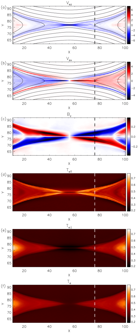
Figure 2: Basic reconnection parameters for run 46. (a) $V_{ez}$ and (b) $V_{ex}$ with magnetic field lines, (c) $B_{z}$, (d) $T_{e||}$, (e) $T_{e\perp}$, and (f) $T_{e}=(T_{e||}+2\,T_{e\perp})/3$. Note that plots (d), (e), and (f) are on the same color scale for easy comparison. The vertical dashed lines show the location of the cut for Figure 3.

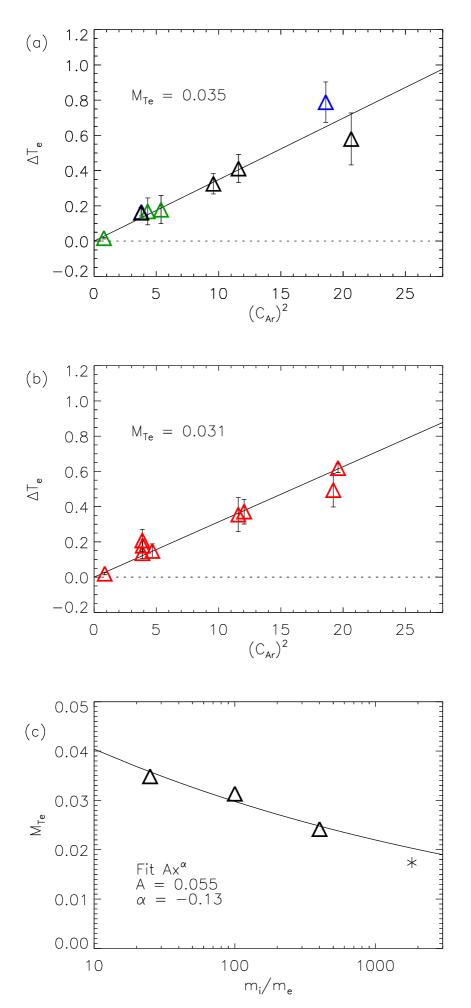
Figure 7: Effect of Mass ratio on Electron Heating. (a) $m_{i}/m_{e}=25$ and (b) $m_{i}/m_{e}=100$ simulations with the same parameters except for mass ratio. (c) $M_{Te}$ versus mass ratio. Note that the $m_{i}/m_{e}=400$ point is from a single simulation. The coloring of points in panels (a) and (b) uses the same convention as in Figure 4. The simulations used for this figure are shown in Table 1 with a check mark in the “$m_{i}/m_{e}$ compare” column.