A 1-parameter family of spherical CR uniformizations of the figure eight knot complement

Abstract.

We describe a simple fundamental domain for the holonomy group of the boundary unipotent spherical CR uniformization of the figure eight knot complement, and deduce that small deformations of that holonomy group (such that the boundary holonomy remains parabolic) also give a uniformization of the figure eight knot complement. Finally, we construct an explicit 1-parameter family of deformations of the boundary unipotent holonomy group such that the boundary holonomy is twist-parabolic. For small values of the twist of these parabolic elements, this produces a 1-parameter family of pairwise non-conjugate spherical CR uniformizations of the figure eight knot complement.

1. Introduction

The existence of a complete hyperbolic structure on a 3-manifold has important topological consequences. For instance, this gives a definition of the volume of a knot (when a knot admits a complete hyperbolic structure, that structure is unique by Mostow rigidity, so the volume of that metric is a well-defined invariant).

In this paper, we focus on another kind of geometric structures on 3-manifolds, namely structures modeled on the boundary of a symmetric space $X$ of negative curvature (transition maps are required to be locally given by isometries of $X$). The visual boundary $\partial_{\infty}X$ is then a 3-dimensional sphere if $X=H^{4}_{\mathbb{R}}$ or $H^{2}_{\mathbb{C}}$.

The first case gives rise to the theory of flat conformal structures, and the second one to the theory spherical CR structures. In the first case, one considers the unit ball model of $H^{4}_{\mathbb{R}}$, so the visual boundary is $S^{3}\subset\mathbb{R}^{4}$, and the group of isometries of $H^{4}_{\mathbb{R}}$ acts as Möbius transformations (i.e. transformations that map spheres into spheres, of possibly infinite radius). Alternatively, one can use stereographic projection and think of $S^{3}$ as $\mathbb{R}^{3}\cup\{\infty\}$; this would also correspond to using the upper half plane model for $H^{3}_{\mathbb{R}}$.

In the second case, using the ball model $\mathbb{B}^{2}\subset\mathbb{C}^{2}$ one can identify $\partial_{\infty}H^{2}_{\mathbb{C}}$ with the unit sphere $S^{3}\subset\mathbb{C}^{2}$. The action on the boundary is best understood in stereographic projection, and identifying $S^{3}\setminus\{p_{\infty}\}\simeq\mathbb{R}^{3}\simeq\mathbb{C}\times\mathbb{R}$ with the Heisenberg group. Isometries of $H^{2}_{C}$ fixing $p_{\infty}$ then acts as automorphisms of the Heisenberg group. Of course the Heisenberg group acting on itself by left translations gives many automorphisms (which correspond to the action of unipotent matrices in $U(2,1)$), and one gets the full automorphism group by adjoining a rotation in $\mathbb{C}\times\mathbb{R}$ around the $\mathbb{R}$ factor, and scaling of the form $(z,t)\mapsto(\lambda z,\lambda^{2}t)$ (which corresponds to a loxodromic isometry), see section 3.2.

Even though a lot of partial results have been obtained (see [18], [13] for instance), the classification of 3-manifolds that admit a spherical CR structure is far from understood. When a manifold admits a spherical CR structure, the moduli space of such structures is also quite mysterious.

In this paper, we will be interested in a special kind of spherical CR structures, namely spherical CR uniformizations (in the literature, these are sometimes called complete spherical CR structures). These are characterized by the fact that the developing map of the structure is a diffeomorphism onto its image, which is an open set in $S^{3}$. In that case, the holonomy group is a discrete subgroup $\Gamma\subset PU(2,1)$, and the image of the developing map is the domain of discontinuity $\Omega_{\Gamma}$ of $\Gamma$ (i.e. the largest open set where the action is proper). The quotient $\Gamma\setminus\Omega_{\Gamma}$ is called the manifold at infinity of $\Gamma$.

The classification of 3-manifolds that admit a spherical CR uniformization is also an open problem. Recall that $H^{2}_{\mathbb{C}}$ is a homogeneous under the action of $PU(2,1)$, and the isotropy group of a point is isomorphic to $U(2)$. In particular, finite subgroups of $U(2)$ such that nontrivial elements fix only the origin (in other words the groups should not contain any complex reflection) yield spherical CR uniformizable 3-manifolds with finite fundamental group.

In a similar vein, quotients of the Heisenberg group yield Nil manifolds that trivially admit a spherical CR uniformization, such that the holonomy group has a global fixed point, which is now in $\partial_{\infty}H^{2}_{\mathbb{C}}$ instead of $H^{2}_{\mathbb{C}}$.

It is also natural to consider stabilizers of totally geodesic subspaces in $H^{2}_{\mathbb{C}}$, namely copies of $H^{2}_{\mathbb{R}}$ or $H^{1}_{\mathbb{C}}$. In that setting, Fuchsian groups (i.e. discrete subgroups of $SO(2,1)$ or $SU(1,1)$, seen as subgroups of $SU(2,1)$) produce as their manifold at infinity a circle bundle over a surface (or more generally over a 2-orbifold). This class is more interesting than the previous one, because it is known that the corresponding groups often admit deformations (but not always, see [29]). We will summarize the results in this well developed line of research by saying simply that many Seifert 3-manifolds admit spherical CR uniformizations (see [15], [1], [20], [30] and others).

The class of hyperbolic manifolds that admit a spherical CR uniformization is also far from being understood. In a number of beautiful results that appeared in the last decade, Schwartz discovered that many hyperbolic manifolds admit spherical CR uniformizations, see [25], [27] and [28]. His starting point was to consider representations of triangle groups into $PU(2,1)$, see [26], and to determine the manifold at infinity of well chosen such representations.

More recently, the figure eight knot complement was shown to admit a spherical CR uniformization [7] by following a somewhat different strategy, namely it was found as a byproduct of Falbel’s program for finding representations of fundamental groups of triangulated 3-manifold into $PU(2,1)$ (see [9]), or in $PGL(3,\mathbb{C})$ (see [3]).

Falbel’s construction turned out to produce lots of representations, and in fact so many that the geometric properties of the resulting representations are in general difficult to analyze. In order to make the list more tractable (and also for other reasons related to the study of Bloch groups), the search is often restricted to representations such that peripheral subgroups are mapped to unipotent matrices (matrices with 1 as their only eigenvalue). The boundary unipotent representations for non-compact 3-manifolds with low complexity (i.e those that can be built by gluing up to three ideal tetrahedra) are listed in [11], and the geometry of some of these representations are analyzed in [7] and [6]. It turns out very few representations in that list are discrete.

It is quite clear however that the unipotent restriction is somewhat artificial. Part of the point of the present paper is to show that, at least in some cases, there are many boundary parabolic representations that are not unipotent, and that these representations carry just as much interesting geometric information about the 3-manifold.

Let $M$ denote the figure eight knot complement. The main goal of this paper is to show that $M$ admits a 1-parameter family of pairwise non conjugate spherical CR uniformizations.

We will build on the fact that $M$ admits a unique spherical CR uniformization with unipotent boundary holonomy, as was shown in [7]. For future reference, we will refer to that structure simply as the boundary unipotent uniformization of $M$ (see the precise uniqueness statement in [7]), and we denote the corresponding holonomy representation by $\rho$. In view of Schwartz’s spherical CR Dehn surgery theorem [28], one expects that small deformations of the boundary unipotent holonomy representation should still be discrete, and they should have a manifold at infinity given by some Dehn filling of the figure eight knot complement.

In order to turn this into a proof, one could try and prove that the boundary unipotent representation satisfies the hypotheses of Schwartz’s theorem, i.e. that its image is a horotube group (without exceptional parabolic elements), and that its limit set is porous. If that works, then it is enough to show that the group admits deformations, and to study the type of the deformed unipotent element; Schwartz’s surgery formula shows in particular that (under some technical assumptions), if there are deformations where the unipotent peripheral holonomy stays parabolic, then the manifold at infinity should not change at all in small deformations.

Although a few examples of non-compact hyperbolic manifolds are known to admit spherical CR uniformizations (see [25], [27], [7]), the deformation theory of the holonomy representations of these examples is still quite mysterious. In particular, there are only two examples where non-trivial deformations are known to exist such that peripheral elements map to parabolic elements. These two examples are the figure eight knot complement and the Whitehead link complement. The results announced by Parker and Will, see [21] say that there are at least two different spherical CR uniformizations of the Whitehead link complement, and that there is a 1-parameter family of representations interpolating between their holonomy representations.

The main result of our paper gives an explicit construction of twist-parabolic deformations.

Theorem 1.1.

There is a continuous 1-parameter family of irreducible representations $\rho_{t}:\pi_{1}(M)\rightarrow PU(2,1)$, such that for each $t$, $\rho_{t}$ maps peripheral subgroups of $M$ onto a cyclic group generated by a single parabolic element with eigenvalues $e^{it},e^{it},e^{-2it}$.

Given the eigenvalue condition, it should be clear that the representations $\rho_{t}$ are pairwise non conjugate. We will choose $\rho_{t}$ so that $\rho_{0}$ is the holonomy of the boundary unipotent spherical CR uniformization.

Note that the existence of such parabolic deformations was independtly discovered by Pierre-Vincent Koseleff, using a variant of the method devised by Falbel to parametrize boundary unipotent representations of 3-manifolds, see [9], [3] and [11] for instance. An alternative parametrization of this family can also be obtained from the description of the full character variety, see [10], see also [17].

We will use a more naïve construction, which is closer in spirit to Riley’s parametrization of the character variety of the figure eight knot group (or more generally 2-bridge knot groups) into $PSL_{2}(\mathbb{C})$, see [23].

Our main result is the following.

Theorem 1.2.

There exists a $\delta>0$ such that for $|t|<\delta$, $\rho_{t}$ is the holonomy of a spherical CR uniformization of the figure eight knot complement.

In order to show this, we will study the Ford domain for the image of $\rho_{0}$, and we will show that it is generic enough for its combinatorics to be preserved under small deformations of $\rho_{0}$. Note that this argument turns out to fail for the Ford domain of the holonomy of the spherical CR uniformization of the Whitehead link complement announced by Parker and Will in [21]. Indeed, their Ford domain has the same local combinatorial structure as the Dirichlet domain described in [7], and in particular it has lots of tangent spinal spheres.

It will be clear to the reader familiar with the notion of horotubes [28] that the Ford domain exhibits an explicit horotube structure for the group, but since our construction of horotubes is actually very close to proving Theorem 1.2, we will give a detailed argument that does not quote Schwartz’s result. Of course in many places, our proof parallels some of the intermediate results in  [28].

We will not attempt to give an explicit allowable range of parameters $t$ in Theorem 1.2, although it would certainly be interesting to do so (and also to try and make this range optimal).

The bulk of the work will be to describe the Ford domain for the holonomy group of the unipotent uniformization of $M$, and to study in detail the generic character of the intersection of its sides, along facets of all dimensions. The genericity that we will prove is genericity at infinity, namely we will show that each ideal vertex in the Ford domain lies on precisely three sides that intersect transversely at that point. For finite vertices, no genericity is to be expected, since the group is known to contain elliptic elements of order 3 and 4 (see [7]). In fact all the deformations we consider will preserve the conjugacy classes of these elliptic elements, and we will show that they do not affect the non-generic character of the fundamental domains at these points:

Proposition 1.3.

The image of $\rho_{t}$ is a triangle group. More specifically, for all $t$, we have

$$\rho_{t}(g_{2})^{4}=\rho_{t}(g_{1}g_{2})^{3}=\rho_{t}(g_{2}g_{1}g_{2})^{3}=id.$$

Acknowledgements: This work was partly supported by the ANR, through the grant SGT (“Structures Géométriques Triangulées”). I also benefited from generous support from the GEAR network (NSF grants DMS 1107452, 1107263, 1107367), via funding of a long term visit at ICERM. I am pleased to thank ICERM for its hospitality, and the participants of the semester program entitled “Low-dimensional Topology, Geometry, and Dynamics” for inspiring interactions. Finally, I would like to thank the referee for several suggestions that helped improve the readability of the paper.

2. The real hyperbolic Ford domain

Throughout this section, we denote by $M$ the figure eight knot complement. We review the description of a cusp neighborhood for $M$. This is probably familiar to most readers, but the details will be used in the identification of the manifold at infinity of our complex hyperbolic groups. Moreover, quite remarkably, the local combinatorics of the real hyperbolic Ford domain turn out to be exactly the same as the local combinatorics of our fundamental domain for the action of the group on the domain of discontinuity.

Recall that the fundamental group $\pi_{1}(M)$ has a presentation of the form

$$\langle\,g_{1},g_{2},g_{3}\,|\,g_{2}=[g_{3},g_{1}^{-1}],g_{1}g_{2}=g_{2}g_{3}\,\rangle,$$

with peripheral subgroup generated by $g_{3}^{-1}$ and $g_{1}(g_{1}g_{2})^{-1}g_{3}g_{2}g_{3}^{-1}$.

From this, one can find all type-preserving representations of $\pi_{1}(M)$ up to conjugation, as in [22]. Indeed, the generators $g_{1}$ and $g_{3}$ should be parabolic elements in $SL_{2}(\mathbb{C})$, which we denote by $G_{1}$ and $G_{3}$. We may assume $G_{1}$ (resp. $G_{3}$) fixes $0$ (resp. $\infty$), and since all parabolic elements are conjugate, we may also assume

$$G_{1}=\begin{pmatrix}1&0\\ -\omega&1\end{pmatrix};G_{3}=\begin{pmatrix}1&1\\ 0&1\end{pmatrix}$$

for some $\omega\in\mathbb{C}$. The relation $G_{1}[G_{3},G_{1}^{-1}]=[G_{3},G_{1}^{-1}]G_{3}$ in $PSL_{2}(\mathbb{C})$, is easily seen to imply $\omega^{2}+\omega+1$, so we may take

$$\omega=\frac{-1+i\sqrt{3}}{2}.$$

The stabilizer of $\infty$ in $PSL_{2}(\mathbb{Z}[\omega])$ is clearly given by translations by Eisenstein integers, but the stabilizer in the group generated by $G_{1}$ and $G_{3}$ is slightly smaller, it can be checked to be generated by translations by $1$ and $2i\sqrt{3}$ (see [22] for more details).

Recall that the Ford isometric sphere of an element

$$\begin{pmatrix}a&b\\ c&d\end{pmatrix}$$

is bounded by the circle $|cz+d|=1$. The Ford domain turns out to be the intersection of the exteriors of all spheres of radius 1 centered at Eisenstein integers. A schematic picture is shown in Figure 1, where the sides corresponding to $G_{1}^{\pm 1}$ (resp. $G_{2}^{\pm 1}=[G_{3},G_{1}^{-1}]^{\pm 1}$) are shaded in the same color, so the corresponding $2$-faces get identified by the corresponding isometries.

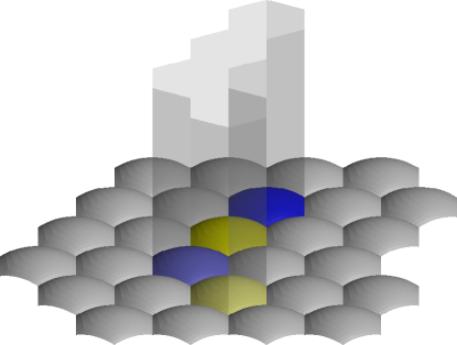
Figure 1. A fundamental domain for the action of $\Gamma$ is an infinite chimney over the union of four hexagons, each hexagons living in a unit hemisphere around the appropriate Eisenstein integer.

The complete description of identifications on bottom face of the prism is given in Figure 2, and there are also identifications on the vertical sides of the prism, which are simply given by translations whenever these sides are parallel.

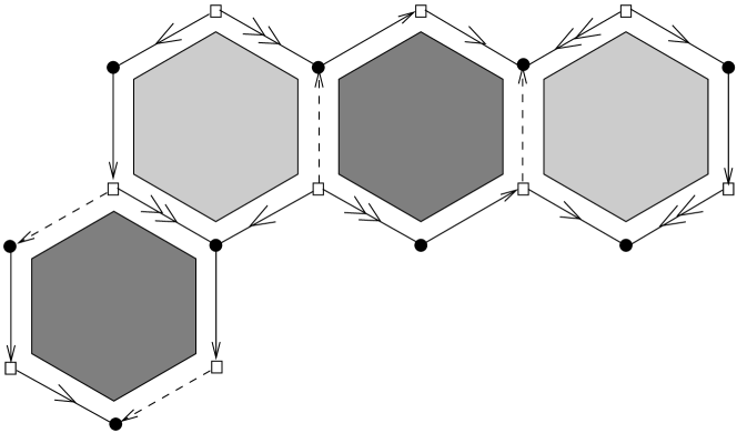
Figure 2. Bottom of the prism (spine of the figure eight knot complement).

Note that these identifications are described in [22]; using current computer technology, they can also be found using the pictures produced by SnapPy.

3. Basic complex hyperbolic geometry

In this section we review some basic material about the complex hyperbolic plane. The reader can find more details in [14].

Recall that $\mathbb{C}^{2,1}$ denotes $\mathbb{C}^{3}$, equipped with a Hermitian form of signature (2,1). The standard such form is given by $\langle V,W\rangle=V_{1}\overline{W}_{3}+V_{2}\overline{W}_{2}+V_{3}\overline{W}_{1}=W^{*}JV$, where

$$J=\left(\begin{matrix}0&0&1\\ 0&1&0\\ 1&0&0\end{matrix}\right).$$

We denote by $U(2,1)$ the subgroup of $GL(3,\mathbb{C})$ that preserves that Hermitian form, and by $PU(2,1)$ the same group modulo scalar matrices. It is sometimes convenient to work with $SU(2,1)$, which is a 3-fold cover of $PU(2,1)$.

The complex hyperbolic plane $H^{2}_{\mathbb{C}}$ is the set of negative complex lines in $\mathbb{C}^{2,1}$, equipped with a Kähler metric that is invariant under the action of $PU(2,1)$. Such a metric is unique up to scaling, and it turns out to have constant holomorphic sectional curvature (which one can choose to be -1).

It is well known that the maximal totally geodesic submanifolds of $H^{2}_{\mathbb{C}}$ are copies of $H^{1}_{\mathbb{C}}$ (with curvature -1) and copies of $H^{2}_{\mathbb{R}}$ (with curvature $-1/4$).

3.1. Bisectors

The corresponding distance function is given by

$$\cosh^{2}\frac{1}{2}d(z,w)=\frac{|\langle Z,W\rangle|^{2}}{\langle Z,Z\rangle\langle W,W\rangle},$$

where $Z$ (resp. $W$) denotes a representative of $z$ (resp. $w$). Given two points $p\neq q\in H^{2}_{\mathbb{C}}$, the locus $\mathcal{B}(p,q)$ of points that are equidistant of $p$ and $q$ is called a bisector. Beware that isometries switching $p$ and $q$ do not fix the corresponding bisector pointwise, and in fact bisectors are not totally geodesic. The copies of ${{\bf H}^{1}_{\mathbb{C}}}$ (resp. ${{\bf H}^{2}_{\mathbb{R}}}$) in $\mathcal{B}(p,q)$ are called its complex (resp. real) slices. All real slices intersect along the same real geodesic, called the real spine of the bisector (see [14]).

Every bisector in $H^{2}_{\mathbb{C}}$ is diffeomorphic the unit ball in $\mathbb{R}^{3}$, in such a way that the vertical axis is the real spine, complex slices are horizontal disks, and real slices are disks in vertical planes containing the vertical axis. One way to do this explicitly for the bisector $\mathcal{B}(p,q)$ is to scale $q$ by a complex number of modulus one so that $\langle p,q\rangle$ is real and negative. Then an orthogonal basis for $\mathbb{C}^{2,1}$ is given by $v_{0}=p+q$, $v_{1}=p-q$, $v_{2}=v_{0}\boxtimes v_{1}$ ($\boxtimes$ denotes the Hermitian cross product, see p.43 of [14]). Of course this basis can be made Lorentz orthonormal by scaling its vectors so that $\langle v_{0},v_{0}\rangle=-1$, $\langle v_{1},v_{1}\rangle=1$ and $\langle v_{2},v_{2}\rangle=1$. The bisector then can be parametrized by $(z,t)\in\mathbb{C}\times\mathbb{R}$ by taking vectors of the form

$$v_{0}+i\,t\,v_{1}+z\,v_{2}.$$

Given a set $S\subset H^{2}_{\mathbb{C}}$, we write $\mathcal{B}(S)$ for the locus equidistant of all point in $S$, which can be thought of as an intersection of bisectors.

The intersection of two bisectors is usually not totally geodesic, but it can be in some rare instances. When $p$, $q$ and $r$ are not in a common complex line (i.e. when lifts of these vectors are linearly independent), the locus $\mathcal{B}(p,q,r)$ of points equidistant of $p$, $q$ and $r$ is a smooth non totally geodesic disk, and is often called a Giraud disk, see [12]. The following property is crucial when studying fundamental domains (see [12], [14]).

Theorem 3.1.

If $p$, $q$ and $r$ are not in a common complex line, then $\mathcal{B}(p,q,r)$ is contained in precisely three bisectors, namely $\mathcal{B}(p,q)$, $\mathcal{B}(q,r)$ and $\mathcal{B}(q,r)$.

Note that checking whether an isometry maps a Giraud disk to another is equivalent to checking that the corresponding triple of points are mapped to each other.

In order to study Giraud disks, we will use spinal coordinates. The complex slices of $\mathcal{B}(p,q)$ are given explicitly by choosing a lift $\tilde{p}$ (resp. $\tilde{q}$) of $p$ (resp. $q$).

When $p,q\in H^{2}_{\mathbb{C}}$, we simply choose lifts such that $\langle\tilde{p},\tilde{p}\rangle=\langle\tilde{q},\tilde{q}\rangle$. In this paper, we will mainly use these parametrization when $p,q\in\partial_{\infty}H^{2}_{\mathbb{C}}$. In that case, the condition $\langle\tilde{p},\tilde{p}\rangle=\langle\tilde{q},\tilde{q}\rangle$ is vacuous, since all lifts are null vectors; we then choose some fixed lift $\tilde{p}$ for the center of the Ford domain, and we take $\tilde{q}=G\tilde{p}$ for some $G\in U(2,1)$. If a different matrix $G^{\prime}=SG$, with $S$ a scalar matrix, note that the diagonal element of $S$ is a unit complex number, so $\tilde{q}$ is well defined up to a unit complex number.

The complex slices of $\mathcal{B}(p,q)$ are obtained as (the set of negative lines in) $(\bar{z}\tilde{p}-\tilde{q})^{\perp}$ for some arc of values of $z\in S^{1}$, which is determined by requiring that $\langle\bar{z}\tilde{p}-\tilde{q},\bar{z}\tilde{p}-\tilde{q}\rangle>0$.

Since a point of the bisector is on precisely one complex slice, we can parametrize $\mathcal{B}(p,q,r)$ by $(z_{1},z_{2})\in S^{1}\times S^{1}$ via

(1) $$V(z_{1},z_{2})=(\bar{z}_{1}p-q)\boxtimes(\bar{z}_{2}p-r)=q\boxtimes r+z_{1}\ r\boxtimes p+z_{2}\ p\boxtimes q.$$

The Giraud disk corresponds to the $(z_{1},z_{2})\in S^{1}\times S^{1}$ such that $\langle V(z_{1},z_{2}),V(z_{1},z_{2})\rangle<0$ (it follows from the fact that the bisectors are covertical that this region is a topological disk, but this is not obvious, see chapters 8 and 9 in [14]).

The boundary at infinity $\partial_{\infty}\mathcal{B}(p,q,r)$ is a circle, given in spinal coordinates by the equation

(2) $$\langle V(z_{1},z_{2}),V(z_{1},z_{2})\rangle=0$$

Note that the choice of two lifts of $q$ and $r$ affects the spinal coordinates by rotation on each of the $S^{1}$ factors.

A defining equation for the trace of another bisector $\mathcal{B}(a,b)$ on the Giraud disk $\mathcal{B}(p,q,r)$ can be written in the form

(3) $$|\langle V(z_{1},z_{2}),a\rangle|=|\langle V(z_{1},z_{2}),b\rangle|,$$

provided $a,b$ are suitably chosen lifts. The expressions $\langle V(z_{1},z_{2}),a\rangle$ and $\langle V(z_{1},z_{2}),b\rangle$ are affine in $z_{1}$, $z_{2}$.

These triple bisector intersections can be parametrized fairly explicitly, because one can solve the equation $|\langle V(z_{1},z_{2}),a\rangle|^{2}=|\langle V(z_{1},z_{2}),b\rangle|^{2}$ for one of the variables $z_{1}$ or $z_{2}$, simply by solving a quadratic equation. A detailed explanation of how this works can be found in section 2.3 of [7], we will also review this in section 5.3.3.

Note that our parameters also give a parametrization of the intersection in $P^{2}_{\mathbb{C}}$ of the extors extending the bisectors, see chapter 8 of [14]. The Giraud disk is a disk in the intersection of the extors, which is a torus.

3.2. Siegel domain and the Heisenberg group

The complex analogue of the upper half space model for $H^{n}_{\mathbb{R}}$ is the Siegel domain, which is obtained by sending the line spanned by $(1,0,0)$ to infinity. We denote the corresponding point of $\partial_{\infty}H^{2}_{\mathbb{C}}$ by $p_{\infty}$.

More precisely, we take affine coordinates $z_{1}=Z_{1}/Z_{3}$, $z_{2}=Z_{2}/Z_{3}$, and a negative complex line has a unique representative of the form $z=(z_{1},z_{2},1)$ with

$$z^{*}Jz=2\mathfrak{Re}(z_{1})+|z_{2}|^{2}<0$$

Since we are interested in geometric structures modeled on $\partial_{\infty}H^{2}_{\mathbb{C}}$, we will use mainly the boundary of the Siegel domain, which is given by points $z=(z_{1},z_{2},1)$ with $2\mathfrak{Re}(z_{1})+|z_{2}|^{2}=0$. It is best understood in terms of Heisenberg geometry, as we now briefly recall.

A large part of the stabilizer of the point at infinity is given by unipotent upper triangular matrices. One easily checks that such a matrix preserve the Hermitian form $J$ if and only if it can be written as

$$\left(\begin{matrix}1&-\bar{a}\sqrt{2}&-|a|^{2}+is\\ 0&1&a\sqrt{2}\\ 0&0&1\end{matrix}\right)$$

for some $(a,s)\in\mathbb{C}\times\mathbb{R}$. Since these upper triangular matrices form a group, we get a group law on $\mathbb{C}\times\mathbb{R}$, given by

(4) $$(a,s)*(a^{\prime},s^{\prime})=(a+a^{\prime},s+s^{\prime}+2\Im(a\,\bar{a}^{\prime})).$$

This is the so-called Heisenberg group law.

The action of the unipotent stabilizer of $p_{\infty}$ is simply transitive on $\partial_{\infty}H^{2}_{\mathbb{C}}-\{p_{\infty}\}$, so we will often identify the latter with $\mathbb{C}\times\mathbb{R}$.

The boundary at infinity of totally geodesic subspaces can be seen in somewhat simple terms in $\mathbb{C}\times\mathbb{R}$. The boundary of a copy of $H^{1}_{\mathbb{C}}$ (which is the intersection of an affine line in $\mathbb{C}^{2}$ with the Siegel half space) is called a $\mathbb{C}$-circle. These are ellipses that project to circles in $\mathbb{C}$ (or possibly vertical lines, if they go through $p_{\infty}$).

The boundary of copies of $H^{2}_{\mathbb{R}}$ (which are images under arbitrary isometries of the set of real points in the Siegel half space) intersect the boundary at infinity in a so-called $\mathbb{R}$-circle. In the Heisenberg group, these are curves that project to lemniscates in $\mathbb{C}$ (or possibly straight lines when they go through $p_{\infty}$). For more on this, see chapter 4 of [14], for instance.

The full stabilizer of $p_{\infty}$ is generated by the above unipotent group, together with the isometries of the form

$$\left(\begin{matrix}1&0&0\\ 0&e^{i\theta}&0\\ 0&0&1\end{matrix}\right),\quad\left(\begin{matrix}\lambda&0&0\\ 0&1&0\\ 0&0&1/\lambda\end{matrix}\right),$$

where $\theta,\lambda\in\mathbb{R}$, $\lambda\neq 0$. The first one acts on Heisenberg as a rotation with vertical axis:

$$(a,s)\mapsto(e^{i\theta}a,s),$$

whereas the second one acts as

$$(a,s)\mapsto(la,l^{2}s).$$

There is a natural invariant metric on the Heisenberg group, called the Cygan metric, given by $d(g,g^{\prime})=||g^{-1}g^{\prime}||$, and the norm of an element of the Heisenberg group is given by

(5) $$||(z,t)||=||z|^{2}+it|^{1/2}$$

The Cygan sphere with center $(z_{0},t_{0})$ and radius $r$ has equation

(6) $$\left||z-z_{0}|^{2}+i(t-t_{0}+2\Im(z\bar{z}_{0}))\right|=r^{2}.$$

3.3. Ford domains and the Poincaré polyhedron theorem

Let $\Gamma$ be a subgroup of $PU(2,1)$, let $q\in\partial_{\infty}H^{2}_{\mathbb{C}}$ and let $Q$ denote a lift of $q$ in $\mathbb{C}^{2,1}$.

Definition 3.2.

The Ford domain for $\Gamma$ centered at $q$ is the set $F_{\Gamma,q}$ of points $z\in H^{2}_{\mathbb{C}}$ such that

$$|\langle Z,Q\rangle|\leq|\langle Z,G(Q)\rangle|$$

where $G$ is a matrix representative of some element $g\in\Gamma$.

The inequality is actually independent of the lift $G\in U(2,1)$ chosen for $g\in PU(2,1)$. For a given $g\in\Gamma$ and lift $G\in U(2,1)$, we denote by $\mathcal{B}_{g}$ the bisector given in homogeneous coordinates by

(7) $$|\langle Z,Q\rangle|=|\langle Z,G(Q)\rangle|.$$

For concreteness, we mention that the boundary at infinity of $\mathcal{B}_{g}$ can be described as a Cygan sphere in the Heisenberg group (see section 3.2). The Cygan sphere corresponding to an element $G$ has radius $\sqrt{2/|g_{31}|}$ (note that $G$ fixes $p_{\infty}$ if and only if $g_{31}=0$) and center $(\bar{g}_{32}/\bar{g}_{31},2\Im(\bar{g}_{33}/\bar{g}_{31})$ (see equation (6)).

We denote by $b_{g}=\mathcal{B}_{g}\cap F$, i.e. the side of $F$ that lies on the bisector $\mathcal{B}_{g}$, and we refer to it as the side corresponding to the group element $g$. For a general $g\in\Gamma$, $b_{g}$ may have dimension smaller than 3 (in fact it is often empty). The bisectors of the form $\mathcal{B}_{g}$ such that $b_{g}$ have dimension three will be called bounding bisectors.

The basic fact is that if $q$ has trivial stabilizer in $\Gamma$, then $F=F_{\Gamma,q}$ is a fundamental domain for its action. However, it is customary to take $q$ to have a nontrivial stabilizer $H\subset\Gamma$, in which case $F$ is only a fundamental domain modulo the action of $H$. In other words, in that case, $F$ is a fundamental domain for the decomposition of $\Gamma$ into cosets of $H$.

It is ususally very hard to determine $F$ explicitly; in order to prove that a given polyhedron is equal to $F$, the main tool is the Poincaré polyhedron theorem. The basic idea is that the sides of $F$ should be paired by isometries, and the images of $F$ under these so-called side-pairing maps should give a local tiling of $H^{2}_{\mathbb{C}}$. If they do (and if the quotient of $F$ by the identifications given by the side-pairing maps is complete), then the Poincaré polyhedron implies that the images of $F$ actually give a global tiling.

Once a fundamental domain is obtained, one gets an explicit presentation of $\Gamma$ in terms of the generators given by the side-pairing maps together with a generating set for the stabilizer $H$, the relations corresponding to so-called ridge cycles (which correspond to the local tiling near each codimension two face).

For more details on this theorem, see [7], [8] and [19].

4. A boundary parabolic family of representations

In this section, we parametrize a neighborhood of the unipotent solution in the character variety $\chi(\pi_{1}(M),PU(2,1))$. We will use the presentation

$$\langle\ g_{1},g_{2},g_{3}\ |\ g_{1}g_{2}=g_{2}g_{3},g_{2}=[g_{3},g_{1}^{-1}]\ \rangle.$$

In order to describe representations, we seek to parametrize triples $G_{1},G_{2},G_{3}$ of matrices in $SU(2,1)$ that satisfy the same relations as $g_{1}$, $g_{2}$, $g_{3}$ (possibly up to multiplication by a scalar matrix, since we are really after representations in $PU(2,1)$).

If the fixed points of $G_{1}$ and $G_{3}$ are distinct, we may assume

(8) $$G_{1}=\left(\begin{matrix}\lambda&a&b\\ 0&\overline{\lambda}^{2}&c\\ 0&0&\lambda\end{matrix}\right),\quad G_{3}=\left(\begin{matrix}\lambda&0&0\\ f&\overline{\lambda}^{2}&0\\ e&d&\lambda\end{matrix}\right),$$

were $|\lambda|=1$.

Note that the representation considered in [7] is obtained by taking

$$\lambda=1,a=d=1,c=f=-1,b=\overline{e}=-(1+i\sqrt{7})/2$$

in equation (8).

The fact that $G_{1}$ and $G_{3}$ are isometries of the form $J$ implies

(9) $$\left\{\begin{array}[]{l}c=-\overline{a}\,\overline{\lambda},\quad f=-\overline{d}\,\overline{\lambda}\\ |d|^{2}+\overline{e}\lambda+e\overline{\lambda}=0\\ |a|^{2}+\overline{b}\lambda+b\overline{\lambda}=0\end{array}\right.$$

We then compute the commutator $G_{2}=[G_{3},G_{1}^{-1}]$, and consider the system of equations given by $R=0$, where

(10) $$R=G_{1}G_{2}-G_{2}G_{3}.$$

Note that this already restricts the character variety, since we only consider representations into $U(2,1)$ rather than $PU(2,1)$, but this is fine if we are after a neighborhood of the boundary unipotent solution, where the relation (10) holds in $U(2,1)$.

Requiring that $G_{1}$ and $G_{3}$ preserve the standard antidiagonal form, we must have

The $(1,1)$-entry of $R$ is given by

(11) $$(|a|^{2}e-|d|^{2}b)(1+\overline{a}d-\lambda^{3}-\overline{\lambda}^{3}).$$

The first factor does not vanish for the boundary unipotent solution, so in its component we must have

(12) $$1+\overline{a}d=\lambda^{3}+\overline{\lambda}^{3}.$$

Note that by conjugation by a diagonal matrix with diagonal entries $k_{1},k_{2},k_{3}$, we can assume that $a\in\mathbb{R}$ (and we can also impose that $|b|$ is given by any positive real number). Equation (12) then implies that $d$ is real as well, so from this point on we assume

$$a,d\in\mathbb{R}.$$

The $(2,2)$-entry of $R$ can then be written as

$$-(|a|^{2}e-|d|^{2}b)(a^{2}e\overline{\lambda}^{4}+a^{2}d^{2}\overline{\lambda}^{3}-ad+be\overline{\lambda}^{5}-1+bd^{2}\overline{\lambda}^{4}),$$

so we get the equation

(13) $$a^{2}e\overline{\lambda}^{4}+a^{2}d^{2}\overline{\lambda}^{3}-ad+be\overline{\lambda}^{5}-1+bd^{2}\overline{\lambda}^{4}.$$

Using the relations (9) and (12), (13), can be rewritten as

(14) $$be\lambda=\lambda^{3}+\overline{\lambda}^{3}.$$

As mentioned above, by conjugation by a diagonal matrix, we can adjust $|b|$, for instance so that

$$|b|^{2}=\lambda^{3}+\overline{\lambda}^{3},$$

and in that case (14) implies

$$|e|^{2}=|b|^{2}.$$

We will now show that, given $\lambda$, the following system has precisely two solutions:

(15) $$\left\{\begin{array}[]{l}a^{2}+\overline{b}\lambda+b\overline{\lambda}=0\\ d^{2}+\overline{e}\lambda+e\overline{\lambda}=0\\ 1+ad=\lambda^{3}+\overline{\lambda}^{3}\\ eb\lambda=\lambda^{3}+\overline{\lambda}^{3}\\ |b|^{2}=\lambda^{3}+\overline{\lambda}^{3}.\end{array}\right.$$

In order to do that, note that the first four imply

$$b\overline{e}+\overline{b}e=1-2(\lambda^{3}+\overline{\lambda}^{3}),$$

and the last two imply

$$e=\overline{b}\overline{\lambda}.$$

Putting these two together, we get

(16) $$\Re(b^{2}\lambda)=\frac{1}{2}-2\kappa,$$

where we have written

(17) $$\kappa=(\lambda^{3}+\overline{\lambda}^{3})/2.$$

The equation $\Re(z)=\frac{1}{2}-2\kappa$ has a solution with $|z|=2\kappa$ if and only if

$$2\kappa\geq\frac{1}{2}-2\kappa,$$

and in that case one gets a simple formula for the solutions (intersect a vertical line with the circle of radius $|2\kappa|$ centered at the origin).

We get that (16) has solutions if and only if $\kappa\geq\frac{1}{8}$, and the solutions are given by

(18) $$b^{2}\lambda=\frac{1}{2}-2\kappa\pm i\sqrt{\frac{1}{2}(4\kappa-\frac{1}{2})}.$$

This determines $b$ up to its sign, opposite values clearly giving conjugate groups (they differ by conjugation by a diagonal matrix). The two values also yield isomorphic groups, obtained from each other by complex conjugation.

We will choose the solution to match the notation for the unipotent solution given in [7], which corresponds to $\lambda=1$, $a=d=1$, $b=-\frac{1+i\sqrt{7}}{2}$ and $e=-\frac{1-i\sqrt{7}}{2}$.

As a consequence, we take

$$b=-\frac{1+i\sqrt{8\kappa-1}}{2\sqrt{\lambda}},$$

where we take the squareroot to vary continuously near $\lambda=1$.

The system (15) then gives values for the other parameters, namely

$$e=2\kappa/b\lambda=-\frac{1-i\sqrt{8\kappa-1}}{2\sqrt{\lambda}},$$

and one easily writes an explicit formula for $a$ and $d$ (once again, these are determined only up to sign, but changing $a$ to $-a$ can be effected by conjugation by a diagonal matrix). The formula is as follows,

$$a=\sqrt{(4\mu^{2}-3)\mu+\sqrt{8\kappa-1}(4\mu^{2}-1)\nu},\quad d=\sqrt{(4\mu^{2}-3)\mu-\sqrt{8\kappa-1}(4\mu^{2}-1)\nu},$$

where we have written $\sqrt{\lambda}=\mu+i\nu$ with $\mu$, $\nu$ real. In terms of this new parameter, the condition $\kappa>1/8$ translates into

$$\mu>\cos(\frac{1}{3}\arctan\frac{\sqrt{7}}{3})=0.9711209254\dots$$

In fact, in order to get $a$ and $d$ to be real, we also need

$$(4\mu^{2}-3)\mu-\sqrt{8\kappa-1}(4\mu^{2}-1)\nu\geq 0,$$

which translates into $\mu\geq\cos(\pi/18)$. The value $\mu=\cos(\pi/18)$ corresponds to a situation where $d=0$.

4.1. Triangle group relations

The following matrices can be computed explicitly:

$$G_{2}=\left(\begin{matrix}1+\lambda^{3}&a\overline{\lambda}-\overline{b}d&(e+b)\overline{\lambda}\\ ab-d\overline{\lambda}^{2}&-\lambda^{3}&0\\ (e+b)\overline{\lambda}&0&0\end{matrix}\right)$$

$$G_{1}G_{2}=\left(\begin{matrix}\lambda&a(1-\lambda^{3})-ed\lambda^{2}&(e+b)\\ -\overline{\lambda}^{2}(ae+d\overline{\lambda}^{2})&-\lambda&0\\ (e+b)&0&0\end{matrix}\right)$$

$$G_{1}^{2}G_{2}=\left(\begin{matrix}\overline{\lambda}&-\lambda^{3}(a\lambda+ed)&(e+b)\lambda\\ \lambda^{2}(ab+d\lambda)&-\overline{\lambda}&0\\ (e+b)\lambda&0&0\end{matrix}\right)$$

In particular,

$${\rm tr}(G_{2})=1,\quad{\rm tr}(G_{1}G_{2})=0,\quad{\rm tr}(G_{2}G_{1}G_{2})=0,$$

or in other words,

$$G_{2}^{4}=id,\quad(G_{1}G_{2})^{3}=id,\quad(G_{1}^{2}G_{2})^{3}=id.$$

The last two relations imply that

$$(G_{2}G_{1}G_{2})^{3}=id.$$

Proposition 4.1.

Throughout the twist parabolic deformation, we have $G_{1}G_{2}=G_{2}G_{3}$, $G_{2}=[G_{3},G_{1}^{-1}]$, $G_{2}^{4}=id$, $(G_{1}G_{2})^{3}=id$, $(G_{2}G_{1}G_{2})^{3}=id$.

4.2. Fixed points of elliptic elements

Note also that for each of the three matrices $G_{2}$, $G_{1}G_{2}$ and $G_{1}^{2}G_{2}$, the negative eigenvector is the one with eigenvalue $1$ (indeed, this is true for the unipotent solution, so it holds throughout the corresponding component of the character variety).

For future reference, we give explicit formulas for these fixed points:

$$p_{2}=\left(1+\lambda^{3},ab-d\overline{\lambda}^{2},(\overline{\lambda}+\lambda^{2})(e+b)\right),$$

$$p_{12}=\left(1+\lambda,-\overline{\lambda}^{2}(ae+d\overline{\lambda}^{2}),(1+\overline{\lambda})(e+b)\right),$$

$$p_{112}=\left(1+\overline{\lambda},\lambda^{2}(ab+d\overline{\lambda}),(\overline{\lambda}+\overline{\lambda}^{2})(e+b)\right).$$

Lemma 4.2.

Throughout the deformation, $p_{2}$ is on six bounding bisectors, corresponding to the group following elements

$${2},\ {\bar{2}},\ {3},\ {12},\ {\bar{1}\bar{2}},\ {\bar{1}3}.$$

Proof: The statement about $G_{2}^{\pm 1}$ is obvious since $p_{2}$ is fixed by $G_{2}$. The other four statements all follow from

(19) $$d(p_{2},p_{0})=d(p_{2},(G_{2}G_{1})^{-1}p_{0}).$$

Indeed,

$$d(p_{2},(G_{2}G_{1})^{-1}p_{0})=d(p_{2},G_{2}^{-1}G_{1}^{-1}G_{2}^{-1}p_{0})=d(p_{2},G_{1}G_{2}p_{0}),$$

where we have use $G_{1}p_{0}=p_{0}$ and $(G_{1}G_{2})^{3}=id$. Similarly, using $G_{1}G_{2}=G_{2}G_{3}$, we get

$$d(p_{2},G_{1}G_{2}p_{0})=d(p_{2},G_{2}^{-1}G_{1}G_{2}p_{0})=d(p_{2},G_{3}p_{0}).$$

Finally, using $G_{2}=[G_{3},G_{1}^{-1}]$ we get

$$d(p_{2},G_{3}p_{0})=d(p_{2},G_{2}^{-1}G_{3}p_{0})=d(p_{2},G_{1}^{-1}G_{3}p_{0}).$$

In order to prove (19), we compute

$$G_{1}^{-1}G_{2}^{-1}p_{0}=(\overline{b}+\overline{e})\lambda\left(\overline{b},a,\overline{\lambda}\right),$$

and we observe $|(\overline{b}+\overline{e})\lambda|=1$, so we need only check

$$|\langle p_{2},p_{0}\rangle|=|\langle p_{2},X\rangle|,$$

where $X=\left(\overline{b},a,\overline{\lambda}\right)$. Now

$$|\langle p_{2},p_{0}\rangle|^{2}=|(\lambda+\overline{\lambda}^{2})(\overline{e}+\overline{b})|^{2}=|1+\lambda^{3}|^{2}=2+\lambda^{3}+\overline{\lambda}^{3},$$

and

$$\langle p_{2},X\rangle=\overline{\lambda}(2-\lambda^{3}-\overline{\lambda}^{3}-b^{2}\lambda),\qquad|\langle p_{2},X\rangle|^{2}=2+ \lambda^{3}+\overline{\lambda}^{3}.$$

$\Box$

Lemma 4.3.

Through the deformation, $p_{\bar{1}21}=G_{1}^{-1}p_{2}$ stays on six bounding bisectors, corresponding to the following group elements:

$$2,\ \bar{1}2,\ \bar{1}\bar{2},\ \bar{1}3,\ \bar{1}\bar{1}\bar{2},\ \bar{1}\bar{1}3.$$

Proof: The statement follows from Lemma 4.2 by conjugation by $G_{1}^{-1}$ (which by definition fixes $p_{0}$). $\Box$

5. Combinatorics of the Ford domain in the unipotent case

In this section, we denote by $\Gamma$ the image of $\rho_{0}$. It is generated by the matrices

$$G_{1}=\begin{pmatrix}1&1&-\frac{1}{2}-\frac{\sqrt{7}}{2}i\\ 0&1&-1\\ 0&0&1\\ \end{pmatrix},\ \ G_{3}=\begin{pmatrix}1&0&0\\ -1&1&0\\ -\frac{1}{2}+\frac{\sqrt{7}}{2}i&1&1\\ \end{pmatrix}.$$

One then sets

$$G_{2}=[G_{3},G_{1}^{-1}].$$

We will often use word notation in the generating set $G_{1}$, $G_{2}$, $G_{3}$, using bars to denote inverses. For instance, $23\bar{1}3$ denotes $G_{2}G_{3}G_{1}^{-1}G_{3}$.

We consider the Ford domain centered at the fixed point of $G_{1}$, which is $p_{\infty}$ in the notation of section 3.3, and work in the Siegel half space. We denote by $P=\langle G_{1}\rangle$, and by $F$ the corresponding Ford domain. We wish to prove that $F$ is a fundamental domain for the action of the cosets of $P$ in $\Gamma$.

We denote by $S=\{G_{2},G_{2}^{-1},G_{3},G_{3}^{-1}\}$, and by $S^{P}$ the set of all conjugates of elements of $S$ by powers of $G_{1}$. We consider the partial Ford domain $D$ defined in homogeneous coordinates $Z$ by the inequalities

$$|\langle Z,Q\rangle|\leq|\langle Z,G(Q)\rangle|$$

for all $G\in S^{P}$. Clearly $F\subset D$, but we mean to prove:

Theorem 5.1.

$F=D$.

The key steps in the proof of Theorem 5.1 will be the following:

• Determine the combinatorics of $D$;

• Show that the elements in $S^{P}$ define side-pairing maps for $D$;

• Verify the hypotheses of the Poincaré polyhedron theorem.

5.1. Statement of the combinatorics

Clearly $D$ is $G_{1}$-invariant, so it is enough to describe the combinatorics of the sides corresponding to $g\in S$, i.e. $g=G_{2},G_{3},G_{2}^{-1},G_{3}^{-1}$. We will call the corresponding four sides $b_{1}$, $b_{2}$, $b_{3}$ and $b_{4}$ respectively, and refer to them as core sides; the corresponding bisectors will be denoted by $\mathcal{B}_{1}$, $\mathcal{B}_{2}$, $\mathcal{B}_{3}$ and $\mathcal{B}_{4}$. The spinal spheres at infinity of these four bisectors will be denotes by $\mathcal{S}_{1}$, $\mathcal{S}_{2}$, $\mathcal{S}_{3}$, $\mathcal{S}_{4}$.

We will sometimes index other sides than the four basic sides just described, mostly when describing computations that would unreasonable to perform by hand. We will order them by concatenating sets of four conjugates of the base group elements $2,-2,3,-2$ by different powers of $G_{1}$, powers being arranged by increasing values of the absolute values of the exponent (positive powers first). The words corresponding to the first 20 bisectors are given by

$$2,\bar{2},3,\bar{3},\quad 12\bar{1},1\bar{2}\bar{1},13\bar{1},1\bar{3}\bar{1},\quad\bar{1}21,\bar{1}\bar{2}1,\bar{1}31,\bar{1}\bar{3}1,\qquad\qquad\qquad$$

$$\quad 1^{2}2\bar{1}^{2},1^{2}\bar{2}\bar{1}^{2},1^{2}3\bar{1}^{2},1^{2}\bar{3}\bar{1}^{2},\quad\bar{1}^{2}21^{2},\bar{1}^{2}\bar{2}1^{2},\bar{1}^{2}31^{2},\bar{1}^{2}\bar{3}1^{2},\quad\dots$$

For example, $\mathcal{B}_{5}=G_{1}(\mathcal{B}_{1})$ is the bisector corresponding to $G_{1}G_{2}G_{1}^{-1}$ (or equivalently for $G_{1}G_{2}$, since $G_{1}$ fixes the center of our Ford domain), $\mathcal{B}_{10}=G_{1}^{-1}(\mathcal{B}_{2})$ is the bisector for $G_{1}^{-1}G_{2}^{-1}G_{1}$.

We describe their combinatorics in the form of pictures, see Figures 3-4. Each picture is drawn in projection from a picture where the bisector is identified with the unit ball in $\mathbb{R}^{3}$ (see section 3.1). Concretely, we use spinal coordinates on 2-faces, and parametrize 1-faces by solving equations of the form (3) for one of the variables.

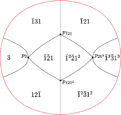
(a) $G_{2}$

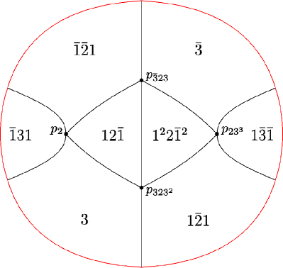
(b) $G_{2}^{-1}$

Figure 3. The combinatorics of the face corresponding to $G_{2}$ and $G_{2}^{-1}$; all 2-faces are labelled, except for the boundary at infinity, which is a disk bounded by the most exterior curve (shown in red). We also label the finite vertices, namely for $w\in\Gamma$, $p_{w}$ denotes being the isolated fixed point of the group element corresponding to the word $w$ ($1=G_{1}$, $2=G_{2}$, $3=G_{3}$, $\bar{1}=G_{1}^{-1}$, etc).

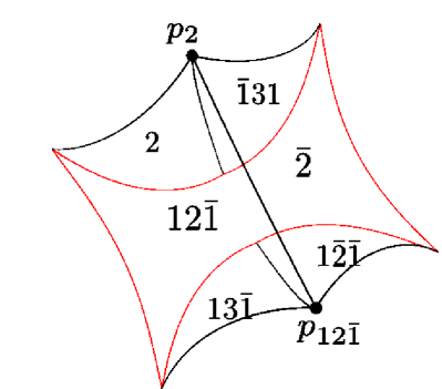
(a) $G_{3}$

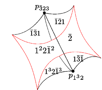
(b) $G_{3}^{-1}$

Figure 4. The combinatorics of the face corresponding to $G_{3}$ and $G_{3}^{-1}$.

We also give a list of vertices on the core sides, and also a list of the bounding bisectors that each vertex lies on, see Tables 1 and 2.

Word	bounding bisectors	Indices
$2$	$2,\bar{2},3,12\bar{1},\bar{1}\bar{2}1,\bar{1}31$	1,2,3,5,10,11
$\bar{1}21$	$2,\bar{1}21,\bar{1}\bar{2}1,\bar{1}31,\bar{1}^{2}\bar{2}1^{2},\bar{1}^{2}31^{2}$	1,9,10,11,18,19
$21^{3}$	$2,\bar{1}21,\bar{1}^{2}\bar{2}1^{2},\bar{1}^{2}\bar{3}1^{2},\bar{1}^{3}\bar{2}1^{3},\bar{1}^{3}\bar{3}1^{3}$	1,9,18,20,26,28
$121^{2}$	$2,12\bar{1},\bar{1}\bar{2}1,\bar{1}\bar{3}1,\bar{1}^{2}\bar{2}1^{2},\bar{1}^{2}\bar{3}1^{2}$	1,5,10,12,18,20

Table 1. Finite vertices on the face for $G_{2}$. For each vertex $v$, we give a word $w$ for an element that fixes precisely $v$, and list the words for the bounding bisectors that contain $v$.

Word	bounding bisectors	Indices
$2$	$2,\bar{2},3,12\bar{1},\bar{1}\bar{2}1,\bar{1}31$	1,2,3,5,10,11
$\bar{3}23$	$\bar{2},\bar{3},12\bar{1},\bar{1}\bar{2}1,\bar{1}\bar{3}1,1^{2}2\bar{1}^{2}$	2,4,5,10,12,13
$23^{3}$	$\bar{2},\bar{3},1\bar{2}\bar{1},1\bar{3}\bar{1},1^{2}2\bar{1}^{2},1^{3}2\bar{1}^{3}$	2,4,6,8,13,21
$323^{2}$	$\bar{2},3,12\bar{1},1\bar{2}\bar{1},13\bar{1},1^{2}2\bar{1}^{2}$	2,3,5,6,7,13

Table 2. Finite vertices on the face for $G_{2}^{-1}$.

Figure 5. The combinatorics at infinity of the fundamental domain, near the faces for $G_{2}^{\pm}$ and $G_{3}^{\pm}$, which are representatives of all faces modulo the action of $G_{1}$.

5.2. Effective local finiteness

The goal of this section is to show that a given face of the Ford domain intersects only finitely many faces. Since the domain is by construction $G_{1}$-invariant, we start by normalizing $G_{1}$ in a convenient form. We will work in the Siegel half space, see section 3.2.

A natural set of coordinates is obtained by arranging that $G_{2}^{2}$ maps $p_{\infty}$ to the origin in the Heisenberg group. There is a unique Heisenberg translation that achieves this, given by

$$Q=\left(\begin{matrix}1&\frac{3-i\sqrt{7}}{4}&-\frac{1}{2}\\ 0&1&\frac{-3-i\sqrt{7}}{4}\\ 0&0&1\end{matrix}\right).$$

One then gets

$$QG_{1}Q^{-1}=\left(\begin{matrix}1&1&-\frac{1}{2}\\ 0&1&-1\\ 0&0&1\end{matrix}\right),$$

and

$$QG_{2}^{2}Q^{-1}=\left(\begin{matrix}0&0&-\frac{1}{2}\\ 0&-1&0\\ -2&0&0\end{matrix}\right).$$

Of course one could make the last matrix even simpler by composing with a loxodromic element.

We denote by $A_{j}=QG_{j}Q^{-1}$. We then have

$$A_{2}(\infty)=(\alpha,0),\quad A_{2}^{2}(\infty)=(0,0),\quad A_{2}^{-1}(\infty)=(-\alpha,0)$$

where $\alpha=\frac{3+i\sqrt{7}}{4\sqrt{2}}$.

$$A_{3}(\infty)=(-\frac{1}{2\sqrt{2}},-\frac{\sqrt{7}}{8}),\quad A_{3}^{-1}(\infty)=(-\frac{1}{\sqrt{2}},\frac{\sqrt{7}}{2}).$$

The spinal sphere with center $(0,0)$ and radius $r$ has equation

(20) $$(x^{2}+y^{2})^{2}+t^{2}=r^{4},$$

so we get a spinal sphere centered at $(a+ib,u)$ by translation:

(21) $$\left((x-a)^{2}+(y-b)^{2}\right)^{2}+(t-u-ay-bx)^{2}=r^{4}.$$

By writing out the equation (7), squaring both sides and identifying with equation (21), one checks that the spheres $\mathcal{S}_{1}$, $\mathcal{S}_{2}$ have radius $1$, whereas $\mathcal{S}_{3}$, $\mathcal{S}_{4}$ have radius $2^{-1/4}$. We summarize this information in Table 3.

Sphere	Center	radius
$\mathcal{S}_{1}$	$(\frac{3+i\sqrt{7}}{4\sqrt{2}},0)$	$1$
$\mathcal{S}_{2}$	$(-\frac{3+i\sqrt{7}}{4\sqrt{2}},0)$	$1$
$\mathcal{S}_{3}$	$(-\frac{1}{2\sqrt{2}},-\frac{\sqrt{7}}{8})$	$2^{-1/4}$
$\mathcal{S}_{4}$	$(-\frac{1}{\sqrt{2}},\frac{\sqrt{7}}{2})$	$2^{-1/4}$

Table 3. Centers and radii of core spinal spheres.

The action of $A_{1}$ on the Heisenberg group is given by

(22) $$(z,t)\mapsto(z-1,t+\Im(z)),$$

and in particular we get the following:

Proposition 5.2.

The element $A_{1}$ preserves every $\mathbb{R}$-circle of the form $(x,0,t_{0})$, $x\in\mathbb{R}$.

Recall that $\mathbb{R}$-circles are by definition given by the trace at infinity of totally geodesic copies of $H^{2}_{\mathbb{R}}$ in $H^{2}_{\mathbb{C}}$. The corresponding real planes in $H^{2}_{\mathbb{C}}$ are preserved by $A_{1}$, and their union is the so-called invariant fan of $A_{1}$ (see [16]).

Among all these $\mathbb{R}$-circles, the $x$-axis is somewhat special because of the following:

Proposition 5.3.

The $\mathbb{R}$-plane bounded by the $x$-axis contains the fixed point of $G_{2}$.

Indeed, the fixed point of $A_{2}$ is given by

$$V=(-\frac{1}{2},0,1),$$

and for $W=(-x^{2}+it,x\sqrt{2},1)$,

$$\langle V,p_{\infty}\rangle\langle p_{\infty},W\rangle\langle W,V\rangle=-\frac{1}{2}(1+x^{2})+it$$

which is real if and only if $t=0$.

Note that equation (22) shows that for any two bisectors $\mathcal{B}_{1}$ and $\mathcal{B}_{2}$ not containing $p_{\infty}$, $G_{1}^{k}\mathcal{B}_{1}\cap\mathcal{B}_{2}=\emptyset$ whenever $k$ is large enough. Indeed, it follows from the detailed study of bisector intersection in [14] that, if two bisectors intersect, then the corresponding spinal spheres must intersect.

Moreover, this claim can easily be made effective, i.e. one can get explicit bounds on how large $k$ needs to be for the above intersection to be empty. If $\mathcal{S}_{j}=\partial_{\infty}\mathcal{B}_{j}$ is contained in a strip $\alpha_{j}\leq x\leq\beta_{j}$, one can simply take $k>\beta_{2}-\alpha_{1}$, or $k<\alpha_{2}-\beta_{2}$. Note that bounds $\alpha_{j},\beta_{j}$ can be computed fairly easily from the equations of the relevant spinal spheres (see the Table 3 giving the centers and radii).

In particular, we get:

Proposition 5.4.

$\mathcal{S}_{1}$ intersects $G_{1}^{k}\mathcal{S}_{1}$ only if $-2\leq k\leq 2$; $\mathcal{S}_{1}$ intersects $G_{1}^{k}\mathcal{S}_{2}$ only if $-4\leq k\leq 1$;

$\mathcal{S}_{1}$ intersects $G_{1}^{k}\mathcal{S}_{3}$ only if $-3\leq k\leq 1$; $\mathcal{S}_{1}$ intersects $G_{1}^{k}\mathcal{S}_{4}$ only if $-4\leq k\leq 0$.

$\mathcal{S}_{2}$ intersects $G_{1}^{k}\mathcal{S}_{2}$ only if $-2\leq k\leq 2$; $\mathcal{S}_{2}$ intersects $G_{1}^{k}\mathcal{S}_{3}$ only if $-2\leq k\leq 2$;

$\mathcal{S}_{2}$ intersects $G_{1}^{k}\mathcal{S}_{4}$ only if $-2\leq k\leq 2$; $\mathcal{S}_{3}$ intersects $G_{1}^{k}\mathcal{S}_{3}$ only if $-2\leq k\leq 2$;

$\mathcal{S}_{3}$ intersects $G_{1}^{k}\mathcal{S}_{4}$ only if $-2\leq k\leq 1$; $\mathcal{S}_{4}$ intersects $G_{1}^{k}\mathcal{S}_{4}$ only if $-2\leq k\leq 2$;

This is not an optimal result, since it takes into account only the variable $x$ and the fact that $G_{1}$ translates by one unit in the direction of the $x$-axis. The optimal result is not far from this though, the point of Proposition 5.4 is to get down to a finite list of bounding bisectors intersecting a given one (so that we can use effective computational tools). We will give much more precise information in the next section.

5.3. Proof of the combinatorics

The techniques we use in order to justify the combinatorics are very similar to the ones explained in detail in [7] and [8]. Note that one can think of justifying the combinatorics as a special case of finding the connected components of (many) semi-algebraic sets. Indeed, $F$ is clearly semi-algebraic, defined by inequalities, indexed by $I=\mathbb{N}$:

$$F=\{z\in\mathbb{C}^{2}\ :\forall i\in I,\ f_{i}(z)<0\},$$

For convenience, we make the convention that $f_{0}(z)<0$ is the defining equation for the unit ball, in other words

$$f_{0}(z)=\langle\tilde{z},\tilde{z}\rangle,$$

where $\tilde{z}=(z,1)$. In particular, we consider the boundary at infinity of complex hyperbolic space as a bounding face. All other equations have the form $f_{j}<0$ where

$$f_{j}(z)=|\langle\tilde{z},\tilde{p}_{0}\rangle|^{2}-|\langle\tilde{z},\gamma_{j}\tilde{p}_{0}\rangle|^{2}.$$

The facets are of $F$ described by taking some subset $J\subset I$, and replacing the inequalities indexed by elements of $J$ by the corresponding equality:

$$F_{J}=\{z\in\mathbb{C}^{2}\ :\ \forall j\in J,\ f_{j}(z)=0,\forall i\in I\setminus J,\ f_{i}(z)<0\}.$$

The fact that $I$ is infinite will not be a problem because of the results in section 5.2, which imply that our polytope is be locally finite.

More generally, we will consider sets of the form

$$F_{J,K}=\{z\in\mathbb{C}^{2}\ :\ \forall j\in J,\ f_{j}(z)=0,\forall i\in K,\ f_{i}(z)<0\},$$

where $J$ and $K$ are disjoint. In particular $F_{J}$ is the same as $F_{J,I\setminus J}$, and $F_{J,\emptyset}$ is the $|J|$-fold bisector intersection containing $F_{J}$.

5.3.1. Terminology and specification

We will call $k$-faces the facets of our polytopes that have dimension $k$. Moreover, 3-faces will be simply called sides, 2-faces will be called ridges, 1-faces will be called edges, and 0-faces will be called vertices.

In terms of computations, it will be important to encode vertices. These can be of two kinds, namely they can be of the form $F_{A,\emptyset}$, for some $A$ with $|A|=4$, or they can be singular points of $F_{B,\emptyset}$ with $|B|=3$). In both cases, they can be obtained by solving a 0-dimensional system (this is the content of assumption 5.5). For each of them, we encode the vertex by storing a rational univariate representation for the corresponding solution set, and an isolating interval specifying a root of the rational parameter (see section 5.3.3).

Note that in the above description, the set $A$ is not unique, since a vertex may in general lie on more than four bisectors (see the discussion in section 4.2, where we saw examples of vertices lying on at least six bounding bisectors). Moreover, in general one cannot take $A$ to be just any $4$-tuple of bisectors that contain that vertex, since some intersections may not be generic.

We will also need to encode 1-faces. There are two kinds of 1-faces, namely those that lie in triple bisector intersections (we call these finite 1-faces), and those that lie in the intersection of the sphere at infinity $\partial_{\infty}{{\bf H}^{2}_{\mathbb{C}}}$ with the closure in ${{\overline{\bf H}}^{2}_{\mathbb{C}}}$ of a bisector intersection (we call these ideal 1-faces, or 1-faces at infinity). Computationally, we make no difference between these two kinds of 1-faces, since both kinds are given in terms of spinal coordinates for a bisector intersection by an equation that is quadratic in both variables.

We call an arc a subset in ${{\overline{\bf H}}^{2}_{\mathbb{C}}}$ of a triple bisector intersection (or a subset of the trace at infinity of a double bisector intersection) that is

• homeomorphic to a closed interval,

• parametrized by one of the spinal coordinates, and such that

• its endpoints are vertices of the polytope, but its interior contains no vertex of the polytope.

Note that a 1-face can always be described as a union of finitely many arcs (but one arc may not suffice, think of a polytope that has a whole Giraud disk as a facet, so that the boundary of that Giraud disk is a 1-face homeomorphic to a circle).

We now expand a little on how to parametrize (pieces of) 1-faces by a single coordinate (we discuss only parametrization by $t_{1}$, the other one is entirely similar). Recall from section 3.1 that the relevant defining functions $h(t_{1},t_{2})$ for triple bisector intersections (or trace at infinity of double bisector intersections) have degree at most two in each variable, so we can write them as

$$a_{2}(t_{1})t_{2}^{2}+a_{1}(t_{1})t_{2}+a_{0}(t_{1}),$$

with $a_{j}$ at most quadratic. With respect to projection onto the first coordinate axis, the curve usually has two branches, given by

$$t_{2}=\frac{-a_{1}(t_{1})\pm\sqrt{\Delta(t_{1})}}{2a_{2}(t_{1})},$$

where

$$\Delta(t_{1})=a_{1}(t_{1})^{2}-4a_{2}(t_{1})a_{0}(t_{1}).$$

Specifically, this occurs above intervals of $t_{1}$ such that $a_{2}(t_{1})$ does not vanish. Above such an interval, the “top branch” is obtained by taking $+\sqrt{\Delta}$ when $a_{2}(t_{1})>0$, and $-\sqrt{\Delta}$ when $a_{2}(t_{1})>0$. We call the other branch the “bottom branch”.

If $a_{2}$ is identically zero, then the curve is either empty, or consists of a single vertical line (so branches above the $t_{1}$ axes are undefined, and there is a single branch with respect to the projection onto the $t_{2}$ axis).

If $a_{2}$ is not identically zero, it vanishes at one or two points, and above each of these points, one can determine check whether the curve contains one, two or infinitely many points (one needs to determine whether $a_{1}$, $a_{0}$ also vanish at these points).

5.3.2. General procedure

The pictures in Section 5.1 include the statement that each facet is topologically (in fact piecewise smoothly) a disk with piecewise smooth boundary (with pieces of the boundary corresponding to facets of codimension one higher). This is not at all obvious; one of the difficulties is the fact that the sets $F_{J}$ are in general not connected, in strong contrast with Dirichlet or Ford domains in the context of constant curvature geometries (see the discussion in [5]).

For a given $J$, $K$, there is an algorithm to decide whether $F_{J,K}$ is empty or not, and furthermore one can list its connected components (and even produce triangulations). One possible approach to this is the cylindrical algebraic decomposition of semi-algebraic sets, see [2] for instance.

The main issue when using such algorithms is that the number of semi-algebraic sets to study is extremely large. If $F$ has $N$ faces, in principle one has to deal with $N\choose k$ potential facets of codimension $k$, where $k=1,2,3,4$, which is a fairly large number of cylindrical decompositions. Rather, we will bypass the cylindrical decomposition and use as much geometric information as we can in order to restrict the number of verifications. Also, rather than using affine coordinates in $\mathbb{C}^{2}$, we use natural parametrizations for bisector intersections, deduced from spinal coordinates (see section 3.1).

Going back to geometry, the inequality defining complex hyperbolic space in $\mathbb{C}^{2}$ (which corresponds to $f_{0}$) is of course a bit different from the other inequalities. In particular, when using the notation $F_{J,K}$, we will always assume one of the index sets $J$ or $K$ contains $0$.

If $K$ contains $0$, then by definition $F_{J,K}$ is contained in ${{\bf H}^{2}_{\mathbb{C}}}$; we will denote by $\widehat{F}_{J,K}$ its extension to projective space, namely

$$\widehat{F}_{J,K}=F_{J,K\setminus\{0\}}.$$

We will also refer to the following set as the trace at infinity of $F_{J,K}$,

$$\partial_{\infty}F_{J,K}=F_{J\cup\{0\},K\setminus\{0\}}.$$

By $\overline{F}_{J,K}$, we mean the set obtained from the definition of $F_{J,K}$ by replacing $<$ by $\leq$, i.e.

$$\overline{F}_{J,K}=\{z\in\mathbb{C}^{2}\ :\ \forall j\in J,\ f_{j}(z)=0,\forall i\in K,\ f_{i}(z)\leq 0\},$$

which is also

$$\overline{F}_{J,K}=\bigcup_{L\subset K}F_{J\cup L,K\setminus L}.$$

Note that in general, this is not the closure of $F_{J,K}$ in $\mathbb{C}^{2}$.

We focus on an algorithm for determining the combinatorics of ridges, or in other words facets of the form $F_{J}$ with $|J|=2$. In most cases, we will also assume $0\notin J$, i.e. we study finite facets rather than faces in $\partial_{\infty}{{\bf H}^{2}_{\mathbb{C}}}$. The algorithm will produce a description of the facets in $\partial F_{J}$, so we get a list of the 1- and 0-faces along the way. The 3-faces are easily deduced from the 2-faces.

The basis for our analysis is the following, which follows from the theory of Gröbner bases (see [4] for instance, and also section 5.3.3 of the present paper). Let $\ell$ be a number field.

• There is an algorithm to determine whether a system of $n$ polynomial equations defined over $\ell$ in $n$ unknowns is 0-dimensional (i.e. whether there are only finitely many solutions in $\mathbb{C}^{n}$);

• If the system is indeed 0-dimensional, there is an algorithm to determine the list of solutions; their entries lie in a finite extension $k\supset\ell$. One can also determine the list of rational/real solutions.

• Polynomials with coefficients in $\ell$ can be evaluated at the solutions of a point with coordinates in $k$, and one can determine whether the value is positive (resp. negative or zero).

When such systems have solution sets with unexpectedly high dimension, there is usually a geometric explanation (typically some of the intersecting bisectors share a slice, see [8] for instance). We will not address this issue, since it never occurs in the situation of the present paper.

In all situations we will consider here, the extension $\ell$ will a quadratic number field, and $k$ will have degree at most four over $\ell$. This makes all computations very quick (using capabilities of recent computers, and standard implementations of Gröbner bases).

For the rest of the discussion, we make the following assumptions.

Assumption 5.5.

1. For every $L\subset I$ with $|L|=4$, $F_{L}$ has dimension zero.

2. For every $J\subset I$ with $|J|=2$, and every $x\in I$, $x\notin J$, the restriction $g_{x}$ of $f_{x}$ to $F_{J,\emptyset}$ has non-degenerate critical points.

These assumptions are by no means necessary in order to determine the combinatorial structure of $F_{J,K}$, but they will simplify the discussion in several places. Note also that they can be checked efficiently using a computer, in particular we state

Proposition 5.6.

Let $M$ be the figure eight knot complement. Then the Ford domain of the irreducible boundary unipotent representation $\rho:\pi_{1}(M)\rightarrow PU(2,1)$, centered at the fixed point of the holonomy of any peripheral subgroup satisfies assumption 5.5.

In contrast, the domains that appear in [8] do not satisfy these hypotheses.

The combinatorial description of $F_{J}$ (i.e. its connected components, and the list of facets adjacent to it) can be obtained by starting from a description of $F_{J,\emptyset}$, and repeatedly studying $F_{J,K\cup\{x\}}$ from $F_{J,K}$, where $x\in I$ is not in $J\cup K$. The latter inductive step is done as follows.

The boundary $\partial F_{J,K}$ can be described as a union of arcs contained in $F_{J\cup\{k\},K\setminus\{k\}}$ for some $k\in K$. For computational purposes, we will always assume that an arc is homeomorphic to a closed interval, that its endpoints are vertices, but none of its interior points are vertices.

Note also that the arcs may not be equal to $F_{J\cup\{k\},K\setminus\{k\}}$, since $F_{J\cup\{x\},\emptyset}$ may have a double point.

For each arc $a$ in $\partial F_{J,K}$ as above, we study the set

$$F_{J\cup\{k,x\}},$$

which by assumption 5.5(1) is obtained by solving a 0-dimensional system. Keeping only solutions that lie in $a$, we get a subdivision of $a$ into connected components of $a\setminus F_{J\cup\{k,x\}}$, and for each such component we check whether or not it is in $F_{J\cup\{k\},\{x\}}$. If so, it is a component of the boundary of $F_{J,K\cup\{x\}}$.

We then compute the critical points of the restriction to $F_{J}$ of the equation $f_{x}$ (this can be done because of assumption 5.5(2), and determine whether any such critical point is inside $F_{J,K}$.

Suppose $c$ is in a component $C_{J,K}$ of $F_{J,K}$.

• If $g_{x}(c)=0$ and $c$ is a saddle point for the restriction $g_{x}$ of $f_{x}$, then a neighborhood of $c$ in $\overline{F}_{J,K\cup\{x\}}$ is the union of two sectors meeting in their apex. In a neighborhood of $c$, $F_{J,K\cup\{x\}}$ will have four boundary arcs. Each such arc will either connect $c$ to another saddle point of $g_{x}$, or it will connect it to a vertex in the boundary of $C_{J,K}$. For each such arc, we take a sample point to check whether it is contained in $F_{J\cup\{x\},K}$.

• If $g_{x}(c)\neq 0$, there could be an isolated component of $F_{J\cup\{x\},K}$ that winds around $c$. In order to determine whether this happens or not, we consider the slice $t_{1}=\alpha_{1}$, and intersect it with $g_{x}=0$. Recall that this intersection contains either 0, 1, or 2 points (because it is obtained by solving an equation that has degree at most two, which is not identically zero because $g_{x}(c)\neq 0$).

  Then there is an isolated component if and only if the intersection consists of precisely two points, and the two intersection points lie in the same connected component of $F_{J,K}$.

Now collecting the boundary arcs with the inside arcs (joining two points that are either saddle or boundary vertices $F_{J\cap\{k,x\}}$), we get a stratum decomposition for $F_{J,K\cup\{x\}}$.

Moreover, if we make the following assumption, then all components of $F_{J,K\cup\{x\}}$ are topological disks, since their boundary consists of a single component.

Assumption 5.7.

1. The curves $F_{J\cup\{x\},K}$ do not have any isolated component in $F_{J,K}$.

Once again, in the special case of the Ford domain relevant to the irreducible boundary unipotent rank one, it turns out this hypothesis is satisfied.

5.3.3. Rational Univariate Representation

We briefly recall what we need about rational univariate representations; for details on this technique, see [24]. Recall that given a 0-dimensional polynomial system

(23) $$\left\{\begin{array}[]{l}f(t_{1},t_{2})=0\\ g(t_{1},t_{2})=0\end{array}\right.$$

with coefficients in the number field $\ell$, we can write it as a polynomial system with rational coefficients by using a primitive element for $\ell$; the corresponding system has one more variable (which we denote by $s$), and one more equation (which is the minimal polynomial of a primitive generator for $\ell$). We write it in the form

(24) $$\left\{\begin{array}[]{l}\tilde{f}(t_{1},t_{2},s)=0\\ \tilde{g}(t_{1},t_{2},s)=0\\ m(s)=0\end{array}\right.$$

where $\tilde{f}$ is obtained from $f$ by expressing its coefficients as polynomials in the primitive element for $\ell$. In the cases that interest us, $\ell$ will be a totally real number field, which we assume from now on.

In this discussion we consider systems of two equations in two variables (so we get 3 equations in 3 variables, counting the extra-variable corresponding to the primitive element of the number field), but we could also allow system that have more equations than the number of variables (the important point is that the ideal generated by the equations should be 0-dimensional).

Now the key point is that there exists a 1-variable polynomial $r$ such that the solutions are parametrized as rational functions of the roots of $r$. More specifically, there exist polynomials $r$, $p_{0}$, $p_{1}$, $p_{2}$ and $q$ with integer coefficients such that the solutions of the system can be written in the form

(25) $$s=p_{0}(u)/q(u),t_{1}=p_{1}(u)/q(u),\quad t_{2}=p_{2}(u)/q(u),$$

and the latter formula gives a solution of (24) if and only $u$ is a root of $r$. Of course, since in general the minimal polynomial $m$ has several roots, this produces more solutions of system (23) than we would like. The solutions of (23) can easily be obtained by sifting the solutions of (24) once we know isolating intervals for the roots of $m$.

Note that, even though all the equations relevant to this paper have coefficients in a fixed number field (namely $\ell=\mathbb{Q}(\sqrt{7})$), the vertices usually have entries in a larger number field (namely the field generated by a given root of the rational parametrizing polynomial $r$).

Note also that the solutions lie in a subfield $L\subset\mathbb{C}$ if and only if the corresponding root $u$ of $r$ lies in $L$. In particular, if we want to find real solutions of the system, we can restrict to studying real roots of $r$, which can be specified by isolating intervals.

Using a rational univariate representation for the vertices provides a convenient set of methods that allow us to:

1. find the list of faces that contain a given vertex;

2. for each bounding bisector not containing a vertex, check which side the vertex is in;

3. check if two vertices are the same;

4. check whether a given vertex is inside a given arc;

5. if two vertices in $F_{J\cup\{x\},\emptyset}$ are given, check whether these two vertices are joined by an arc in $F_{J\cup\{x\},\emptyset}$.

Items (i) and (ii) are very simple because all our equations are defined over a given $\ell$. Given a polynomial $h(t_{1},t_{2})=\tilde{h}(t_{1},t_{2},s)$, we start by substituting the parametrization (25) in $\tilde{h}$, replacing $u$ by the appropriate interval of values of the rational parameter. If the corresponding interval does not contain 0, we know the sign of $h$ at that vertex.

Otherwise, we keep the exact parametrization (25) and get a rational function in $u$ that represents $h$ at the solutions of (24), and we check whether it vanishes at the appropriate root of $r$. This corresponds to checking whether our favorite root of the rational parametrizing polynomial $r$ is also a root of another given polynomial with integer coefficients (namely the numerator of the above rational function); this can be done by computing their greatest common divisor, and isolating its real roots.

If the rational function does not vanish, we compute a more precise interval for the value of $\tilde{h}$, and refine precision untill the interval does not contain 0. Of course, in all generality, this may require such high precision that it would exhaust the system memory, but this does not seem to happen for the verifications that appear in this paper, at least for our implementation on standard modern computers.

We now sketch how to implement item (iii). Suppose we are given two rational parametrizations

$$\begin{array}[]{l}s=p_{0}(u)/q(u),t_{1}=p_{1}(u)/q(u),\quad t_{2}=p_{2}(u)/q(u)\\ s=a_{0}(v)/b(v),t_{1}=a_{1}(v)/b(v),\quad t_{2}=a_{2}(v)/b(v),\end{array}$$

where $u$ (resp. $v$) is to be taken to be a specific root of $r(u)$ (resp. $c(v)$). Equality corresponds to verifying whether $p_{1}(u)b(v)-q(u)a_{1}(v)$ (resp. $p_{2}(u)b(v)-q(u)a_{2}(v)$) vanishes at the corresponding roots. If the rational parameters were the same, this would simply amount to computing a greatest common divisor, but in general the parameters from both rational representaions are different.

One way to handle this is to solve the system

$$\left\{\begin{array}[]{l}p_{1}(u)b(v)-q(u)a_{1}(v)=0\\ r(u)=0\\ c(v)=0\end{array}\right.,$$

which can be done using a rational univariate representation once again. The result then follows from sifting solutions and keeping only those that give the right root for $u$ and $v$, and checking whether the sift gives a solution of not.

In order to explain how to check (iv), we need to describe in more detail how we encode arcs. We will assume

• that every arc is parametrized by one of the spinal coordinates (this can always be achieved, perhaps after subdividing certain arcs if necessary),

• that the endpoints of every arc are vertices (parametrized by a rational univariate representation, as discussed above), and

• that there are no vertices stricly inside any arc.

Then, in order to check whether a given vertex is inside an arc parametrized by $t_{1}$, we need to compare its $t_{1}$ value with the $t_{1}$ values of the endpoints of the arc. This amounts to checking the sign of an expression of the form

$$p_{1}(u)/q(u)-a_{1}(v)/b(v),$$

where $u$ (resp. $v$) is a specific root of $r$ (resp. $c$). This is the same as the test that occurs in item (iii).

If the vertex $t_{1}$ value is between the $t_{1}$-values of the endpoints of the arc, we still need to check whether it is in the correct arc.

5.3.4. Sample computations

We determine some sets $F_{J}$, $|J|=2$ explicitly, in order to illustrate the phenomena that can occur when applying the algorithm from the previous section. The general scheme to parametrize $F_{J,\emptyset}$ is explained in [7], for instance.

When $0\notin J=\{j,k\}$, we distinguish two basic cases, depending on whether $p_{0}$, $p_{j}$ and $p_{k}$ are in a common complex line. This happens if and only if some/any lifts $\tilde{p}_{j}\in\mathbb{C}^{3}$ are linearly dependent. In that case, the bisectors $F_{\{j\}}$ and $F_{\{k\}}$ have the same complex spine, and their intersection is either empty or a complex line (this never happens in the Ford domains studied in this paper).

Otherwise, $F_{J,\emptyset}$ can be parametrized by vectors of the form

$$(\bar{z}_{1}p_{0}-p_{j})\boxtimes(\bar{z}_{2}p_{0}-p_{k})=z_{1}p_{k0}+z_{2}p_{0j}+p_{jk},$$

with $|z_{1}|=|z_{2}|=1$, and where $p_{mn}$ denotes $p_{m}\boxtimes p_{n}$ (see section 3.1).

Valid pairs $(z_{1},z_{2})$ in the Clifford torus $|z_{1}|=|z_{2}|=1$ are given by pairs where

$$\langle z_{1}p_{k0}+z_{2}p_{0j}+p_{jk},z_{1}p_{k0}+z_{2}p_{0j}+p_{jk}\rangle<0,$$

which can be rewritten as

$$\Re(\mu_{0}(z_{1})z_{2})=\nu_{0}(z_{1}),$$

for $\mu_{0}$ and $\nu_{0}$ affine in $z_{1},\bar{z}_{1}$.

In terms of the notations of section 5.3.2, the restriction $g_{0}$ of $f_{0}$ to $F_{J,\emptyset}$ is given by

$$g_{0}(z_{1},z_{2})=\Re(\mu_{0}(z_{1})z_{2})-\nu_{0}(z_{1})).$$

In order to draw pictures, we will sometimes use log-coordinates $(t_{1},t_{2})$ for $F_{J,\emptyset}$, and write, for $j=1,2$,

$$z_{j}=exp(2\pi it_{j}).$$

Given $l\notin J$, we already mentioned in section 3.1 how to write the restriction $g_{l}$ of $f_{l}$ to to $F_{J}$. Note that $\langle p_{k0},p_{0}\rangle=\langle p_{0j},p_{0}\rangle=0$, so the equation $f_{x}$ reads

$$|\langle p_{jk},p_{0}\rangle|=|\langle z_{1}p_{k0}+z_{2}p_{0j}+p_{jk},p_{l}\rangle|,$$

which again can be written in the form

$$\Re(\mu_{l}(z_{1})z_{2})=\nu_{l}(z_{1}).$$

In order to compute the critical points of the restriction to $|z_{1}|=|z_{2}|=1$ of a function $h(z_{1},\bar{z}_{1},z_{2},\bar{z}_{2})$, we search for points where

$$\left\{\begin{array}[]{l}\frac{\partial h}{\partial z_{1}}z_{1}-\frac{\partial h}{\partial\bar{z}_{1}}\bar{z}_{1}=0\\ \frac{\partial h}{\partial z_{2}}z_{2}-\frac{\partial h}{\partial\bar{z}_{2}}\bar{z}_{2}=0\end{array}\right.,$$

Gröbner bases for the corresponding systems tell us whether these critical points are non-degenerate (see assumption 5.7), and if so, we can compute them fairly explicitly, i.e. describe their coordinates as roots of explicit polynomials (in particular they can be computed to arbitrary precision).

Proposition 5.8.

Let $J=\{1,2\}$. Then $F_{J}$ is empty, and $\overline{F}_{J}$ is a singleton, given by $F_{\{1,2,3,5,10,11\}}$.

The singleton in the Proposition is $\{p_{2}\}$, for $p_{2}$ as in Lemma 4.2. It follows from the Proposition that $p_{2}$ lies precisely on six bounding bisectors (Lemma 4.2 only showed that it was on at least six, listed in Tables 1 and 2).

Proof: For $J=\{1,2\}$, we get

$$\mu_{0}(z_{1})=-2-\bar{z}_{1},\quad\nu_{0}(z_{1})=-3+z_{1}+\bar{z}_{1}.$$

The discriminant

$$|\mu|^{2}-\nu^{2}=-6+16\Re z_{1}-2\Re z_{1}^{2}$$

vanishes precisely for four complex values of $z_{1}$, which are the roots of

(26) $$z_{1}^{4}-8z_{1}^{3}+6z_{1}^{2}-8z_{1}+1.$$

Since we know $F_{J,\{0\}}$ is connected (see [14], Theorem 9.2.6), we know that at most two of these roots lie on the unit circle. In fact, $z_{1}=z_{2}=1$ gives a point in $F_{J,\{0\}}$, so $F_{J,\{0\}}$ is non empty, hence there must be two (complex conjugate) roots on the unit circle. Indeed, these roots have argument $2\pi t$ with $t=\pm 0.20682703\dots$.

A more satisfactory way to check that the polynomial (26) has precisely two roots on the unit cirle is to split $z_{1}=x_{1}+iy_{1}$ into its real and imaginary parts (this gives a general method that does not rely on geometric arguments).

Indeed $z_{1}$ is a root of (26) if and only if $(x_{1},y_{1})$ is a solution of the system $-6+16x_{1}-2x_{1}^{2}+2y_{1}^{2}=0$, $x_{1}^{2}+y_{1}^{2}=1$. These equations imply that $x_{1}=2\pm\sqrt{3}$, and then

$$y_{1}^{2}=2-4x_{1},$$

which is positive only for $x_{1}=2-\sqrt{3}$, and then we get $y_{1}=\pm\sqrt{4\sqrt{3}-6}$.

In order to run the algorithm from the preceding section, we write the restriction $g_{3}$ of $f_{3}$ to $F_{J,\emptyset}$, which is given by

$$-3+2\Re\{\frac{1-i\sqrt{7}}{2}z_{1}+\frac{5-i\sqrt{7}}{2}z_{2}+\frac{-3+i\sqrt{7}}{2}z_{1}\bar{z}_{2}\}.$$

Gröbner bases calculations show that the system $g_{0}(z)=g_{3}(z)=|z_{1}|^{2}-1=|z_{2}|^{2}-1=0$ has precisely two solutions, given in log-coordinates by

$$(-0.20418699\dots,-0.03294828\dots),\quad(0.15576880\dots,-0.07655953\dots).$$

Once again, the most convenient way to use Gröbner bases is to work with four variable $x_{1},y_{1},x_{2},y_{2}$ given by real and imaginary parts of $z_{1}$ and $z_{2}$ (with extra equations $x_{j}^{2}+y_{j}^{2}=1$.

The combinatorics of $F_{J,K}$ for $K=\{0,3\}$ are illustrated in Figure 6(b). It is a disk with two boundary arcs, given by $F_{\{1,2,0\},\{3\}}$ and $F_{\{1,2,3\},\{0\}}$.

(a) $F_{\{1,2\},\{0\}}$

(b) $F_{\{1,2\},\{0,3\}}$

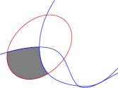
(c) $F_{\{1,2\},\{0,3,5\}}$

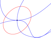
(d) $F_{\{1,2\}}$

Figure 6. Steps of the algorithm to determine $F_{\{1,2\}}$.

As the next element to include in $K$, we choose 5 rather than 4, in order to shorten the discussion slightly. The curve $F_{\{1,2,5\},\emptyset}$ intersects $F_{\{1,2,0\},\emptyset}$ two points, given in log-coordinates by

$$(0.04600543\dots,0.20593006\dots),\quad(0.05483483\dots,-0.17019919\dots).$$

Only the second one is inside the arc $F_{\{1,2,0\},\{3\}}$.

The curve $F_{\{1,2,5\},\emptyset}$ intersects $F_{\{1,2,3\},\emptyset}$ in five points, given by $(z_{1},z_{2})=$

$$(1,1),\ (i,-i),\ (-i,i),(\frac{9+5i\sqrt{7}}{16},\frac{-3+i\sqrt{7}}{4}),\ (\frac{-3+i\sqrt{7}}{4},\frac{1-3i\sqrt{7}}{8}).$$

only one of which is in $F_{\{1,2,3\},\{0\}}$, namely $(1,1)$.

Now $F_{\{1,2\},\{0,3,5\}}$ has three boundary arcs, given by $F_{\{1,2,0\},\{3,5\}}$, $F_{\{1,2,3\},\{0,5\}}$ and $F_{\{1,2,5\},\{0,3\}}$ (see Figure 6(c)).

Next, we include 10 in $K$. The curve $F_{\{1,2,10\},\emptyset}$ intersects $F_{\{1,2,0\},\emptyset}$ in two points, none of which is in $F_{\{1,2,0\},\{3,5\}}$. Hence the arc $F_{\{1,2,0\},\{3,5\}}$ is either completely inside, or completely outside $F_{\{1,2,0\},\{3,5,10\}}$. One easily checks that it is outside, by taking a sample point.

The curve $F_{\{1,2,10\},\emptyset}$ intersects $F_{\{1,2,3\},\emptyset}$ in five points, none of which is in $F_{\{1,2,3\},\{0,5\}}$. The arc $F_{\{1,2,3\},\{0,5\}}$ is either completely inside, or completely outside $F_{\{1,2,3\},\{0,5,10\}}$ and a sample point shows it is outside.

Similarly, the curve $F_{\{1,2,10\},\emptyset}$ intersects $F_{\{1,2,5\},\emptyset}$ in six points, none of which is in $F_{\{1,2,5\},\{0,3\}}$, and the arc $F_{\{1,2,5\},\{0,3\}}$ is completely outside $F_{\{1,2,3\},\{0,5,10\}}$.

This implies that $F_{\{1,2\}}$ is empty (see Figure 6(d)).

Finally we consider the intersection of $F_{\{1,2,10\},\emptyset}$ with the three vertices of $F_{\{1,2\},\{0,3,5\}}$. One easily checks that the only intersection is the point with complex spinal coordinates given by $(1,1)$, and this point indeed a vertex of $F$. It is in homogeneous coordinates in $\mathbb{C}^{3}$ given by

$$(\frac{3-i\sqrt{7}}{2},-2,-\frac{3-i\sqrt{7}}{2}),$$

and that it is on precisely six bounding bisectors (by construction it is on $\mathcal{B}_{1}$ and $\mathcal{B}_{2}$, and it is also in $\mathcal{B}_{3}$, $\mathcal{B}_{5}$, $\mathcal{B}_{10}$ and $\mathcal{B}_{11}$). In terms of the notation of section 5.3.2, this point is

$$F_{\{1,2,3,5,10,11\}}.$$

In fact one easily checks that this point is the fixed point of $G_{2}$ (which by definition of the bounding bisectors is obviously in $\mathcal{B}_{1}\cap\mathcal{B}_{2}$). $\Box$

Remark 5.9.

1. Throughout the proof of Proposition 5.8, we have ignored the issue of critical points. In principle, at each stage, we may have missed some isolated components of the curves $F_{\{1,2,k\},\emptyset}$; if this were the case, the set $F_{\{1,2\}}$ would still be contained in the set which we just described, hence it must be empty anyway.

2. The curves $F_{\{1,2,10\},\emptyset}$ and $F_{\{1,2,3\},\emptyset}$ are in fact tangent at $(1,1)$, which is a vertex of $F$. We shall come back to this point later, when discussing stability of the combinatorics of $F$ under deformations.

Proposition 5.10.

$F_{\{1,3\}}$ is combinatorially a triangle, with three boundary arcs given by $F_{\{1,3,0\}}$, $F_{\{1,3,5\}}$, $F_{\{1,3,11\}}$, and three vertices given by $F_{\{0,1,3,5\}}$, $F_{\{0,1,3,11\}}$, and $F_{\{1,2,3,5,10,11\}}$.

Note that this triangle appears in Figure 3(a) and 4(a), it is the intersection of the bounding bisectors $\mathcal{B}_{1}$ (resp. $\mathcal{B}_{3}$) corresponding to $G_{2}$ (resp. $G_{3}$). The edges in ${{\bf H}^{2}_{\mathbb{C}}}$ are on $\mathcal{B}_{5}$, which corresponds to $G_{1}G_{2}G_{1}^{-1}$ and $\mathcal{B}_{11}$, which correspond to $G_{1}^{-1}G_{3}G_{1}$.

Proof: As in the argument for $F_{\{1,2\}}$, we study $F_{J,K}$ for increasing sets $K$, freely choosing the order we use to increase $K$. We describe an efficient way to get down to $F_{\{1,3\}}$ in the form of a picture, see Figure 7.

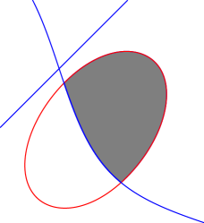
(a) $F_{\{1,3\},\{0,5\}}$

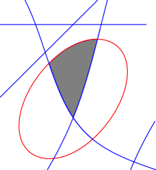
(b) $F_{\{1,3\},\{0,5,11\}}$

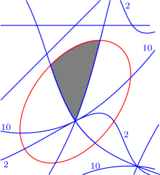
(c) $F_{\{1,3\},\{0,5,11,2,10\}}$

Figure 7. Steps of the algorithm to determine $F_{\{1,3\}}$.

We start by studying $F_{\{1,3\},\{5\}}$. Note that the curve $F_{\{1,3,5\},\emptyset}$ has two double points. These points can be obtained by writing the equation $g_{5}$ as

$$\Re(\mu(z_{1})z_{2})=\nu(z_{1}),$$

where

$$\mu(z_{1})=\frac{3+i\sqrt{7}}{2}-\bar{z}_{1},\quad\nu(z_{1})=1-\Re(\frac{3+i\sqrt{7}}{2}z_{1}).$$

The discriminant $|\mu(z_{1})|^{2}-\nu(z_{1})^{2}$ is given by

$$2+\Re\left(\frac{-1-3i\sqrt{7}}{4}z_{1}^{2}\right),$$

which vanishes for $z_{1}=\pm\frac{3-i\sqrt{7}}{4}.$ Plugging this back into the equation $g_{5}$ gives $z_{2}=\mp\frac{3-i\sqrt{7}}{4}.$ One easily checks that $g_{0}(z_{1},z_{2})>0$ for these two double points, i.e. they lie outside complex hyperbolic space.

One checks that $F_{\{1,3,5\},\emptyset}$ intersects $F_{\{1,3,0\},\emptyset}$ in precisely two points (and these intersections are transverse), so we get two arcs in the boundary of $F_{\{1,3\},\{0,5\}}$, namely $F_{\{1,3,5\},\{0\}}$ and $F_{\{1,3,0\},\{5\}}$ (see Figure 7(a)).

In principle, there could be an extra arc in $F_{\{1,3,5\},\{0\}}$, not intersecting $F_{\{1,3,0\},\emptyset}$, so we compute critical points of $g_{5}$. Their are given by solutions of the system

$$\left\{\begin{array}[]{l}\Im\{(\bar{z}_{2}+\frac{3+i\sqrt{7}}{2})z_{1}\}=0\\ \Im\{(\bar{z}_{1}+\frac{3+i\sqrt{7}}{2})z_{2}\}=0\end{array}\right.,$$

that satisfy $|z_{1}|=|z_{2}|=1$.

There are four such critical points, of the form $(\pm\alpha,\pm\alpha)$ where $\alpha=\frac{3-i\sqrt{7}}{4}$ (of course this list includes the double points computed before). The corresponding points are outside $F$, in fact $g_{0}(\pm\alpha,\pm\alpha)>0$.

A similar analysis justifies part (b) of Figure 7, i.e. that $\overline{F}_{\{1,3\},\{0,5,11\}}$ is combinatorially a triangle (with one side on $\partial_{\infty}{{\bf H}^{2}_{\mathbb{C}}}$).

We sketch how to justify that $F_{\{1,3\}}=F_{\{1,3\},\{0,5,11\}}$. For $k=2$ and $k=10$, the curve $F_{\{1,3,k\},\emptyset}$ actually goes through a vertex of $F_{\{1,3\}}=F_{\{1,3\},\{0,5,11\}}$; for $k\neq 0,2,5,10,11$, $F_{\{1,3,k\},\emptyset}$ does not intersect even $\overline{F}_{\{1,3\},\{0,5,11\}}$.

We start by studying $F_{\{1,3,0\},\emptyset}\cap F_{\{1,3,2\},\emptyset}$. In order to use standard root isolation methods, we use real equations, in $x_{1},y_{1},x_{2},y_{2}$. Computing a Gröbner basis for the ideal generated by the equations $g_{0}$, $g_{3}$, $x_{1}^{2}+y_{1}^{2}-1$ and $x_{2}^{2}+y_{2}^{2}-1$, we see that it contains

$$39-840\sqrt{7}y_{2}+4088y_{2}^{2}+608y_{2}^{3}\sqrt{7}-9152y_{2}^{4}+1024y_{2}^{5}\sqrt{7}+7168y_{2}^{6},$$

which has precisely two real roots, given approximately by $y_{2}^{(1)}=0.01815877\dots$ and $y_{2}^{(2)}=0.65602473\dots$.

The Gröbner basis also gives an expression for $x_{1},y_{1},x_{2}$ in terms of $y_{2}$, namely

$$x_{1}=\{-4943+16836\sqrt{7}y_{2}-142640y_{2}^{2}+53184y_{2}^{3}\sqrt{7}+72128y_{2}^{4}-75264y_{2}^{5}\sqrt{7}\}/14725,$$

$$y_{1}=\{5058\sqrt{7}+45888y_{2}-112560y_{2}^{2}\sqrt{7}+309472y_{2}^{3}+74432y_{2}^{4}\sqrt{7}-422912y_{2}^{5}\}/14725,$$

$$x_{2}=\{20-21\sqrt{7}y_{2}+16y_{2}^{2}+32y_{2}^{3}\sqrt{7}\}/19.$$

Substituting either value $y_{2}^{(j)}$ gives two points $a^{(j)}=(x_{1}^{(j)},y_{1}^{(j)},x_{2}^{(j)},y_{2}^{(j)})$, $j=1,2$ and we claim that $g_{5}(a^{(1)})>0$ and $g_{11}(a^{(2)})>0$. Clearly this can be checked by simple interval arithmetic, in fact

$$g_{5}(a^{(1)})=3.80716606\dots,g_{11}(a^{(2)})=3.94518313\dots.$$

The analysis of $F_{\{1,3,5\},\emptyset}\cap F_{\{1,3,2\},\emptyset}$ is in a sense simpler, because all the solutions to the corresponding system are defined over $\mathbb{Q}(i,\sqrt{7})$. The system has precisely five solutions, given by

$$\begin{array}[]{c}(i,\frac{1+\sqrt{7}}{4}+i\frac{1-\sqrt{7}}{4}),(-i,\frac{1-\sqrt{7}}{4}-i\frac{1+\sqrt{7}}{4}),\\ (\frac{-3+i\sqrt{7}}{4},\frac{3-i\sqrt{7}}{4}),(\frac{9+5i\sqrt{7}}{16},-\frac{9+5i\sqrt{7}}{16},(1,\frac{3+i\sqrt{7}}{4}).\end{array}$$

Only one of these solutions satisfies $g_{0}\leq 0$, namely the last one (in other words, only one intersection point lies ${{\overline{\bf H}}^{2}_{\mathbb{C}}}$).

Note that we already found one point in $F_{\{1,3,2\},\emptyset}\cap F_{\{1,3,5\},\emptyset}$, namely the fixed point of $G_{2}$ (see the proof of Proposition 5.8).

Similarly, one verifies that $F_{\{1,3,2\},\emptyset}\cap F_{\{1,3,11\},\emptyset}$ contains precisely six points, only one of which gives a point in (the closure of) complex hyperbolic space.

Once again, since we already know one point in this intersection (namely the fixed point of $G_{2}$), we get that $F_{\{1,3,2\},\emptyset}$ with $\partial F_{\{0,1,3,5,11\},\emptyset}$ consists of precisely one point. This implies that $\partial F_{\{0,1,3,5,11\},\emptyset}$ is either completely inside or completely outside $\partial F_{\{0,1,3,5,11,2\},\emptyset}$. It is easy to check that it is inside, by testing a sample point (for instance one of the other vertices of the triangle $\partial F_{\{0,1,3,5,11\},\emptyset}$).

We now show that $F_{\{1,3,2\},\emptyset}$ does not intersect $F_{\{0,1,3,5,11\},\emptyset}$, by computing the critical points of $g_{2}$. There are six critical points, given by

$$\begin{array}[]{c}(-1,-\frac{1+3i\sqrt{7}}{8}),(\frac{3-i\sqrt{7}}{4},\frac{3-i\sqrt{7}}{4}),(\pm \frac{1+i\sqrt{7}}{\sqrt{8}}, \pm\frac{1-i\sqrt{7}}{\sqrt{8}}),\end{array}$$

and one easily checks that none of them is inside $F_{\{0,1,3,5,11\},\emptyset}$. In particular, we get that the minimum value of $g_{3}$ on $\overline{F}_{\{0,1,3,5,11\},\emptyset}$ is $0$, and it is realized precisely at one vertex (namely the fixed point of $G_{2}$).

In other words, we get $F_{\{0,1,3,5,11\},\emptyset}=F_{\{0,1,2,3,5,11\},\emptyset}$, i.e. including the inequality $g_{2}<0$ at this stage has no effect. An entirely similar computation shows that $F_{\{0,1,2,3,5,11\},\emptyset}=F_{\{0,1,2,3,5,10,11\},\emptyset}$.

For all $k\neq 0,1,2,3,5,10,11$, $F_{\{0,1,3,k\},\emptyset}$ does not intersect even the closure $\overline{F}_{\{0,1,2,3,5,11\},\emptyset}$, and one can use arguments as above using interval arithmetic. $\Box$

Similar arguments allow us to handle the detailed study of all the polygons that appear on Figure 3 and 4.

Proposition 5.11.

$F_{\{1,4\},\emptyset}$ is a Giraud disk, which is entirely contained in the exterior of $\mathcal{B}_{5}$. In particular, $F_{\{1,4\}}$ is empty.

Proof: We will prove that $F_{\{5\},\emptyset}$ does not intersect the Giraud torus $\widehat{F}_{\{1,4\},\emptyset}$. In order to see this, we use complex spinal coordinates, and write $g_{5}(z_{1},z_{2})$ for the restriction of $f_{5}$ to the Clifford torus $|z_{1}|=|z_{2}|=1$.

One computes explicitly that

$$g_{5}(z_{1},z_{2})=4+2\Re\{\frac{1+i\sqrt{7}}{2}z_{1}\bar{z}_{2}\}.$$

This is clearly always positive when $|z_{1}|=|z_{2}|=1$.

In other words, the Giraud torus $\widehat{F}_{\{1,4\},\emptyset}$ is entirely outside $F$. $\Box$

Proposition 5.12.

$F_{\{1,6\},\emptyset}$ is empty. The Giraud torus $\widehat{F}_{\{1,6\},\emptyset}$ is completely outside complex hyperbolic space, in other words the bisectors $\mathcal{B}_{1}$ and $\mathcal{B}_{6}$ are disjoint.

Proof: We write the equation of $F_{\{0,1,6\},\emptyset}$ in spinal coordinates for the Giraud torus $F_{\{1,6\},\emptyset}$, which reads

$$g_{0}(z_{1},z_{2})=18-2\Re\{4(z_{1}+z_{2})+z_{1}\bar{z}_{2}\}.$$

Clearly this is non-negative when $|z_{1}|=|z_{2}|=1$, and in that case it is zero if and only if $z_{1}=z_{2}=1$.

In other words, $\widehat{\mathcal{B}}_{1}$ and $\widehat{\mathcal{B}}_{2}$ intersect in a point in ${{\overline{\bf H}}^{2}_{\mathbb{C}}}$. Note that this point is not in the closure of $F$, in fact it is strictly outside the half spaces bounded by $\mathcal{B}_{2}$, $\mathcal{B}_{3}$, $\mathcal{B}_{5}$, $\mathcal{B}_{7}$ and $\mathcal{B}_{11}$. $\Box$

Proposition 5.13.

$F_{\{3,8\}}$ is empty. The Giraud torus $F_{\{3,8\},\emptyset}$ contains a disk in ${{\bf H}^{2}_{\mathbb{C}}}$, but $\overline{F}_{\{3,8\},\{2,6\}}$ is empty.

Proof: The proof is actually very similar to that of Proposition 5.10, but since the corresponding set is empty, we go through some of the details.

The curve $F_{\{3,8,2\},\emptyset}$ intersects $F_{\{3,8,0\},\emptyset}$ in precisely two points, and cuts out a disk in the Giraud disk $F_{\{3,8\},\emptyset}$, so that $F_{\{3,8\},\{0,2\}}$ is a disk with only two boundary arcs.

One then easily verifies that $F_{\{3,8,6\},\emptyset}$ does not intersect $\overline{F}_{\{3,8\},\{0,2\}}$, so $F_{\{3,8\},\{0,2,6\}}$ is either equal to $F_{\{3,8\},\{0,2\}}$ or is empty (one needs to check critical points in order to verify this).

By taking a sample point $z$, and checking $f_{6}(z)>0$, one gets that $F_{\{3,8\},\{0,2,6\}}$ is empty. $\Box$

The study of $\mathcal{B}_{1}\cap\mathcal{B}_{k}$ for various values of $k$ is similar to one of the previous few propositions, we list the relevant arguments in Table 4. When the proof is similar to Proposition 5.11, the indices $l$ listed in brackets indicate that $\mathcal{B}_{1}\cap\mathcal{B}_{k}$ is entirely outside the half space bounded by $\mathcal{B}_{l}$.

The corresponding list of arguments used to study of $\mathcal{B}_{3}\cap\mathcal{B}_{k}$ for various values of $k$ in Table 5.

Note that the arguments for $\mathcal{B}_{2}$ (resp. $\mathcal{B}_{4}$) are of course almost the same as those for $\mathcal{B}_{1}$ (resp. $\mathcal{B}_{3}$), since the corresponding faces are actually paired by $G_{2}$ (resp. $G_{3}$).

Prop 5.4	8, 14-16, 21-25, 29-33, 35
Prop 5.8	2, 12, 19, 26
Prop 5.10	3, 5, 9, 10, 11, 18, 20, 28
Prop 5.11	4[5,10], 7[3], 13[2,5,10], 17[9], 27[9,18], 36[17,28,34]
Prop 5.12	6, 34

Table 4. We list the indices where the arguments of each proposition apply to study $\mathcal{B}_{1}\cap\mathcal{B}_{k}$.

Prop 5.4	16, 17, 22-36
Prop 5.8	10, 13
Prop 5.10	1, 2, 5, 6, 7, 11
Prop 5.11	9[11], 14[7], 15[7], 18[1,10], 19[11], 20[7], 21[6,13]
Prop 5.12	4, 12
Prop 5.13	8

Table 5. We list the indices where the arguments of each proposition apply to study $\mathcal{B}_{3}\cap\mathcal{B}_{k}$.

5.3.5. Genericity

In order study deformations $\rho_{t}$ of the boundary unipotent representation $\rho_{0}:\pi_{1}(M)\rightarrow PU(2,1)$, we will need more information that just the combinatorics.

We will determine the non-transverse bisector intersections, and prove that they remain non-transverse in the family of Ford domains for groups in the 1-parameter family where the unipotent generator becomes twist parabolic.

The basic fact is the following, which follows from the restrictive character of the bounding bisector, namely they are all covertical (because they define faces of a Ford domain).

Proposition 5.14.

Let $J=\{j,k\}$ with $j\neq k$. Then the intersection $F_{\{j\},\emptyset}\cap F_{\{k\},\emptyset}=F_{J,\emptyset}$ is transverse at every point of $F_{J,\emptyset}$.

The analogous statement is not true when $|J|\geq 3$, since $F_{J,\emptyset}$ can have singular points (see Figure 6 for instance). This will not be bothersome in the context of our polyhedron $F$, because of the following.

Proposition 5.15.

Suppose $|J|=3$ and $F_{J}$ is non-empty. Then the corresponding intersection of three bisectors (or two bisectors and $\partial_{\infty}{{\bf H}^{2}_{\mathbb{C}}}$) is transverse at every point of $F_{J}$.

Proof: This follows from the fact that double points of $F_{J,\emptyset}$ occur only away from the face $F_{J}$. Indeed, one can easily locate these double points by the techniques explained in section 5.3.4, and check that they are outside $F$ by using interval arithmetic. $\Box$

The situation near vertices is slightly more subtle, mainly because our group contains some torsion elements, hence one expects the intersections to be non-generic near the fixed points of those torsion elements.

We will check possible tangencies between 1-faces intersecting at each vertex. More generally, for each $j\neq k$, we will study tangencies between all the curves of the form $F_{\{j,k,l\},\emptyset}$ for $\neq j,k$ that occur at a vertex of $F$.

Proposition 5.16.

Let $p$ be an ideal vertex of $F$, i.e. a vertex in $\partial_{\infty}{{\bf H}^{2}_{\mathbb{C}}}$. Then there are precisely three bounding bisectors $\mathcal{B}_{i}$, $\mathcal{B}_{j}$ and $\mathcal{B}_{k}$ meeting at $p$ (where $i,j,k>0$). The intersection of the four hypersurfaces in $\mathbb{C}^{2}$ given by the three extors $\widehat{\mathcal{B}_{i}}$, $\widehat{\mathcal{B}_{j}}$, $\widehat{\mathcal{B}_{k}}$, and $\partial_{\infty}{{\bf H}^{2}_{\mathbb{C}}}$ is transverse; in particular, none of the four incident 1-faces are tangent at $p$.

Note that the ideal 1-faces are drawn in red on Figures 3 and 4, so the vertices on the red curves are the ideal ones. The indices $(i,j,k)$ that appear in the Proposition, i.e the bounding bisectors that contain a given ideal vertex can be read off Figure 5. For examples, $(1,3,5)$, $(1,3,11)$, $(1,9,11)$,…are triples of indices that correspond to ideal vertices.

Proof: We treat the example of $F_{\{0,1,3,5\}}$, the other ones being entirely similar. The parametrization of the Giraud disk $F_{\{1,3\},\{0\}}$ was already explained in section 5.3.4.

The relevant vertex satisfies

(27) $$x_{1}=0.80979557\dots,y_{1}=-0.58671213\dots,x_{2}=-0.53336432\dots,y_{2}=0.84588562\dots$$

We write the equations of the bisectors in affine coordinates for complex hyperbolic space corresponding to the spinal coordinates, i.e. such that $(z_{1},z_{2})$ corresponds to

$$p_{13}+z_{1}p_{30}+z_{2}p_{01},$$

where $p_{jk}$ stands as before as the box product $p_{j}\boxtimes p_{k}$.

In these coordinates, $\mathcal{B}_{1}$ is given by $|z_{1}|=x_{1}^{2}+y_{1}^{2}=1$, and $\mathcal{B}_{3}$ is given by $|z_{2}|=x_{2}^{2}+y_{2}^{2}=1$, and of course other bisectors have more complicated equations.

The equation of the boundary of the ball is

$$2-\sqrt{7}y_{2}-4x_{1}-x_{2}-y_{2}\sqrt{7}x_{1}+x_{2}\sqrt{7}y_{1}+2x_{1}^{2}+2y_{1}^{2}+x_{2}^{2}+y_{2}^{2}-x_{2}x_{1}-y_{2}y_{1},$$

and the equation for $\mathcal{B}_{5}$ is given by

$$3(x_{1}+x_{2})-\sqrt{7}(y_{1}+y_{2})-2x_{2}x_{1}-2y_{2}y_{1}-x_{1}^{2}-y_{1}^{2}-x_{2}^{2}-y_{2}^{2}.$$

One then computes the gradient of each of these four equations, and checks that they are linearly independent at the point from equation (27) (this is readily done using interval arithmetic). $\Box$

Proposition 5.17.

There are precisely six bounding bisectors containing $p_{2}$, indexed by 1,2,3,5,10,11. The pairwise and 3-fold intersections of these six bisectors are all transverse, but some 4-fold are not, namely {1,2,3,10}, {1,2,5,11}, {3,5,10,11}.

The precise list of bisectors that contain this vertex were already justified in section 4.2, see Lemma 4.2 and Proposition 5.8. The point of Proposition 5.17 is to give precise information about transversality. Recall from section 4.2 that $p_{2}$ is by definition the isolated fixed point of $G_{2}$, and the bisectors $\mathcal{B}_{1}$, $\mathcal{B}_{2}$, $\mathcal{B}_{3}$, $\mathcal{B}_{5}$, $\mathcal{B}_{10}$ and $\mathcal{B}_{11}$ are the bounding bisectors corresponding to the group elements $G_{2}$, $G_{2}^{-1}$, $G_{3}$, $G_{1}G_{2}$, $G_{1}^{-1}G_{2}^{-1}$, $G_{1}^{-1}G_{3}$, respectively (see section 5.1).

Proof: We work in spinal coordinates for $\mathcal{B}_{1}\cap\mathcal{B}_{3}$, and as in the preceding proof, we use $z_{j}=x_{j}+iy_{j}$, $j=1,2$ as global coordinates on ${{\bf H}^{2}_{\mathbb{C}}}$. The point $p_{2}$ is given by $z_{1}=1$, $z_{2}=\frac{3+i\sqrt{7}}{4}$.

The equations of the six bisectors are as follows:

$$\begin{array}[]{|r|l|}\hline\cr 1&4-4(x_{1}^{2}+y_{1}^{2})\\ 2&2+x_{1}+2x_{2}+(y_{1}-2y_{2})\sqrt{7}+(x_{1}y_{2}-x_{2}y_{1})\sqrt{7}+3(x_{1}x_{2}+y_{1}y_{2})-(x_{1}^{2}+y_{1}^{2})-4(x_{2}^{2}+y_{2}^{2})\\ 3&4-4(x_{2}^{2}+y_{2}^{2})\\ 5&3(x_{1}+x_{2})-\sqrt{7}(y_{1}+y_{2})-2(x_{2}x_{1}+y_{2}y_{1})-(x_{1}^{2}+y_{1}^{2})-(x_{2}^{2}+y_{2}^{2})\\ 10&2-4(x_{1}-x_{2})+4(x_{2}x_{1}+y_{2}y_{1})-2(x_{1}^{2}+y_{1}^{2})-2(x_{2}^{2}+y_{2}^{2})\\ 11&3-2x_{2}+3x_{1}+\sqrt{7}y_{1}+3(x_{1}x_{2}+y_{1}y_{2})+(x_{2}y_{1}-y_{2}x_{1})\sqrt{7}-4(x_{1}^{2}+y_{1}^{2})-(x_{2}^{2}+y_{2}^{2})\\ \hline\cr\end{array}$$

One computes the gradients at the point $x_{1}=1$, $y_{1}=0$, $x_{2}=3/4$, $y_{2}=\sqrt{7}/4$, which are given by

$$\begin{array}[]{c}v_{1}=(-8,0,0,0)\\ v_{2}=(3,\sqrt{7},-1,-3\sqrt{7})\\ v_{3}=(0,0,-6,-2\sqrt{7})\\ v_{5}=(-1/2,-3\sqrt{7}/2,-1/2,-3\sqrt{7}/2)\\ v_{10}=(-5,\sqrt{7},5,-\sqrt{7})\\ v_{11}=(-9/2,5\sqrt{7}/2,-1/2,-3\sqrt{7}/2)\end{array},$$

and the claim of the proposition follows from explicit rank computations.

The tangent vectors to the intersection are given by

$$\begin{array}[]{c}u_{1}=(0,8/3,-\sqrt{7}/3,1)\\ u_{2}=(0,0,-3\sqrt{7},1)\\ u_{3}=(-2\sqrt{7}/3,-2/3,-\sqrt{7}/3,1)\\ \end{array},$$

and one easily checks that any curve tangent to these vectors must exit the polyhedron in a transverse fashion, more specifically, the exited bisectors are given in Table 6.

$$\begin{array}[]{c|c|c|c}\textrm{vector}&\textrm{tangent to}&\textrm{exit in + direction}&\textrm{exit in - direction}\\ \hline\cr u_{1}&1,2,3,10&11&5\\ u_{2}&1,2,5,11&3&10\\ u_{3}&3,5,10,11&1&2\end{array}$$

Table 6. Each direction tangent vector $u_{k}$ to a non-tranverse quadruple intersection at $p_{2}$ exits the polyhedron; in the last two columns we list the two half spaces it exits (transversely) in the $\pm u_{k}$ direction.

$\Box$

6. Side pairings

6.1. Faces paired by $G_{2}$

We now justify the fact that $G_{2}^{-1}$ defines an isometry between the faces for $G_{2}$ and $G_{2}^{-1}$. On the level of 2-faces, this follows from the following.

Proposition 6.1.

The isometry $G_{2}^{-1}$ maps

1. $G_{3}p_{0}$ to $G_{1}^{-1}G_{3}p_{0}$;

2. $G_{1}^{-3}G_{3}^{-1}p_{0}$ to $G_{1}G_{3}^{-1}p_{0}$;

3. $G_{1}^{-1}G_{3}p_{0}$ to $G_{1}^{-1}G_{2}^{-1}p_{0}$;

4. $G_{1}^{-1}G_{2}p_{0}$ to $G_{3}^{-1}p_{0}$;

5. $G_{1}^{-2}G_{3}^{-1}p_{0}$ to $G_{1}G_{2}^{-1}p_{0}$;

6. $G_{1}G_{2}p_{0}$ to $G_{3}p_{0}$;

7. $G_{1}^{-1}G_{2}^{-1}p_{0}$ to $G_{1}G_{2}p_{0}$;

8. $G_{1}^{-2}G_{2}^{-1}p_{0}$ to $G_{1}^{2}G_{2}p_{0}$.

Proof: We show a slightly stronger statement, namely in order to show that $G_{2}^{-1}gp_{0}=hp_{0}$, we will exhibit $h^{-1}G_{2}^{-1}g$ as an explicit power of $G_{1}$.

The result follows from the presentation of the group (strictly speaking, they only depend on the relations we know to hold, not on the fact that this really gives a presentation). For the sake of brevity, we use word notation.

1. $\bar{3}1\bar{2}3=\bar{2}\bar{1}21\bar{2}\bar{2}12=\bar{2}\bar{1}\bar{2}\bar{1}\bar{2}=1$;

2. $3\bar{1}\bar{2}\bar{1}^{3}\bar{3}=\bar{2}12\cdot 121121\cdot\bar{1}\cdot 121121\cdot 2=\bar{2}(12121)(12121)1212=\bar{2}^{4}\bar{1}=\bar{1}$;

3. $21\bar{2}\bar{1}3=21\bar{2}\bar{1}\bar{2}12=\bar{1}$;

4. $3\bar{2}\bar{1}2=Id$;

5. $2\bar{1}\bar{2}\bar{1}^{2}\bar{3}=2(\bar{1}\bar{2}\bar{1})^{2}2=2(121)2=\bar{1}$;

6. $\bar{3}\bar{2}12=Id$;

7. $\bar{2}\bar{1}\bar{2}\bar{1}\bar{2}=1$;

8. $\bar{2}\bar{1}^{2}\bar{2}\bar{1}^{2}\bar{2}=1^{2}$.

$\Box$

On the level of vertices, we have

• $G_{2}^{-1}p_{2}=p_{2}$;

• $G_{2}^{-1}p_{\bar{1}21}=p_{\bar{3}23}$;

• $G_{2}^{-1}p_{21^{3}}=p_{23^{3}}$;

• $G_{2}^{-1}p_{121^{2}}=p_{323^{2}}=p_{12\bar{1}}$.

6.2. Faces paired by $G_{3}$

The corresponding statement about the side-pairing map for the other two base faces is the following.

Proposition 6.2.

The isometry $G_{3}^{-1}$ maps

1. $G_{2}p_{0}$ to $G_{1}^{-1}G_{3}^{-1}p_{0}$;

2. $G_{2}^{-1}p_{0}$ to $G_{2}^{-1}p_{0}$;

3. $G_{1}G_{2}p_{0}$ to $G_{1}^{2}G_{2}p_{0}$;

4. $G_{1}G_{2}^{-1}p_{0}$ to $G_{1}G_{3}^{-1}p_{0}$;

5. $G_{1}G_{3}p_{0}$ to $G_{1}^{3}G_{2}p_{0}$;

6. $G_{1}^{-1}G_{3}p_{0}$ to $G_{1}^{-1}G_{2}^{-1}p_{0}$.

Proof:

1. follows from $31\bar{3}2=\bar{2}121\bar{2}\bar{1}\bar{2}\bar{2}=\bar{2}(\bar{2}\bar{1}\bar{2})^{2}\bar{2}=1$;

2. follows from $2\bar{3}\bar{2}=2\bar{2}\bar{1}=1$;

3. follows from $\bar{2}\bar{1}^{2}\bar{3}12=\bar{2}\bar{1}(212)^{2}=\bar{2}\bar{1}\bar{2}\bar{1}\bar{2}=1$;

4. follows from $3\bar{1}\bar{3}\bar{1}\bar{2}=Id$;

5. follows from $\bar{2}\bar{1}^{3}\bar{3}13=\bar{2}\bar{1}\bar{1}\cdot\bar{1}\bar{2}\bar{1}\cdot 212\cdot 2212=\bar{2}\bar{1}(212)^{2}=\bar{2}\bar{1}\bar{2}\bar{1}\bar{2}=1$;

6. follows from $21\bar{3}\bar{1}3=21\bar{2}\bar{1}2\bar{1}\bar{2}12=21\bar{2}\bar{1}\bar{2}\bar{2}\bar{2}\bar{1}\bar{2}12=(21212)^{3}=\bar{1}^{2}$.

$\Box$

On the level of vertices, we have

• $G_{3}^{-1}p_{2}=p_{\bar{3}23}$;

• $G_{3}^{-1}p_{12\bar{1}}=p_{1^{3}2}$.

The last equality holds because

$$\bar{3}12\bar{1}3=\bar{2}\bar{1}212\bar{1}\bar{2}12=1(212)^{3}112=1^{3}2.$$

7. Ridge cycles

Because of Giraud’s theorem, the ridge cycles automatically satisfy the hypotheses of the Poincaré polyhedron theorem. In particular, we get the following:

Theorem 7.1.

$D$ is a fundamental domain for the action of cosets of $\langle G_{1}\rangle$ in $\Gamma$. In particular, $D=F$ (see Theorem 5.1).

Every ridge cycle is equivalent to one of the cycles listed in Table 7 (equivalent means that we allow shifting within the cycle, and also conjugation by a power of $G_{1}$). We list the cycle until we come back to the image of the initial ridge under a power $G_{1}^{k}$ (in that case we close up the cycle by $G_{1}^{-k}$).

$$\begin{array}[]{|c|c|}\hline\cr 2\cap 3\stackrel{{\scriptstyle\bar{2}}}{{\longrightarrow}}\bar{1}31\cap\bar{2}\stackrel{{\scriptstyle\bar{1}\bar{3}1}}{{\longrightarrow}}\bar{3}\cap\bar{1}\bar{3}1\stackrel{{\scriptstyle 3}}{{\longrightarrow}}2\cap 3&2=[3,\bar{1}]\\ 2\cap\bar{1}^{3}\bar{3}1^{3}\stackrel{{\scriptstyle\bar{2}}}{{\longrightarrow}}1\bar{3}\bar{1}\cap\bar{2}\stackrel{{\scriptstyle 13\bar{1}}}{{\longrightarrow}}3\cap 13\bar{1}\stackrel{{\scriptstyle\bar{3}}}{{\longrightarrow}}1^{3}2\bar{1}^{3}\cap\bar{3}&\bar{1}^{3}\bar{3}13\bar{1}\bar{2}=id\\ 2\cap\bar{1}31\stackrel{{\scriptstyle\bar{2}}}{{\longrightarrow}}\bar{1}\bar{2}1\cap\bar{2}\stackrel{{\scriptstyle\bar{1}21}}{{\longrightarrow}}\bar{1}^{3}\bar{3}1^{3}\cap\bar{1}21\stackrel{{\scriptstyle\bar{1}^{3}31^{3}}}{{\longrightarrow}}\bar{1}^{2}21^{2}\cap\bar{1}^{3}31^{3}&\bar{1}31^{2}21\bar{2}=id\\ 2\cap\bar{1}21\stackrel{{\scriptstyle\bar{2}}}{{\longrightarrow}}\bar{3}\cap\bar{2}\stackrel{{\scriptstyle 3}}{{\longrightarrow}}\bar{2}\cap 3\stackrel{{\scriptstyle 2}}{{\longrightarrow}}12\bar{1}\cap 2&12=23\\ 2\cap\bar{1}\bar{2}1\stackrel{{\scriptstyle\bar{2}}}{{\longrightarrow}}12\bar{1}\cap\bar{2}&(12)^{3}\\ 2\cap\bar{1}^{2}\bar{2}1^{2}\stackrel{{\scriptstyle\bar{2}}}{{\longrightarrow}}1^{2}2\bar{1}^{2}\cap\bar{2}&(121)^{3}\\ \hline\cr\end{array}$$

Table 7. Ridge cycles, and the corresponding relation in the group.

Using the relations

$$12=23,\quad(12)^{3}=(121)^{3}=id,$$

the other relations give $2^{4}=id$. Indeed, $\bar{1}^{3}\bar{3}13\bar{1}\bar{2}=id$ gives

$$id=\bar{1}^{2}\bar{3}13\bar{1}\bar{2}\bar{1}=\bar{1}^{2}\bar{2}\bar{1}2\cdot 1\bar{2}12\cdot\bar{1}\bar{2}\bar{1}=\bar{1}(121)^{2}21\bar{2}12(121)^{2}=21\bar{2}^{3}121=21(\bar{2}^{4})\bar{1}\bar{2}.$$

It is easy to check that the above set of relations is actually equivalent to

$$12=23,\quad(12)^{3}=(121)^{3}=2^{4}=id.$$

We summarize the above discussion in the following:

Theorem 7.2.

The group $\Gamma$ has a presentation given by

$$\langle G_{1},G_{2},G_{3}\ |\ G_{2}=[G_{3},G_{1}^{-1}],G_{1}G_{2}=G_{2}G_{3},G_{2}^{4}=id,(G_{1}G_{2})3=id,(G_{2}G_{1}G_{2})^{3}=id\rangle$$

8. Topology of the manifold at infinity

In this section, we prove that $\Gamma\setminus\Omega$ is indeed homeomorphic to the figure eight knot complement. This was already proved in [7] using a very different fundamental domain for the action of the group.

We write $F$ for the Ford domain for $\Gamma$, $E$ for $\partial_{\infty}F$, and $C$ for $\partial E$. By construction $F$, $E$ and $C$ are all $G_{1}$-invariant.

We will use Heisenberg coordinates $(z,t)$ for $\partial{{\bf H}^{2}_{\mathbb{C}}}\setminus\{p_{\infty}\}$, see section 5.2. In these coordinates, the action of $G_{1}$ is given by

(28) $$G_{1}(z,t)=(z-1,t+\Im(z)).$$

It follows from the results in section 5.1 that $C$ is tiled by hexagons, and that there are four orbits of these hexagons under the action of $G_{1}$. We need a bit more information about the identifications on these hexagons, namely we need

• The incidence relations between various hexagons, and

• The identifications on $C$ given by side-pairing maps.

The indicence relations follow immediately from the results in section 5.1, and it is summarized in Figure 5.

The union $U$ of the four hexagons labelled 1,2,3,4 is embedded in $C$, and the action of $G_{1}$ induces identifications on $\partial U$. We denote by $\sim$ the corresponding equivalence relation on $U$; it is easy to check that $U/\sim$ is a torus.

We get the following result.

Proposition 8.1.

$C$ is an unknotted topological cylinder, and $E$ is the region exterior to $C$.

Proof: It follows from the fact that $C$ is invariant under the action of $G_{1}$ that it is an unknotted cylinder in $\mathbb{C}\times\mathbb{R}$ (it is a $\mathbb{Z}$-covering of $C/\langle G_{1}\rangle$). In fact, the real axis gives a core curve for the solid cylinder bounded by $C$. In view of $G_{1}$-invariance, it is enough to check that the interval $[0,1]$ on the $x$-axis is outside $E$. This is readily checked, in fact this interval is actually completely inside the spinal sphere $\mathcal{S}_{1}$. $\Box$

The identifications in $C$ come from side pairings, which are described in section 6. Figures 3 and 4 contain a list of vertices, which are uniquely determined by the list of faces they are on (in fact they are on precisely three bisectors).

For instance, there is a vertex on $b_{1}\cap b_{3}\cap G_{1}(b_{1})$. By Proposition 6.1, $G_{2}^{-1}$ maps this to the vertex on $b_{2}\cap b_{3}\cap G_{1}^{-1}b_{3}$. The vertex on $b_{1}\cap b_{3}\cap G_{1}^{-1}(b_{3})$ is mapped to the vertex on $b_{2}\cap G_{1}^{-1}(b_{2})\cap G_{1}^{-1}b_{3}$. The image of these two points determine the image of the entire hexagon on $b_{1}$ (in Figure 5, the map flips the orientation of the hexagon).

By doing similar verifications, one checks that the identification pattern on the hexagons on $\mathcal{S}_{1},\dots,\mathcal{S}_{4}$ is the same as the one for the Ford domain of the holonomy of the real hyperbolic structure on the figure eight knot complement, see Figure 2.

Now since the exterior of $C$ is homeomorphic to $C\times[0,+\infty[$ (in a $G_{1}$-equivariant way), we get:

Corollary 8.2.

$\Gamma\setminus E$ is homeomorphic to the figure eight knot complement.

9. Stability of the combinatorics

The first remark is that distinct bounding bisectors for the Ford domain for the unipotent solution are never cospinal, and as a consequence the intersections $\widehat{\gamma}_{1}\cap\widehat{\gamma}_{2}$ are uniquely determined by the triple $p_{0},\gamma_{1}p_{0},\gamma_{2}p_{0}$. Of course, this property will hold for all values of the twist parameter of $G_{1}$.

Now every point of an open 2-face is on precisely two bounding bisectors, and that intersection is transverse. In other words, every open 2-face will survive in small perturbations.

A similar remark holds for 1-faces, namely no 1-face of the Ford domain for the boundary unipotent case is contained in a geodesic. In fact every point on an open 1-face is on precisely three bounding bisectors, and these intersect transversely as well.

The only issue is to analyze vertices. There is nothing to check for the ideal vertices, since they are defined as the intersection of four hypersurfaces (three bounding bisectors and the boundary of the ball) that intersect transversely.

The finite vertices are on more than four bounding bisectors, but they are also fixed by elliptic elements in the group. In fact, we already justified that they stayed on the same bisectors for small deformations, see section 4.2, more specifically Lemmas 4.2 and 4.3. The transversality statement of Proposition 5.17 will remain true for small perturbations as well.

This implies that the combinatorics stay stable in small deformations.

10. Stability of the side pairing

Let $F^{(0)}$ be the Ford domain for the boundary unipotent group, and $F^{(t)}$ the one for the twist parabolic group corresponding to parameter $t$.

The proof that $F^{(0)}$ has side-pairings relies on the determination of the precise combinatorics, and also of the group relations. By the previous section, the combinatorics are stable, and by Proposition 4.1, the relations hold throughout the deformation. The proof of Propositions 6.1 and 6.2 then shows that $F^{(t)}$ has side-pairings, at least for small values of $t$.

The verification that the Ford domain for the boundary unipotent group satisfies the hypotheses of the Poincaré polyhedron theorem is given in section 7. Since all intersections of bounding bisectors are Giraud disks, the cycle condition is a direct consequence of the existence of pairings.

Let $\Gamma_{t}$ denote the image of $\rho_{t}$. We now get:

Theorem 10.1.

There exists a $\delta>0$ such that whenever $|t|<\delta$, $\Gamma_{t}$ is discrete with non-empty domain of discontinuity, its manifold at infinity is homeomorphic to the figure eight knot complement, and it has the presentation

$$\langle G_{1},G_{2},G_{3}\ |\ G_{2}=[G_{3},G_{1}^{-1}],G_{1}G_{2}=G_{2}G_{3},G_{2}^{4}=id,(G_{1}G_{2})^{3}=id,(G_{2}G_{1}G_{2})^{3}=id\rangle.$$

References

- [1] S. Anan’in, C. H. Grossi, and N. Gusevskii. Complex hyperbolic structures on disc bundles over surfaces. Int. Math. Res. Not. IMRN, 19:4295–4375, 2011.
- [2] S. Basu, R. Pollack, and M.-F. Roy. Algorithms in real algebraic geometry, volume 10 of Algorithms and Computation in Mathematics. Springer-Verlag, Berlin, second edition, 2006.
- [3] N. Bergeron, E. Falbel, and A. Guilloux. Tetrahedra of flags, volume and homology of SL(3). Geom. Topol., 18:1911–1971, 2014.
- [4] H. Cohen. A course in computational algebraic number theory, volume 138 of Graduate Texts in Mathematics. Springer-Verlag, Berlin, 1993.
- [5] M. Deraux. Deforming the -Fuchsian (4,4,4)-triangle group into a lattice. Topology, 45:989–1020, 2006.
- [6] M. Deraux. On spherical CR uniformization of 3-manifolds. Exp. Math., 24:335–370, 2015.
- [7] M. Deraux and E. Falbel. Complex hyperbolic geometry of the figure eight knot. Geom. Top., 19:237–293, 2015.
- [8] M. Deraux, J. R. Parker, and J. Paupert. New non-arithmetic complex hyperbolic lattices. To appear in Invent. Math., arXiv:1401.0308.
- [9] E. Falbel. A spherical CR structure on the complement of the figure eight knot with discrete holonomy. J. Differential Geom., 79(1):69–110, 2008.
- [10] E. Falbel, A. Guilloux, P.-V. Koseleff, F. Rouillier, and M. Thistlethwaite. Character varieties for SL(3,C) : the figure eight knot. Preprint, arXiv:1412.4711.
- [11] E. Falbel, P.-V. Koseleff, and F. Rouillier. Representations of fundamental groups of -manifolds into PGL: exact computations in low complexity. Preprint, arXiv:1307.6697.
- [12] G. Giraud. Sur certaines fonctions automorphes de deux variables. Ann. Sci. École Norm. Sup., 38:43–164, 1921.
- [13] W. M. Goldman. Conformally flat manifolds with nilpotent holonomy and the uniformization problem for -manifolds. Trans. Amer. Math. Soc., 278(2):573–583, 1983.
- [14] W. M. Goldman. Complex Hyperbolic Geometry. Oxford Mathematical Monographs. Oxford University Press, 1999.
- [15] W. M. Goldman, M. Kapovich, and B. Leeb. Complex hyperbolic manifolds homotopy equivalent to a Riemann surface. Comm. Anal. Geom., 9(1):61–95, 2001.
- [16] W. M. Goldman and J. Parker. Dirichlet polyhedra for dihedral groups acting on complex hyperbolic space. J. of Geom. Analysis, 2:517–554, 1992.
- [17] M. Heusener, V. Munoz, and J. Porti. The SL(3,C)-character variety of the figure eight knot. Preprint, arXiv:1505.04451.
- [18] Y. Kamishima and T. Tsuboi. CR-structures on Seifert manifolds. Invent. Math., 104(1):149–163, 1991.
- [19] J. R. Parker. Complex Hyperbolic Kleinian Groups. Cambridge University Press, To appear.
- [20] J. R. Parker and I. D. Platis. Open sets of maximal dimension in complex hyperbolic quasi-Fuchsian space. J. Differential Geom., 73(2):319–350, 2006.
- [21] J. R. Parker and P. Will. A complex hyperbolic Riley slice. Preprint, arXiv:1510:01505.
- [22] R. Riley. A quadratic parabolic group. Math. Proc. Cambridge Philos. Soc., 77:281–288, 1975.
- [23] R. Riley. Nonabelian representations of -bridge knot groups. Quart. J. Math. Oxford Ser. (2), 35(138):191–208, 1984.
- [24] F. Rouillier. Solving zero-dimensional polynomial systems through the rational univariate representation. Technical report, INRIA, 1998.
- [25] R. E. Schwartz. Degenerating the complex hyperbolic ideal triangle groups. Acta Math., 186(1):105–154, 2001.
- [26] R. E. Schwartz. Complex hyperbolic triangle groups. In Proceedings of the International Congress of Mathematicians, Vol. II (Beijing, 2002), pages 339–349, Beijing, 2002. Higher Ed. Press.
- [27] R. E. Schwartz. Real hyperbolic on the outside, complex hyperbolic on the inside. Inv. Math., 151(2):221–295, 2003.
- [28] R. E. Schwartz. Spherical CR geometry and Dehn surgery, volume 165 of Annals of Mathematics Studies. Princeton University Press, 2007.
- [29] D. Toledo. Representations of surface groups in complex hyperbolic space. J. Diff. Geom., 29:125–133, 1989.
- [30] P. Will. The punctured torus and Lagrangian triangle groups in . J. Reine Angew. Math., 602:95–121, 2007.