Parabolic arcs of the multicorns: real-analyticity of Hausdorff dimension, and singularities of Curves
Abstract.
The boundaries of the hyperbolic components of odd period of the multicorns contain real-analytic arcs consisting of quasi-conformally conjugate parabolic parameters. One of the main results of this paper asserts that the Hausdorff dimension of the Julia sets is a real-analytic function of the parameter along these parabolic arcs. This is achieved by constructing a complex one-dimensional quasiconformal deformation space of the parabolic arcs which are contained in the dynamically defined algebraic curves of a suitably complexified family of polynomials. As another application of this deformation step, we show that the dynamically natural parametrization of the parabolic arcs has a non-vanishing derivative at all but (possibly) finitely many points.
We also look at the algebraic sets in various families of polynomials, the nature of their singularities, and the ‘dynamical’ behavior of these singular parameters.
Key words and phrases:
Hausdorff Dimension, Parabolic Curves, Antiholomorphic Dynamics, Quasiconformal Deformation, Multicorns1991 Mathematics Subject Classification:
Primary: 37F10, 37F30, 37F35, 37F45Jacobs University Bremen
Campus Ring 1
Bremen 28759, Germany
Institute for Mathematical Sciences
Stony Brook University
Stony Brook, 11794, NY, USA
1. Introduction
The multicorns are the connectedness loci of unicritical antiholomorphic polynomials. Any unicritical antiholomorphic polynomial, up to an affine change of coordinates, can be written in the form , for some and . In analogy to the holomorphic case, the set of all points which remain bounded under all iterations of is called the filled-in Julia set . The boundary of the filled-in Julia set is defined to be the Julia set and the complement of the Julia set is defined to be its Fatou set . This leads, as in the holomorphic case, to the notion of connectedness locus of degree unicritical antiholomorphic polynomials:
Definition 1.1 (Multicorns).
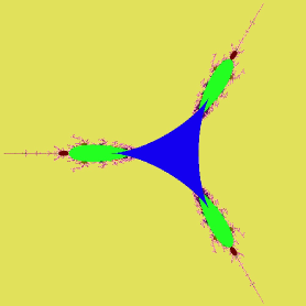
The multicorn of degree is defined as is connected. The multicorn of degree is called the tricorn.
It follows from classical works of Bowen and Ruelle [23, 30] that the Hausdorff dimension of the Julia set depends real-analytically on the parameter within every hyperbolic component of . Ruelle’s proof makes essential use of the fact that hyperbolic rational maps are expanding (this allows one to use the powerful machinery of thermodynamic formalism), and the Julia sets of hyperbolic rational maps move holomorphically inside every hyperbolic component.
The boundary of every hyperbolic component of odd period of is a simple closed curve consisting of exactly double parabolic parameters (also called ‘cusp points’) as well as parabolic arcs, each connecting two double parabolics. Moreover, any two parameters on a given parabolic arc have quasiconformally conjugate dynamics [18]. Since parabolic maps have a certain weak expansion property, and since there are real-analytic arcs of quasiconformally conjugate parabolic parameters on the boundary of every hyperbolic component of odd period of , it is natural to ask whether the Hausdorff dimension of the Julia set depends real-analytically on the parameter along these parabolic arcs.
However, an apparent obstruction to proving real-analyticity of Hausdorff dimension of the Julia set along the parabolic arcs is that the parabolic arcs are real one-dimensional curves, and hence one cannot find a holomorphic motion of the Julia sets (of the parabolic parameters) within the family of unicritical antiholomorphic polynomials. We circumvent this problem by constructing a strictly larger quasiconformal deformation class of the odd period simple parabolic parameters (also called ‘non-cusp’ parabolic parameters) of the multicorns so that the deformation is no longer contained in the family of unicritical antiholomorphic polynomials, but lives in a bigger family of holomorphic polynomials. This helps us to embed the parabolic arcs (which are real one-dimensional curves) in a complex one-dimensional family of quasiconformally conjugate parabolic maps. This proves the existence of holomorphic motion of the Julia sets under consideration (better yet, this proves structural stability of the odd period non-cusp parabolic maps along a suitable algebraic curve). This is performed in Section 3 by varying the critical Ecalle height over a bi-infinite strip by a quasiconformal deformation argument.
Having the complexification of the parabolic arcs (i.e. complex analytic parameter dependence of the persistently parabolic maps) at our disposal, we can apply results on real-analyticity of Hausdorff dimension of Julia sets of analytic families of meromorphic functions, as developed in [25], to our setting. The following theorem, which is proved in Section 4, can be naturally thought of as a version of Ruelle’s theorem on the boundaries of hyperbolic components:
Theorem 1.2 (Real-analyticity of HD Along Parabolic Arcs).
Let be a parabolic arc of and let be its critical Ecalle height parametrization. Then the function
is real-analytic.
It will transpire from the course of the proof that in good situations, the real-analyticity of Hausdorff dimension holds more generally on certain regions of the parabolic curves (see [16] for the definition of the curves) of various other families of polynomials.
As a by-product of the quasiconformal deformation step, we prove that the Ecalle height parametrization of the parabolic arcs of the multicorns is non-singular at all but possibly finitely many points.
Theorem 1.3.
Let be a parabolic arc of odd period of and be its critical Ecalle height parametrization. Then, there exists a holomorphic map such that:
-
(1)
The map agrees with the map on .
-
(2)
For all but possibly finitely many , .
In particular, the critical Ecalle height parametrization of any parabolic arc of has a non-vanishing derivative at all but possibly finitely many points.
In Section 5, we look at the curves in biquadratic polynomials, and prove that each cusp point (odd period double parabolic parameter) is a singular point (with at least a double tangent) of . In Section 6, we look at some more examples of the algebraic sets (in various families of polynomials), and try to understand the nature of their singularities as well the ‘dynamical’ behavior of these singular parameters. We do not prove any precise theorem here, we rather investigate some concrete examples, and give heuristic explanations of singularity/non-singularity, with a view towards a more general understanding of the topology of these algebraic sets.
This paper is a continuation of the author’s investigation of the parameter spaces of unicritical antiholomorphic polynomials [24, 18, 10]. These parameter spaces have played an important role in the recent work by various people [2, 3, 4, 5]. Therefore, notwithstanding the fact that the results of this paper are likely to hold in more general settings, it is worthwhile to record the ideas in the concrete case of unicritical antiholomorphic polynomials. It is worth mentioning that the present paper adds one more item to the list of topological differences between the multicorns and their holomorphic counterparts, the multibrot sets (these are the connectedness loci of unicritical holomorphic polynomials ). Clearly, the parameter dependence of the Hausdorff dimension of the Julia sets is far from regular on the boundary of the Mandelbrot set. It has been recently proved [8] that the multicorns are not locally connected, while the local connectivity of the Mandelbrot set is one of of the most prominent conjectures in one dimensional complex dynamics. In a recent work [10], we proved that rational parameter rays at odd-periodic angles of the multicorns do not land, rather they accumulate on arcs of positive length in the parameter space. This is in stark contrast with the fact that every rational parameter ray of the multibrot sets lands at a unique parameter. In [10], we also showed that the centers of the hyperbolic components, and the Misiurewicz parameters do not accumulate on the entire boundary of the multicorns. More such topological differences between the multibrot sets and the multicorns, including bifurcation along arcs, existence of real-analytic arcs of quasi-conformally equivalent parabolic parameters, discontinuity of landing points of dynamical rays, etc. can be found in [18].
2. Antiholomorphic Fatou Coordinates, Equators and Ecalle heights
In this section, we recall some basic facts about the parameter spaces of unicritical antiholomorphic polynomials. One of the major differences between the multicorns and the multibrot sets (which are the connectedness loci of unicritical holomorphic polynomials ) is that the boundaries of odd period hyperbolic components of the multicorns consist only of parabolic parameters.
Lemma 2.1 (Indifferent Dynamics of Odd Period).
The boundary of every hyperbolic component of odd period of consists entirely of parameters having a parabolic cycle of exact period . In appropriate local conformal coordinates, the -th iterate of such a map has the form with .
Proof.
See [18, Lemma 2.8]. ∎
This leads to the following classification of odd periodic parabolic points.
Definition 2.2 (Parabolic Cusps).
A parameter will be called a cusp point if it has a parabolic periodic point of odd period such that in the previous lemma. Otherwise, it is called a simple (or non-cusp) parabolic parameter.
In holomorphic dynamics, the local dynamics in attracting petals of parabolic periodic points is well-understood: there is a local coordinate which conjugates the first-return dynamics to the form in a right half place [15, Section 10]. Such a coordinate is called a Fatou coordinate. Thus the quotient of the petal by the dynamics is isomorphic to a bi-infinite cylinder, called an Ecalle cylinder. Note that Fatou coordinates are uniquely determined up to addition by a complex constant.
In antiholomorphic dynamics, the situation is at the same time restricted and richer. Indifferent dynamics of odd period is always parabolic because for an indifferent periodic point of odd period , the -th iterate is holomorphic with positive real multiplier, hence parabolic as described above. On the other hand, additional structure is given by the antiholomorphic intermediate iterate.
Lemma 2.3.
Suppose is a parabolic periodic point of odd period of with only one petal (i.e. is not a cusp) and is a periodic Fatou component with . Then there is an open subset with and so that for every , there is an with . Moreover, there is a univalent map with , and contains a right half plane. This map is unique up to horizontal translation.
Proof.
See [8, Lemma 2.3]. ∎
The map will be called an antiholomorphic Fatou coordinate for the petal . The antiholomorphic iterate interchanges both ends of the Ecalle cylinder, so it must fix one horizontal line around this cylinder (the equator). The change of coordinate has been so chosen that it maps the equator to the the real axis. We will call the vertical Fatou coordinate the Ecalle height. Its origin is the equator. The existence of this distinguished real line, or equivalently an intrinsic meaning to Ecalle height, is specific to antiholomorphic maps.
The Ecalle height of the critical value of is called the critical Ecalle height of , and it plays a special role in antiholomorphic dynamics. The next theorem proves the existence of real-analytic arcs of non-cusp parabolic parameters on the boundaries of odd period hyperbolic components of the multicorns.
Theorem 2.4 (Parabolic arcs).
Let be a parameter such that has a parabolic cycle of odd period, and suppose that is not a cusp. Then is on a parabolic arc in the following sense: there exists an injective real-analytic map such that for all , is a non-cusp parabolic parameter, the critical Ecalle height of is , the antiholomorphic polynomials have quasiconformally equivalent but conformally distinct dynamics, and is an interior point of the simple real-analytic arc .
Proof.
See [18, Theorem 3.2]. ∎
The simple real-analytic arc constructed in the above theorem is called a parabolic arc, and is denoted by . The parametrization of the parabolic arc given in the previous theorem is called the critical Ecalle height parametrization of .
The structure of the hyperbolic components of odd period plays an important role in the global topology of the parameter spaces.
Theorem 2.5 (Boundaries Of Odd Period Hyperbolic Components).
The boundary of every hyperbolic component of odd period of is a simple closed curve consisting of exactly parabolic cusp points as well as parabolic arcs, each connecting two parabolic cusps.
Proof.
See [18, Theorem 1.2]. ∎
3. Constructing an Analytic Family of Q.C. Deformations
Throughout this section, we fix a parabolic arc such that for each , has a -periodic parabolic cycle. Recall that there is a dynamically defined parametrization of , which is its critical Ecalle height parametrization . We will show that the polynomials on can be quasi-conformally deformed to yield an analytic family of q.c. conjugate maps; in particular, they will be structurally stable on a suitable algebraic curve.
We embed our family in the family of holomorphic polynomials . Since , the connectedness locus of this family intersects the slice in .
It will be useful to have the following characterization of the elements of amongst all monic centered polynomials of degree .
Lemma 3.1.
Let be a monic centered polynomial of degree . Then the following are equivalent:
-
(1)
with .
-
(2)
has exactly distinct critical points with for each and such that .
Proof.
The critical points of any are and the roots of the equation . Since , these points are all distinct and has local degree at each of them. The other property is immediate.
Let, . Since each () maps in a -to- fashion to and the degree of is , these must be all the pre-images of . Therefore, , where (here, we have used the fact that is monic). Note that the critical points of are precisely the zeroes and the critical points of . Since we have used up the distinct zeroes of and are left with only one critical point of , it follows that this critical point must be the only critical point of . Hence, must be unicritical. A brief computation (using the fact that is centered) now shows that , for some . The fact that all the are distinct tells that must be non-zero. Thus, we have shown that with , . ∎
Remark 1.
Condition (2) of the previous lemma is preserved under topological conjugacies.
Before we can turn our attention to the algebraic curves that are the principal objects of study of this paper, we need to take a brief digression to algebra. In what follows, we will discuss the properties of discriminants and resultants of complex polynomials.
For a monic complex polynomial with roots , the discriminant of is defined as:
It is evident from the definition of the discriminant that has a multiple (or repeated) root if and only if vanishes. Moreover, is a symmetric function of the roots of , hence it can be expressed as a polynomial function of the elementary symmetric functions in the variables . But the elementary symmetric functions in , up to sign, coincide with the coefficients of . Therefore, can be written as a polynomial in the coefficients of (compare [7, §14.6]).
In a similar vein, the resultant of two univariate polynomials and is a polynomial in the coefficients of and which vanishes if and only if and have a common root; i.e. if and only if . It is sometimes desirable to generalize the notion of resultants to be able to predict the exact degree of the gcd of and in terms of their coefficients. This can be done by the so-called subresultants, which are polynomials in the coefficients of and , and whose order of vanishing tells us the degree of the gcd of the two polynomials and . We refer the readers to [BPC, §4.2.2] for the precise definition of subresultants.
The main property of subresultants that will be used in this paper is the following.
Lemma 3.2.
For two univariate polynomials and over a domain (of degree and respectively, such that ), for some if and only if , where each is a polynomial expression in the coefficients of and .
Proof.
See [BPC, Proposition 4.25]. ∎
We will now use the concept of discriminants to define parabolic curves in the parameter space of the family . Since every antiholomorphic polynomial on a parabolic arc has a parabolic cycle of odd period and multiplier , its holomorphic second iterate also has a -periodic parabolic cycle of multiplier (note that as is odd, we have that and are relatively prime). Therefore, under the embedding of the family of unicritical antiholomorphic polynomials into the family of holomorphic polynomials , the image of the parabolic arc sits in the set of all -periodic parabolic parameters of multiplier . However, if has a -periodic parabolic cycle of multiplier , then has a multiple root. Therefore by definition of discriminants, the parabolic arc embeds into the set:
.
Note that ; i.e. it is a polynomial in the variable with coefficients from the ring . It now follows from our discussion on discriminants that is a polynomial in the variables , with complex coefficients. Hence is an algebraic curve in .
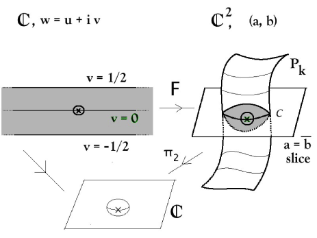
We are now in a position to prove the main technical lemma, which allows us to embed the parabolic arc in a complex one-dimensional deformation space contained in . The idea of the proof is as follows. For any , the second iterate of the antiholomorphic polynomial is a holomorphic polynomial with two infinite critical orbits. Both these critical orbits are attracted by the unique parabolic cycle of , and hence we can choose two representatives of these two critical orbits in a fundamental domain of an attracting petal of . The difference of the attracting Fatou coordinates of these two chosen representatives (the difference does not depend on the choice of the representatives as long as they are chosen from the same fundamental domain) turn out to be a conformal conjugacy invariant of the polynomial. This invariant will be called the Fatou vector of the polynomial. We will deform the polynomial in such a way that the qualitative behavior of the dynamics remains the same, but the Fatou vector varies over a bi-infinite strip. Thus, each deformation would give us a topologically conjugate, but conformally different polynomial.
Lemma 3.3 (Extending the Deformation).
Let . There exists an injective holomorphic map
,
with such that for any , where is the critical Ecalle height parametrization of the parabolic arc. Further, all the polynomials have q.c.-conjugate (but not conformally conjugate) dynamics.
Proof.
We construct a larger class of deformations which strictly contains the deformations constructed in [18, Theorem 3.2]. Choose the attracting Fatou coordinate (at the parabolic point on the boundary of the unique Fatou component of that contains ) such that the unique geodesic invariant under the antiholomorphic dynamics maps to the real line and the critical value has Ecalle coordinates (this is possible since ). The polynomial has two critical values and . The map sends to the Fatou component containing . The Ecalle coordinates of is . We will simultaneously change the Ecalle coordinates of and in a controlled way, so that each perturbation gives a conformally different polynomial.
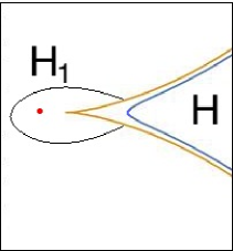
Setting , we can change the conformal structure within the Ecalle cylinder by the quasi-conformal homeomorphism of (compare Figure 2):
for
Translating the map by positive integers, we get a q.c. homeomorphism of a right-half plane that commutes with the translation . By the coordinate change , we can transport this Beltrami form (defined by this quasiconformal homeomorphism) into all the attracting petals, and it is forward invariant under . It is easy to make it backward invariant by pulling it back along the dynamics. Extending it by the zero Beltrami form outside of the entire parabolic basin, we obtain an -invariant Beltrami form. Using the Measurable Riemann Mapping Theorem with parameters, we obtain a qc-map integrating this Beltrami form. Furthermore, if we normalize such that the conjugated map is always a monic and centered polynomial, then the coefficients of this newly obtained polynomial will depend holomorphically on (since the Beltrami form depends complex analytically on ).
We need to check that this new polynomial belongs to our family . But this readily follows from Lemma 3.1 and the remark thereafter. Therefore, this new polynomial must be of the form . Since the coefficients of depend holomorphically on , the maps and are holomorphic. Its Fatou coordinate is given by . Note that the Ecalle coordinates of the two representatives of the two critical orbits of are and .
Thus, we obtain a complex analytic map (compare Figure 3). For real values of , the map commutes with the map , and hence, the corresponding Beltrami form is invariant under the antiholomorphic polynomial (recall that conjugates to in the attracting petal). Therefore, is again a unicritical antiholomorphic polynomial in the family . In particular, for , the critical Ecalle height of is . Therefore,
By construction, all the are quasiconformally conjugate to , and hence to each other. We now show that they are all conformally distinct. Define the Fatou vector of to be the quantity , where is the Fatou coordinate of . Since the Fatou coordinate is unique up to addition by a complex constant, the Fatou vector defined above is a conformal conjugacy invariant. The Fatou vector of is given by , which is different for different values of . Hence, the polynomials are conformally nonequivalent. In particular, the map is injective.
It remains to show that for any , . It is easy to see that each has a parabolic cycle of exact period (both critical orbits are contained in the Fatou set and converge to a -periodic orbit sitting on the Julia set). Also, the first return map leaves the unique petal attached to every parabolic point invariant; so the multiplier of the parabolic cycle must be . Hence, . ∎
Remark 2.
It was possible to construct this larger class of deformation since we worked with the polynomial viewing it as a member of the family . Working in the family of unicritical antiholomorphic polynomials would have only allowed us to construct the real one-dimensional parabolic arcs, as was done in [18, Theorem 3.2]. Indeed, the Beltrami form constructed in the previous lemma is invariant under for all , but it is invariant under only when is real. This is because we obtained the quasiconformal deformations via the map , which commutes with only when .
Remark 3.
Various dynamically defined quantities, e.g. the fixed point index, the Ecalle-Voronin coefficients of the parabolic cycle of depend holomorphically on .
Recall that the set of singular points of an algebraic curve (where is a complex polynomial in two variables and ) is defined as
It is worth mentioning that (by the implicit function theorem) an algebraic curve is locally a manifold near its non-singular points. It is a well-known fact that an affine algebraic curve has at most finitely many singular points.
Proof of Theorem 1.3.
Part (i) follows from Lemma 3.3. The required map is given by .
We will show that if is a non-singular point of the algebraic curve , then the map has a non-vanishing derivative at . Since any affine algebraic curve has at most finitely many singular points, this will complete the proof of the theorem.
By the definition of non-singularity, one of the partial derivatives or is non-zero at . Let Then there exists and a holomorphic map such that and for some if and only if . Therefore, the projection map is an injective holomorphic map on an open neighborhood (in the subspace topology) of . It follows from Lemma 3.3 that the map is an injective holomorphic map on an open neighborhood . Hence, it has a non-vanishing derivative at , i.e. .
Writing and , we see that
It follows that , i.e. . ∎
Remark 4.
One can easily compute that the algebraic curve of the family is non-singular at each point of the parabolic arcs of period of the tricorn. Hence, the critical Ecalle height parametrization is indeed non-singular for the period parabolic arcs of the tricorn. However, we conjecture that the critical Ecalle height parametrization of any parabolic arc of is non-singular everywhere.
4. Real-Analyticity of Hausdorff Dimension
In this section, we prove real-analyticity of Hausdorff dimension of the Julia sets along the parabolic arcs by applying certain real-analyticity results from [25] to holomorphic family of parabolic maps constructed in the previous section.
Real-analyticity of Hausdorff dimension of Julia sets of hyperbolic maps is well-known due to the work of Ruelle and Bowen on thermodynamic formalism [23, 30]. The classical theory of thermodynamic formalism was developed (or at least works best) primarily for expanding maps. Since such maps admit Markov partitions, their dynamical properties can be conveniently studied by looking at the associated sub-shifts of finite type. In this setting, the largest eigenvalue of the so-called Ruelle operator is intimately connected with the Hausdorff dimension of the limit set. Moreover, a crucial spectral gap property of the largest eigenvalue and the fact that expanding maps are structurally stable (i.e. the qualitative behavior of the dynamics remains stable under small perturbations) help one show that Hausdorff dimension is a real-analytic function of the parameter.
Recall that a rational map is called parabolic if it has at least one parabolic cycle and every critical point of the map lies in the Fatou set (i.e. is attracted to an attracting or a parabolic cycle). Parabolic maps have a certain weak expansion property that makes it possible to use tools from thermodynamic formalism to investigate the finer fractal properties of their Julia sets. However, in the absence of Markov partitions, such a study requires much heavier machinery. We do not want to delve deep into this topic here, rather we would limit ourselves to describing how the main theorem of [25] applies to our context, as well as pointing out the salient differences between the hyperbolic and parabolic setting.
The following concept of radial Julia sets was introduced by Urbański and McMullen [26, 14], and its importance stems from the fact that the dynamics at the radial points of a Julia set have a strong expansion property.
Definition 4.1 (Radial Julia Set).
A point is called a radial point if there exists and an infinite sequence of positive integers such that there exists a univalent inverse branch of defined on sending to for all . The set of all radial points of is called the radial Julia set and is denoted as . Equivalently, the radial Julia set can be defined as the set of points in whose -limit set non-trivially intersects the complement of the post-critical closure.
For a radial point , there exists a sequence of iterates accumulating at a point outside the post-critical closure and hence, there exists a sequence of univalent inverse branches of defined on some sending to for all . Such a sequence necessarily forms a normal family and any limit function must be a constant map (compare [1, Theorem 9.2.1, Lemma 9.2.2]). This shows that the sequence of univalent inverse branches of are eventually contracting; in other words, .
For parabolic rational maps, one has a rather simple but useful description of the radial Julia set. The following proposition was proved in [6], we include the proof largely for the sake of completeness.
Lemma 4.2.
Let be a parabolic rational map and let be the set of all parabolic periodic points of . Then, . In particular, .
Proof.
For a parabolic rational map, the post-critical closure intersects the Julia set precisely in , which is a finite set consisting of (parabolic) periodic points. Starting with any point of , one eventually lands on under the dynamics and the existence of infinitely many post-critical points in every neighborhood of obstructs the existence of infinitely many univalent inverse branches. It follows that .
It remains to prove the reverse inclusion. By passing to an iterate, one can assume that . By the description of the local dynamics near a parabolic point [15, §10], there is a neighborhood of the parabolic points that is contained in the union of the attracting and repelling petals. By continuity, there exists a such that for and . We claim that for any , there exists a sequence of positive integers such that the sequence lies outside . Otherwise, there would exist an such that . Then, there exists some such that . But since each belongs to the repelling petal, it follows that , a contradiction to the assumption that . Finally, observe that any point in has a small neighborhood disjoint from the post-critical set. Since is a compact metric space, there exists a such that the neighborhood of any point of is disjoint from the post-critical set. Therefore, the balls are disjoint from the post-critical closure and hence, there exists a univalent inverse branch of defined on sending to for all . This proves that .
The final assertion directly follows as the set is countable. ∎
We should emphasize that so far as Hausdorff dimension is concerned, the previous lemma guarantees that we do not lose anything by restricting our attention to the radial Julia set.
Conformal measures have played a crucial role in the study of the dimension-theoretic properties of rational maps. It is worth mentioning in this regard that conformal measures satisfy a weak form of Ahlfors-regularity at the radial points of a Julia set. More precisely, by an immediate application of Koebe’s distortion theorem and the expansion property at the radial points discussed above, one obtains that for every point in , there exists a sequence of radii converging to () such that if is a -conformal measure for , then
for some constant depending on and .
Before we state the main technical theorem from [25], we need a couple of more definitions and facts from thermodynamic formalism. We will assume familiarity with the basic definitions and properties of topological pressure [27], [28, §9]. The behavior of the pressure function (where is the topological pressure) has been extensively studied by many people in the context of rational and transcendental maps. For hyperbolic rational maps, the pressure function is strictly decreasing and vanishes at a unique real number. The following result discusses the corresponding situation for parabolic maps.
Theorem 4.3.
[6] For a parabolic rational map ,
-
(1)
The function is continuous, non-increasing and non-negative.
-
(2)
such that,
-
(a)
for ,
-
(b)
for ,
-
(c)
is injective.
-
(a)
The Hausdorff dimension of the Julia set of a hyperbolic map is equal to the unique zero of the associated pressure function. The next theorem relates the Hausdorff dimension of the Julia set to the the minimal zero of the pressure function and the minimum exponent of -conformal measures for parabolic rational maps.
Theorem 4.4.
[6] For a parabolic rational map , the following holds:
A more elaborate account of these lines of ideas can be found in the expository article of Urbański [6, 26].
Definition 4.5.
A meromorphic function is called tame if its post-singular set does not contain its Julia set.
Clearly, parabolic polynomials are tame. For tame rational maps, there exist nice sets [13, 21] giving rise to conformal iterated function systems with the property that the Hausdorff dimension of the radial Julia set is equal to the common value of the Hausdorff dimensions of the limit sets of all the iterated function systems induced by all nice sets (compare [25, §2,3]). One can define the pressure function for these iterated function systems (induced by the nice sets) and the system is called strongly -regular if there is such that and if there is such that . The fact that the conformal iterated function systems arising from parabolic rational maps satisfy this property, can be proved as in Theorem 4.3.
We are now prepared to state the main result from [25] which is at the technical heart of our real-analyticity result.
Theorem 4.6.
[25, Theorem 1.1] Assume that a tame meromorphic function is strongly - regular. Let be an open set and let be an analytic family of meromorphic functions such that
-
(1)
for some ,
-
(2)
there exists a holomorphic motion such that each map is a topological conjugacy between and on .
Then the map is real-analytic on some neighborhood of .
Proof of Theorem 1.2.
Let be a parabolic arc and be its critical Ecalle height parametrization. It follows from Lemma 3.3 that there exists an injective holomorphic map and an analytic family of q.c. maps with . Setting , and , we see that all the conditions of Theorem 4.6 are satisfied and hence, the function is real-analytic. Restricting the map to the reals, we conclude that the map is real-analytic. The result now follows from Lemma 4.2. ∎
Remark 5.
Parabolic curves arise naturally in the study of the parameter spaces of higher degree polynomials and the techniques used in this article can be generalized to prove corresponding statements about the real-analyticity of Hausdorff dimension of the Julia sets on these curves, under suitable conditions. In particular, the real-analyticity of continues to hold on regions of parameter spaces where the maps only have attracting or parabolic cycles and such that all the critical points converge to these cycles.
The parabolic arcs of the multicorns inherit the real-analyticity property from the connectedness loci of the sub-family of all polynomials of degree .
5. of Biquadratic Polynomials
We observed that the parabolic arcs of period of are naturally embedded in the algebraic curve . Moreover, for any on a parabolic arc of period , the polynomial is structurally stable along the curve .
The curve is customarily referred to as [16] (since the corresponding maps have a -periodic orbit of multiplier ). The topology of these curves plays an important role in the understanding of the parameter spaces of the maps under consideration. In order to analyze the types of singularities of and their dynamical meaning, we shall have need for some general notions about singularities of holomorphic function germs.
5.1. Degenerate Singularities, Morsification, and Milnor Number
A holomorphic function germ is said to be singular at a point if the first order partial derivatives are all zero at . In this subsection, we will only be concerned with isolated singularities; i.e. those singular points that have a small neighborhood such that is the only singular point of in . We say that a point is a degenerate singular point of if is a singular point and the Hessian matrix of all second order partial derivatives has zero determinant at ; i.e.
Otherwise, the singularity is called non-degenerate. Note that non-degenerate singularities are the simplest kind of singularities where the analytic set germ given by the vanishing of locally looks like the transverse intersection of two non-singular branches. In other words, the analytic set has two distinct tangent planes at a non-degenerate singularity. It is therefore desirable to think of a degenerate singularity of as the merger of several non-degenerate singularities. Intuitively, if one perturbs suitably, then an isolated degenerate singularity of splits up into a number of non-degenerate isolated singularities. This number, which we will formally define below, measures the complexity of a singularity.
Definition 5.1 (Morsification).
A -parameter family of deformations of a holomorphic function germ with an isolated singularity is called a morsification if for (small) all singularities of are non-degenerate.
Any function with an isolated singularity admits a morsification (compare [29, Proposition 6.5.4]. This leads to the following definition of the Milnor number.
Definition 5.2 (Milnor Number).
Let be a morsification of , which has an isolated singularity at . Then for small , the total number of non-degenerate singularities of near is called the Milnor number of at (the isolated singularity) . It is denoted by .
Equivalently, one can define the Milnor number algebraically as follows. Let be the ring of holomorphic function germs , and be the Jacobian ideal of :
The local algebra of is then given by:
The Milnor number is then equal to the dimension of as a complex vector space:
It may be instructive to compute the Milnor number of a couple of simple functions germs using the algebraic description.
Example 1). The function has a singularity at with non-vanishing Hessian. Since , and , the Jacobian ideal is . Hence its local algebra is given by , which has dimension . Therefore, the Milnor number is . In fact, any function germ with a non-degenerate singularity has Milnor number .
Example 2). The function has a singularity at with vanishing Hessian. Since , and , the Jacobian ideal is . Hence its local algebra is given by , which has dimension . Therefore, the Milnor number is . It is not hard to see that under small perturbations, the degenerate singularity of splits into two distinct non-degenerate singularities.
5.2. Dynamically Defined Morsifications
With these general tools at our disposal, we now return to the study of the singularities of the curves .
For and , the curve of the family of polynomials has a very simple description. One easily computes that
The set of singular points of is , , , , , where is a primitive third root of unity. Note that these points correspond precisely to the cusps at the ends of the parabolic arcs of period of the tricorn. In fact, a simple calculation shows that
.
The same is true for the other singular points. In particular, each singular point of is an ordinary cusp point (i.e. a cusp of the form at ). By the classical degree-genus formula for singular curves (compare [12, Theorem 7.37]), it follows that the genus of is . Hence, after desingularization (and compactification), of the family is the Riemann sphere .
It will be useful to consider a family of dynamically defined deformations of the function above so that the perturbed functions only have non-singular singularities. To be precise, we will look at the curve , which consists of parameters such that has a fixed point of multiplier . In other words, lies on if the polynomials and have a common root. This allows us to define the algebraic curve in terms of (sub-)resultants as
Let us discuss the singularities of (with , sufficiently small) near . Each has two non-degenerate critical points close to . Hence, the deformation provides a morsification of the degenerate singularity of (compare Figure 4). Observe that this is in consonance with the fact that is a degenerate singularity of with Milnor number .
One of these two critical points of lies on . In fact, belongs to a period hyperbolic component (bifurcating from the principal hyperbolic component at ) of . Therefore, , and its Milnor number is . One can dynamically explain the existence of the singular point of as follows: the map has two distinct fixed points of multiplier , and hence is a point of transverse intersection of two smooth local branches (each defined by the condition that has a fixed point of multiplier ) of .
Using these information on the family , we will now show that the cusp points of period (recall Definition 2.2), lying on the boundaries of hyperbolic components of odd period of the tricorn, are singular points (with at least a double tangent) of of the family .
Proposition 1.
Let be a parabolic arc of odd period of , and be a double parabolic point (cusp point) at the end of . Then is a singular point (with at least a double tangent) of of .
Proof.
Recall that the set of singular points of is , , , , (where is a primitive third root of unity), and these are precisely the cusp points of period . We will denote the principal hyperbolic component of the family by , and the hyperbolic component (of ) of period that bifurcates from at the parameter by .
Let be the hyperbolic component of period of with , and be the hyperbolic component of period of that bifurcates from at . We again consider the -parameter family of deformations (the curve of parameters with an -periodic cycle of multiplier ) of . More precisely, we define , where is the square-free part of .
By [9, Theorem C], the straightening map induces biholomorphisms and , and (this is no loss of generality as one of the maps , or satisfies this property). Since , sends a polynomial with an attracting -cycle of multiplier to a polynomial with an attracting fixed point of multiplier ; i.e. . Therefore,
Clearly, lies on the curve ; i.e. . We claim that is a non-degenerate critical point of , for each . Recall that as , hence as (by [11, Theorem 6.3], the straightening map extends as a homeomorphism from the closure of onto the closure of ). Since (for small enough) is an arbitrarily small perturbation of , this claim implies that any small perturbation of has at least one non-degenerate critical point near . Hence, by definition, the Milnor number is at least (compare [29, Lemma 6.5.5]); i.e. is a singular point of .
We will now prove the claim that is a non-degenerate critical point of ; i.e. it has Milnor number . Note that since () is a non-degenerate critical point of and is a biholomorphism from onto , it follows (by a simple computation using chain rule) that () is a non-degenerate critical point of . Therefore, the Milnor number . It now suffices to look at the relation between and locally near . This is a routine exercise in analytic geometry, we work out the details for the sake of completeness. Consider the ring of germs of holomorphic functions (in two variables) defined in some neighborhood of . Since and are both square-free as elements of and their vanishing define the same analytic set germ near (namely the germ of at ), it follows that there exists an invertible element such that as elements of . But then, their Milnor numbers are equal; i.e. .
To conclude the proof, we need to justify that has a double tangent at . A direct computation shows that the two distinct tangent lines of at tend to coincide as tends to (in fact, they both tend to , which is a double tangent of at ). This property is preserved by the biholomorphism . Hence the two distinct tangent lines of at tend to coincide as tends to , and they form a double tangent line of at . ∎
On the other hand, we observed that the curve is non-singular everywhere along the parabolic arcs of period ; i.e. . Consequently, for , the dynamically defined deformations have no critical points near . Since this property is preserved under the straightening map , and since the curve germs form a -parameter family of deformations of , we have the following proposition:
Proposition 2.
Let be a parabolic arc of odd period of , and be its critical Ecalle height parametrization. Then for each , is a non-singular point of . In particular, the critical Ecalle height parametrization of has a non-vanishing derivative at all points; i.e. for every .
6. Singularities of : Some Examples
In this section, we will take a closer look at the algebraic sets that appeared earlier in the article. The singular locus of these algebraic sets are important in understanding their topology. Indeed, the local topology of a curve near a singular point is completely determined by its equisingularity class. In particular, one can associate a link with a plane curve singularity such that two equisingular curves have isotopic links, and the curve is locally homeomorphic to the cone on [29, Theorem 5.5.9, Lemma 5.2.1]
Definition 6.1.
Let be a holomorphic family of holomorphic polynomials of degree , depending algebraically on parameters . The algebraic set is defined as the set of parameters in such that has a parabolic cycle of period and multiplier . In algebraic terms,
,
Observe that our definition does not ensure that for every , the corresponding polynomial has a periodic orbit of exact period with multiplier . Indeed, our definition allows to contain all parameters such that the corresponding polynomials possess a -periodic orbit (where ) with multiplier a -th root of unity. However, parameters having a -periodic orbit (where ) with multiplier a -th root of unity determine a polynomial that divides , and one can factor them out from to obtain an algebraic curve consisting precisely of those maps with an -cycle with multiplier . However, we assure the readers that this ambiguity in defining will not be of importance to us since we will mostly be interested in local properties (e.g. singularity) that are not affected by the additional components of .
In what follows, we will look at some more examples of (in various families of polynomials), and will try to understand the nature of their singularities as well as the ‘dynamical’ behavior of these singular parameters. It is not our aim to prove any precise theorem here, we only intend to investigate some natural examples and to give heuristic explanations of the phenomena, which should pave the way for a more general understanding of the topology of these algebraic sets.
1. We first consider families such that , a generic has two infinite critical orbits, and is a complex curve. For any , we can write in appropriate local coordinates in a neighborhood of a parabolic periodic point as . Such a parabolic point has petals and each petal attracts at least one infinite critical orbit. Since every map in our family has at most infinite critical orbits, it follows that . Furthermore, any has at most two disjoint parabolic cycles (since there are at most two infinite critical orbits). We, therefore, have to consider the following three cases.
(a) (Unique parabolic cycle with : non-singular point). Let be a sufficiently small neighborhood of in . The double root of splits into two simple roots in . On a double cover over , ramified only over , we can follow these two simple periodic points holomorphically as functions and . In , corresponds to the smooth (complex -dimensional) analytic set (some care is needed here; if are the local coordinates on , one needs to show that the map is a local biholomorphism). This suggests that is a non-singular point of .
Alternatively, in a sufficiently small neighborhood of in , we have , where are holomorphic in , and is non-vanishing. Hence, . In a generic situation, can be taken as local coordinates on , and locally near , will look like at . Hence, would be a non-singular point of .
(b) (Unique parabolic cycle with : ordinary cusp). Let be a sufficiently small neighborhood of in . The triple root of splits into three simple roots in . On a triple cover over , ramified only over , we can follow these three simple periodic points holomorphically as functions , and . In , corresponds to the complex -dimensional analytic set , and the parameter corresponds to . This analytic set is not regular at : two of the three conditions determine the same curve, and hence, the analytic set has two coincident tangent lines (or a tangent line of multiplicity ) at . This suggests that is an ordinary cusp singularity of .
Alternatively, in a sufficiently small neighborhood of in , we have , where are holomorphic in , and is non-vanishing. Hence, . In a generic situation, can be taken as local coordinates on , and will have a singularity of the form at .
(c) (Two parabolic cycles each with : ordinary double point). Let be a sufficiently small neighborhood of in . Then has two (distinct) double roots. When is perturbed in , these two double roots split into two pairs of simple roots. On a double cover over , ramified only over , we can follow these two pairs of simple periodic points as two pairs of holomorphic functions and . In , corresponds to the complex -dimensional analytic set , and the parameter corresponds to the point of self-intersection . In other words, corresponds to the union of two (different) branches given by and , and corresponds to the point where these two branches intersect (transversally). Therefore, is an ordinary double point (with non-vanishing Hessian and two distinct tangent lines) of .
Examples. i) In Subsection 5, we discussed the properties of of the family : the only singularities of this algebraic curve correspond to the parameters with double parabolic points, and each of these singularities is of the form at . Every other point of this curve is non-singular.
ii) Let us look at the family of monic centered cubic polynomials . For this family, we have
Once again, the only singular point of this curve is , which is the only double parabolic point of . In fact, is a double point of with vanishing Hessian. To better visualize this singularity, we may consider the following dynamically defined morsification. The algebraic curve consisting of all parameters for which has a fixed point of multiplier is referred to as . More precisely, for , we define
where of two polynomial and in one complex variable denotes the resultant of and .
Then is a morsification of in the sense that for , has two non-degenerate (i.e. with non-vanishing Hessian) critical points at and . Let us try to understand the formation of the cusp-type singularity of at in the following dynamical fashion. For , has two distinct fixed points of multiplier . Hence, is the point of intersection of two transversal branches of , and is a node-type singular point of (i.e. a double point with two distinct tangent lines). At the other critical point of , has two distinct fixed points of multiplier . As , these two critical points (each having Milnor number ) of coalesce to form the critical point (with Milnor number ) of , and all the fixed points coalesce to form a triple fixed point of .
iii) We now consider of the family . The parameter is a co-root of a hyperbolic component of period of . The polynomial has two simple parabolic fixed points, and is an ordinary double point (with non-vanishing Hessian and two distinct tangent lines) of of this family.
The local topology of near these singularities can be studied via the singularity link and the Milnor fibration (compare [17]). In fact, in the first two examples above, is locally (near the singularity) a cone over the trefoil knot. In the third example, is locally a cone over the Hopf link.
2. We now look at families with such that a generic has three infinite critical orbits. For simplicity, we will restrict ourselves to the case (this case is already more complicated than the case where ). As above, for any , we can write in appropriate local coordinates in a neighborhood of a parabolic point as with . For ease of exposition, let us work with the family of monic centered quartic polynomials. Then,
To take a closer look at the different types of singularities, we need to consider four sub-cases.
(a) (Unique parabolic fixed point with : non-singular point). The treatment of this case is similar to that of Case 1(a).
(b) (Unique parabolic fixed point with : triple point). The only parameter for which has a parabolic cycle with three petals is . A simple yet lengthy computation shows that is a singular point of ; in particular, it is a triple point with three coincident tangents (or a tangent of multiplicity ). A heuristic reasoning for this kind of singularity can be given along the same lines of Case 1(b).
(c) (Non-isolated singularities). Since is a two-dimensional algebraic set, it is perhaps not surprising that it has non-isolated singularities along a complex one-dimensional algebraic subset. These non-isolated singular parameters are given by the intersection of the algebraic sets
This is, in fact, the intersection of with . Each point of is a singular point of .
As is clear from the defining property, for each , the corresponding polynomials and have at least two common factors. The case where they have three common factors is already covered in the previous case, so we will now be concerned with the case . This can happen in two different ways.
i) (Two parabolic fixed points each with ). Each parameter of the form () belongs to , and the corresponding polynomial has two distinct simple parabolic fixed points . This case is similar to Case 1(c); the singularities are formed by the transversal intersection of two branches of the algebraic set. Hence, each () is a double point, and there are two tangents at each such singularity.
ii) (Unique parabolic fixed point with ). For each , has a unique parabolic fixed point with two petals. Each such parameter is a double point with a single tangent of multiplicity . A heuristic reasoning for this kind of singularity can be given along the same lines of Case 1(b).
Let us summarize our observations regarding the singular locus of of degree monic centered polynomials. The singular locus admits a natural stratification , where
Here, is a triple point of with a tangent of multiplicity , each point of is a double point with two distinct tangents, and each point of is a double point with a tangent of multiplicity . Therefore, the Milnor fibrations at any two points of have the same fibration type.
In general, we should ask the following questions, which are clearly motivated by the preceding analysis.
Question.
Let be a holomorphic family of holomorphic polynomials of degree , depending algebraically on parameters .
-
(1)
Does every singularity of occur either due to orbit mergers (giving rise to cusp-type singularities) or due to transverse intersection of more than one branches, each defining a periodic orbit of multiplier (giving rise to node-type singularities)?
-
(2)
Can we classify the types of singularities of in terms of dynamical properties of the singular parameters?
-
(3)
Study the topology of near its singularities, especially near the non-isolated ones.
References
- [1] A. F. Beardon, Iteration of Rational Functions, Complex Analytic Dynamical Systems Series: Graduate Texts in Mathematics, Vol. 132, Springer-Verlag, 1991.
- [2] A. Bonifant, X. Buff and J. Milnor, Antipode preserving cubic maps: the fjord theorem, arXiv: 1512.01850.
- [3] A. Bonifant, X. Buff and J. Milnor, Antipode preserving cubic maps II: tongues and the ring locus, work in progress.
- [BPC] S. Basu, R. Pollack and M.-F. Coste-Roy, Algorithms in Real Algebraic Geometry, 2nd edition, Springer, Berlin, 2006.
- [4] J. Canela, N. Fagella and A. Garijo, On a family of rational perturbations of the doubling map, Journal of Difference Equations and Applications, 21 (2015), 715–741.
- [5] W. Bergweiler and A. Eremenko, Green’s function and anti-holomorphic dynamics on a torus, Proc. Amer. Math. Soc., 144 (2016), 2911–2922.
- [6] M. Denker and M. Urbański, Hausdorff and conformal measures on Julia sets with a rationally indifferent periodic point, J. London Math. Soc., 43(2) (1991), 107–118.
- [7] D. S. Dummit and R. M. Foote, Abstract Algebra, 3rd Edition, John Wiley and Sons, Inc., 2003.
- [8] J. H. Hubbard and D. Schleicher, Multicorns are not path connected, in Frontiers in Complex Dynamics: In Celebration of John Milnor’s 80th Birthday (eds. A. Bonifant, M. Lyubich and S. Sutherland), Princeton University Press, (2014), 73–102.
- [9] H. Inou and J. Kiwi, Combinatorics and topology of straightening maps, I: compactness and bijectivity, Advances in Mathematics, 231 (2012), 2666–2733.
- [10] H. Inou and S. Mukherjee, Non-landing parameter rays of the multicorns, Inventiones Mathematicae, 204 (2016), 869–893.
- [11] H. Inou and S. Mukherjee, Discontinuity of straightening in antiholomorphic dynamics, arXiv: 1605.08061.
- [12] Frances Kirwan, Complex Algebraic Curves, Cambridge University Press, Cambridge, 1992.
- [13] J. Rivera-Letelier, A connecting lemma for rational maps satisfying a no-growth condition, Ergodic Theory and Dynamical Systems, 27(2) (2007), 595–636.
- [14] C. T. McMullen, Hausdorff dimension and conformal dynamics II: geometrically finite rational maps, Commentarii Mathematici Helvetici, 75(4) (2000), 535–593.
- [15] J. Milnor, Dynamics in one complex variable, 3rd Edition, Princeton University Press, New Jersey, 2006.
- [16] J. Milnor, Remarks on iterated cubic maps, Experiment. Math., 1(1) (1992), 5–24.
- [17] J. Milnor, Singular Points of Complex Hypersurfaces, Annals of Mathematics Studies. Princeton University Press, New Jersey, 1968.
- [18] S. Mukherjee, S. Nakane and D. Schleicher, On multicorns and unicorns II: bifurcations in spaces of antiholomorphic polynomials, Ergodic Theory and Dynamical Systems, 37 (2017), 859–899.
- [19] D. R. Mauldin and M. Urbański, Graph Directed Markov Systems: Geometry and Dynamics of Limit Sets, Cambridge University Press, Cambridge, 2003.
- [20] S. Nakane, Connectedness of the tricorn, Ergodic Theory and Dynamical Systems, 13 (1993), 349–356.
- [21] N. Dobbs, Nice sets and invariant densities in complex dynamics, Math. Proc. Cambridge Philos. Soc., 150(1) (2011), 157–165.
- [22] S. Nakane and D. Schleicher, On multicorns and unicorns I: antiholomorphic dynamics, hyperbolic components, and real cubic polynomials, International Journal of Bifurcation and Chaos, 13 (2003), 2825–2844.
- [23] D. Ruelle, Repellers for real analytic maps, Ergodic Theory and Dynamical Systems, 2(1) (1982), 99–107.
- [24] S. Mukherjee, Orbit portraits of unicritical antiholomorphic polynomials, Conformal Geometry and Dynamics of the AMS, 19 (2015), 35–50.
- [25] B. Skorulski and M. Urbański, Finer fractal geometry for analytic families of conformal dynamical systems, Dynamical Systems, 29 (2014), 369–398.
- [26] M. Urbański, Measures and dimensions in conformal dynamics, Bull. Amer. Math. Soc., 40 (2003), 281–321.
- [27] P. Walters, A variational principle for the pressure of continuous transformations, Amer. J. Math., 97 (1979), 937–971.
- [28] P. Walters, An introduction to ergodic theory, Graduate Texts in Mathematics, Volume 79, Springer, 1982.
- [29] C. T. C. Wall, Singular Points of Plane Curves, London Mathematical Society Student Texts (vol. 63), Cambridge University Press, 2004.
- [30] M. Zinsmeister, Thermodynamic Formalism and Holomorphic Dynamical Systems, SMF/AMS Texts and Monographs, Volume 2, 2000.