A multilevel correction method for optimal controls of elliptic equation

Abstract:    We propose in this paper a multilevel correction method to solve optimal control problems constrained by elliptic equations with the finite element method. In this scheme, solving optimization problem on the finest finite element space is transformed to a series of solutions of linear boundary value problems by the multigrid method on multilevel meshes and a series of solutions of optimization problems on the coarsest finite element space. Our proposed scheme, instead of solving a large scale optimization problem in the finest finite element space, solves only a series of linear boundary value problems and the optimization problems in a very low dimensional finite element space, and thus can improve the overall efficiency for the solution of optimal control problems governed by PDEs.

Keywords:    Optimal control problems, elliptic equation, control constraints, finite element method, multilevel correction method

Subject Classification: 49J20, 49K20, 65N15, 65N30

1. Introduction

Optimal control problems [8, 13, 16] play a very important role in modern sciences and industries, and have many applications in such as chemical process, fluid dynamics, medicine, economics and so on. The finite element method is among the most important and popular numerical methods for solving control problems governed by partial differential equations. So far there have existed much work on the finite element method for the optimal control problems. The interested readers are referred to [4, 5, 14, 15, 16] and books and papers cited therein.

As we know, the control problems governed by partial differential equations [8, 13, 16] are generally nonlinear and result in large scale optimization problems which bring much more difficulties to design efficient solvers. It is also well known that the multigrid or multilevel method is the optimal solver for many partial differential equations discretized by the finite element method, finite difference method and so on (see, e.g., [19]). Naturally, it is an important issue how to construct the multilevel type numerical method for the optimal control problems governed by partial differential equations. So far, there is only few work in this direction, we refer to [3] for an overview. Since the classical multilevel or multigrid method for the optimal control problem is designed to solve the linear algebraic systems formulated on each step of the optimization algorithm, it is not so easy to give the analysis on optimal error estimates with the optimal computational complexity [3].

The aim of this paper is to propose a multilevel correction method for the optimal control problems governed by partial differential equations based on the multilevel correction idea introduced in [12, 20, 21]. In this method, solving the control problem will not be more difficult than solving the corresponding linear boundary value problems. The multilevel correction method for the control problem is based on a series of nested finite element spaces with different level of accuracy which can be built with the same way as the multilevel method for boundary value problems. The multilevel correction scheme can be described as follows: (1) solve the control problem in an initial coarse finite element space; (2) use the multigrid method to solve two additional linear boundary value problems which are constructed by using the previous obtained state, adjoint state and control approximations; (3) solve a control problem again on the finite element space which is constructed by combining the coarsest finite element space with the obtained state and adjoint state approximations in step (2). Then go to step (2) for the next loop until stop. In this method, we replace solving control problem on the finest finite element space by solving a series of linear boundary value problems with multigrid scheme in the corresponding series of finite element spaces and a series of control problems in the coarsest finite element space. The corresponding error and computational work estimates of the proposed multilevel correction scheme for the control problem will also be analyzed. Based on the analysis, the proposed method can obtain optimal errors with an almost optimal computational complexity. So our proposed multilevel correction method can improve the overall efficiency for solving the control problem as it does for linear boundary value problems.

An outline of the paper goes as follows. In Section 2, we introduce the finite element method for the optimal control problem. The multilevel correction method for the control problem is given in Sections 3. In Section 4, we extend the multilevel correction method to the optimal control problems governed by semilinear elliptic equation. Section 5 is devoted to providing the numerical results to validate the efficiency of the proposed numerical scheme. Some concluding remarks are given in the last section.

2. Finite element method for optimal control problem

Let $\Omega\subset\mathbb{R}^{d}$, $d=2,3$ be a bounded and convex polygonal or polyhedral domain. Let $\|\cdot\|_{m,s,\Omega}$ and $\|\cdot\|_{m,\Omega}$ be the usual norms of the Sobolev spaces $W^{m,s}(\Omega)$ and $H^{m}(\Omega)$ respectively. Let $|\cdot|_{m,s,\Omega}$ and $|\cdot|_{m,\Omega}$ be the usual seminorms of the above-mentioned two spaces respectively.

In this section, we introduce the finite element method for the optimal control problem constrained by elliptic equations. The corresponding a priori error estimates will also be given.

At first we consider the following linear-quadratic optimal control problem:

(2.1) $$\min\limits_{u\in U_{ad}}\ \ J(y,u)={1\over 2}\|y-y_{d}\|_{0,\Omega}^{2}+\frac{\alpha}{2}\|u\|_{0,\Omega}^{2}$$

subject to

(2.2) $$\left\{\begin{array}[]{llr}-\Delta y=f+u&\mbox{in}\ \Omega,\\ \ \ \ \ \ y=0&\mbox{on}\ \partial\Omega.\end{array}\right.$$

The admissible control set is of box type:

(2.3) $$U_{ad}:=\Big{\{}u\in L^{2}(\Omega):\ a(x)\leq u(x)\leq b(x)\ \ \mbox{a.e.\ in}\ \Omega\Big{\}}$$

with $a(x)<b(x)$ for a.e. $x\in\Omega$. We require $a,b\in L^{\infty}(\Omega)$.

Since the state equation (2.2) is affine linear with respect to the control $u$, we can introduce a linear operator $S:L^{2}(\Omega)\rightarrow H_{0}^{1}(\Omega)$ such that $y=Su+y_{f}$, where $y_{f}\in H_{0}^{1}(\Omega)$ is the solution of (2.2) corresponding to the right hand side $f$. Then standard elliptic regularity theory gives $y\in H^{2}(\Omega)$. With this notation we can formulate a reduced optimization problem

(2.4) $$\min\limits_{u\in U_{ad}}\hat{J}(u):=J(Su,u)={1\over 2}\|Su+y_{f}-y_{d}\|_{0,\Omega}^{2}+\frac{\alpha}{2}\|u\|_{0,\Omega}^{2}.$$

Since the above optimization problem is linear and strictly convex, there exists a unique solution $u\in U_{ad}$ (see [13]). Moreover, the first order necessary and sufficient optimality condition can be stated as follows:

(2.5) $$J^{\prime}(u)(v-u)=(\alpha u+S^{*}(Su+y_{f}-y_{d}),v-u)\geq 0,\ \ \ \ \ \forall v\in U_{ad},$$

where $S^{*}$ is the adjoint of $S$ ([8]). Introducing the adjoint state $p=S^{*}(Su+y_{f}-y_{d})\in H_{0}^{1}(\Omega)$, we are led to the following optimality condition

(2.6) $$\left\{\begin{array}[]{llr}a(y,v)=(f+u,v),&\forall v\in H_{0}^{1}(\Omega),\\ a(w,p)=(y-y_{d},w),&\forall w\in H_{0}^{1}(\Omega),\\ (\alpha u+p,v-u)\geq 0,&\forall v\in U_{ad},\end{array}\right.$$

where we use the standard notations

$$a(y,v):=\int_{\Omega}\nabla y\nabla vdx,\ \ \forall y,v\in H_{0}^{1}(\Omega).$$

$$(y,v):=\int_{\Omega}yvdx,\ \ \forall y,v\in L^{2}(\Omega).$$

Hereafter, we call $u$, $y$ and $p$ the optimal control, state and adjoint state, respectively.

With the admissible control set (2.3) we can get the explicit representation of the optimal control $u$ through the adjoint state $p$

(2.7) $$u(x)=P_{U_{ad}}\big{\{}-\frac{1}{\alpha}p(x)\big{\}},$$

where $P_{U_{ad}}$ is the orthogonal projection operator onto $U_{ad}$.

Let $\mathcal{T}_{h}$ be a regular and quasi-uniform triangulation of $\Omega$ such that $\bar{\Omega}=\cup_{\tau\in\mathcal{T}_{h}}\bar{\tau}$. On $\mathcal{T}_{h}$ we construct the piecewise linear and continuous finite element space $V_{h}$ such that $V_{h}\subset C(\bar{\Omega})\cap H_{0}^{1}(\Omega)$. Based on the finite element space $V_{h}$, we can define the finite dimensional approximation to the optimal control problem (2.1)-(2.2) as follows: Find $(\bar{u}_{h},\bar{y}_{h},\bar{p}_{h})\in U_{ad}\times V_{h}\times V_{h}$ such that

(2.8) $$\min\limits_{\bar{u}_{h}\in U_{ad}}J_{h}(\bar{y}_{h},\bar{u}_{h})={1\over 2}\|\bar{y}_{h}-y_{d}\|_{0,\Omega}^{2}+\frac{\alpha}{2}\|\bar{u}_{h}\|_{0,\Omega}^{2}$$

subject to

(2.9) $$a(\bar{y}_{h},v_{h})=(f+\bar{u}_{h},v_{h}),\ \ \ \ \forall v_{h}\in V_{h}.$$

In this paper, we use the piecewise linear finite element to approximate the state $y$, and variational discretization for the optimal control $u$ (see [7]). Similar to the infinite dimensional problem (2.1)-(2.2), the above discretized optimization problem also admits a unique solution $\bar{u}_{h}\in U_{ad}$. The discretized first order necessary and sufficient optimality condition can be stated as follows:

(2.10) $$\left\{\begin{array}[]{llr}a(\bar{y}_{h},v_{h})=(f+\bar{u}_{h},v_{h}),&\forall v_{h}\in V_{h},\\ a(w_{h},\bar{p}_{h})=(\bar{y}_{h}-y_{d},w_{h}),&\forall w_{h}\in V_{h},\\ (\alpha\bar{u}_{h}+\bar{p}_{h},v_{h}-\bar{u}_{h})\geq 0,&\forall v_{h}\in U_{ad}.\end{array}\right.$$

The above optimization problem can be solved by projected gradient method or semi-smooth Newton method, see [6], [8], [9] and [16] for more details.

Now we state the following error estimate results for the finite element approximation of the control problem and the proof can be found in [7].

Theorem 2.1.

Let $(u,y,p)\in U_{ad}\times H_{0}^{1}(\Omega)\times H_{0}^{1}(\Omega)$ and $(\bar{u}_{h},\bar{y}_{h},\bar{p}_{h})\in U_{ad}\times V_{h}\times V_{h}$ be the solutions of problems (2.1)-(2.2) and (2.8)-(2.9), respectively. Then the following error estimates hold

(2.11) $$\|u-\bar{u}_{h}\|_{0,\Omega}+\|y-\bar{y}_{h}\|_{0,\Omega}+\|p-\bar{p}_{h}\|_{0,\Omega}\leq Ch^{2}.$$

3. Multilevel correction method for optimal control problems

In this section, we propose a type of multilevel correction method for the optimal control problem (2.8)-(2.9). In this scheme, solving the optimization problem on the finest finite element spaces is transformed to a series of solutions of linear boundary value problems by the multigrid method on multilevel meshes and a series of solutions of optimization problems on the coarsest finite element space.

In order to introduce the multilevel correction scheme, we define a sequence of triangulations $\mathcal{T}_{h_{k}}$ of $\Omega$ determined as follows. Suppose a very coarse mesh $\mathcal{T}_{H}$ is given and let $\mathcal{T}_{h_{k}}$ be obtained from $\mathcal{T}_{h_{k-1}}$ via regular refinement (produce $\beta^{d}$ subelements) such that

$$h_{k}\approx\frac{1}{\beta}h_{k-1}$$

for $k=1,\cdots,n$ and $\mathcal{T}_{h_{0}}:=\mathcal{T}_{H}$. Here $\beta\geq 2$ is a positive integer.

Let $V_{H}$ denote the coarsest linear finite element space defined on the coarsest mesh $\mathcal{T}_{H}$. Besides, we construct a series of finite element spaces $V_{h_{1}}$, $V_{h_{2}}$, $\cdots$, $V_{h_{n}}$ defined on the corresponding series of multilevel meshes $\mathcal{T}_{h_{k}}$ ($k=1,2,\cdots,n$) such that $V_{H}\subseteq V_{h_{1}}\subset V_{h_{2}}\subset\cdots\subset V_{h_{n}}$.

In order to design the multilevel correction method for the optimization problem, we first introduce an one correction step which can improve the accuracy of the given numerical approximations for the state, adjoint state and optimal control. This correction step contains solving two linear boundary value problems with multigrid method in the finer finite element space and an optimization problem on the coarsest finite element space.

Assume that we have obtained an approximate solution $(u_{h_{k}},y_{h_{k}},p_{h_{k}})\in U_{ad}\times V_{h_{k}}\times V_{h_{k}}$ on the $k$-th level mesh $\mathcal{T}_{h_{k}}$. Now we introduce an one correction step to improve the accuracy of the current approximation $(u_{h_{k}},y_{h_{k}},p_{h_{k}})$.

Algorithm 3.1.

One correction step:

1. Find $y_{h_{k+1}}^{*}\in V_{h_{k+1}}$ such that

   (3.1) $$a(y^{*}_{h_{k+1}},v_{h_{k+1}})=(f+u_{h_{k}},v_{h_{k+1}}),\ \ \ \ \forall\ v_{h_{k+1}}\in V_{h_{k+1}}.$$

   Solve the above equation with multigrid method to obtain an approximation $\hat{y}_{h_{k+1}}\in V_{h_{k+1}}$ with error $\|\hat{y}_{h_{k+1}}-y_{h_{k+1}}^{*}\|_{1,\Omega}\leq Ch_{h_{k}}^{2}$ and define $\hat{y}_{h_{k+1}}:=MG(V_{h_{k+1}},u_{h_{k}})$.

2. Find $p_{h_{k+1}}^{*}\in V_{h_{k+1}}$ such that

   (3.2) $$a(w_{h_{k+1}},p^{*}_{h_{k+1}})=(\hat{y}_{h_{k+1}}-y_{d},v_{h_{k+1}}),\ \ \ \ \forall\ v_{h_{k+1}}\in V_{h_{k+1}}.$$

   Solve the above equation with multigrid method to obtain an approximation $\hat{p}_{h_{k+1}}\in V_{h_{k+1}}$ with error $\|\hat{p}_{h_{k+1}}-p_{h_{k+1}}^{*}\|_{1,\Omega}\leq Ch_{h_{k}}^{2}$ and define $\hat{p}_{h_{k+1}}:=MG(V_{h_{k+1}},\hat{y}_{h_{k+1}})$.

3. Define a new finite element space $V_{H,h_{k+1}}:=V_{H}+{\rm span}\{\hat{y}_{h_{k+1}}\}+{\rm span}\{\hat{p}_{h_{k+1}}\}$ and solve the following optimal control problem:

   (3.3) $$\min\limits_{u_{h_{k+1}}\in U_{ad},\ y_{h_{k+1}}\in V_{H,h_{k+1}}}J(y_{h_{k+1}},u_{h_{k+1}})={1\over 2}\|y_{h_{k+1}}-y_{d}\|_{0,\Omega}^{2}+\frac{\alpha}{2}\|u_{h_{k+1}}\|_{0,\Omega}^{2}$$

   subject to

   (3.4) $$a(y_{h_{k+1}},v_{H,h_{k+1}})=(f+u_{h_{k+1}},v_{H,h_{k+1}}),\ \ \ \ \forall\ v_{H,h_{k+1}}\in V_{H,h_{k+1}}.$$

   The corresponding optimality condition reads: Find $(u_{h_{k+1}},y_{h_{k+1}},p_{h_{k+1}})\in U_{ad}\times V_{H,h_{k+1}}\times V_{H,h_{k+1}}$ such that

   (3.5) $$\left\{\begin{array}[]{llr}a(y_{h_{k+1}},v_{H,h_{k+1}})=(f+u_{h_{k+1}},v_{H,h_{k+1}}),&\forall\ v_{H,h_{k+1}}\in V_{H,h_{k+1}},\\ a(v_{H,h_{k+1}},p_{h_{k+1}})=(y_{h_{k+1}}-y_{d},v_{H,h_{k+1}}),&\forall\ v_{H,h_{k+1}}\in V_{H,h_{k+1}},\\ (\alpha u_{h_{k+1}}+p_{h_{k+1}},v-u_{h_{k+1}})\geq 0,&\forall\ v\in U_{ad}.\end{array}\right.$$

We define the output of above algorithm as

(3.6) $$(u_{h_{k+1}},y_{h_{k+1}},p_{h_{k+1}})=\mbox{\rm Correction}(V_{H},u_{h_{k}},y_{h_{k}},p_{h_{k}},V_{h_{k+1}}),$$

where $V_{H}$ denotes the coarsest finite element space, $(u_{h_{k}},y_{h_{k}},p_{h_{k}})$ is the given approximation of the optimal control, the state and the adjoint state in the coarse finite element space $V_{h_{k}}$ and $V_{h_{k+1}}$ denotes the finer finite element space.

Remark 3.2.

In Algorithm 3.1, one needs to solve an optimization problem (3.3)-(3.4) on the finite element space $V_{H,h_{k+1}}$, there are several ways to provide a good initial guess for the optimization algorithm which may speed up the convergence. One option is to use $u_{h_{k}}$ as initial guess, while the other choice is $P_{U_{ad}}\{-\frac{1}{\alpha}\hat{p}_{h_{k+1}}\}$.

In the following of this paper, we denote $(\bar{u}_{h_{k+1}},\bar{y}_{h_{k+1}},\bar{p}_{h_{k+1}})\in U_{ad}\times V_{h_{k+1}}\times V_{h_{k+1}}$ the finite element solution to the discrete optimal control problems (2.8)-(2.9) in the finite element space $V_{h_{k+1}}$. We are able to analyze the error estimates between solutions $(\bar{u}_{h_{k+1}},\bar{y}_{h_{k+1}},\bar{p}_{h_{k+1}})$ and the correction one $(u_{h_{k+1}},y_{h_{k+1}},p_{h_{k+1}})$ on mesh level $\mathcal{T}_{h_{k+1}}$.

Theorem 3.3.

Let $(\bar{u}_{h_{k+1}},\bar{y}_{h_{k+1}},\bar{p}_{h_{k+1}})\in U_{ad}\times V_{h_{k+1}}\times V_{h_{k+1}}$ be the solution of problems (2.8)-(2.9) and $(u_{h_{k+1}},y_{h_{k+1}},p_{h_{k+1}})$ be the numerical approximation by Algorithm 3.1, respectively. Assume there exists a real number $\eta_{h_{k}}$ such that $(u_{h_{k}},y_{h_{k}},p_{h_{k}})$ have the following error estimates

(3.7) $$\|\bar{u}_{h_{k}}-u_{h_{k}}\|_{0,\Omega}+\|\bar{y}_{h_{k}}-y_{h_{k}}\|_{0,\Omega}+\|\bar{p}_{h_{k}}-p_{h_{k}}\|_{0,\Omega}=\eta_{h_{k}}.$$

Then the following error estimates hold

(3.8) $$\|\bar{u}_{h_{k+1}}-u_{h_{k+1}}\|_{0,\Omega}+\|\bar{y}_{h_{k+1}}-y_{h_{k+1}}\|_{0,\Omega}+\|\bar{p}_{h_{k+1}}-p_{h_{k+1}}\|_{0,\Omega}\leq C\eta_{h_{k+1}},$$

where $\eta_{h_{k+1}}=H(h_{k}^{2}+\eta_{h_{k}})$.

Proof.

Note that

$$a(\bar{y}_{h_{k+1}},v_{h_{k+1}})=(f+\bar{u}_{h_{k+1}},v_{h_{k+1}}),\ \ \ \ \forall v_{h_{k+1}}\in V_{h_{k+1}},$$

we conclude from (3.1) that

$$a(\bar{y}_{h_{k+1}}-y^{*}_{h_{k+1}},v_{h_{k+1}})=(\bar{u}_{h_{k+1}}-u_{h_{k}},v_{h_{k+1}}),\ \ \ \ \forall v_{h_{k+1}}\in V_{h_{k+1}},$$

which implies

$$\|\bar{y}_{h_{k+1}}-y^{*}_{h_{k+1}}\|_{1,\Omega} \leq C\|\bar{u}_{h_{k+1}}-u_{h_{k}}\|_{0,\Omega}$$

$$\leq C\|\bar{u}_{h_{k+1}}-\bar{u}_{h_{k}}\|_{0,\Omega}+C\|\bar{u}_{h_{k}}-u_{h_{k}}\|_{0,\Omega}$$

$$\leq C(h_{k}^{2}+\eta_{h_{k}}).$$

Note that $\hat{y}_{h_{k+1}}$ is obtained by the multigrid method with estimate $\|\hat{y}_{h_{k+1}}-y_{h_{k+1}}^{*}\|_{1,\Omega}\leq Ch_{h_{k}}^{2}$, triangle inequality yields

(3.9) $$\|\bar{y}_{h_{k+1}}-\hat{y}_{h_{k+1}}\|_{1,\Omega} \leq \|\bar{y}_{h_{k+1}}-y^{*}_{h_{k+1}}\|_{1,\Omega}+\|y^{*}_{h_{k+1}}-\hat{y}_{h_{k+1}}\|_{1,\Omega}$$

$$\leq C(h_{k}^{2}+\eta_{h_{k}}).$$

Similarly, we can prove

(3.10) $$\|\bar{p}_{h_{k+1}}-\hat{p}_{h_{k+1}}\|_{1,\Omega} \leq C(h_{k}^{2}+\eta_{h_{k}}).$$

From (2.10) and (3.5), we have

$$(\alpha\bar{u}_{h_{k+1}}+\bar{p}_{h_{k+1}},v_{h_{k+1}}-\bar{u}_{h_{k+1}})\geq 0,\ \ \ \ \forall v_{h_{k+1}}\in U_{ad}$$

and

$$(\alpha u_{h_{k+1}}+p_{h_{k+1}},w_{h_{k+1}}-u_{h_{k+1}})\geq 0,\ \ \ \ \forall w_{h_{k+1}}\in U_{ad}.$$

Setting $v_{h_{k+1}}=u_{h_{k+1}}$ and $w_{h_{k+1}}=\bar{u}_{h_{k+1}}$, adding the above two inequalities together we are led to

(3.11) $$\alpha\|\bar{u}_{h_{k+1}}-u_{h_{k+1}}\|_{0,\Omega}^{2}$$

$$\leq (\bar{u}_{h_{k+1}}-u_{h_{k+1}},p_{h_{k+1}}-\bar{p}_{h_{k+1}})$$

$$= \big{(}\bar{u}_{h_{k+1}}-u_{h_{k+1}},p_{h_{k+1}}-p_{h_{k+1}}(\bar{y}_{h_{k+1}})\big{)}+\big{(}\bar{u}_{h_{k+1}}-u_{h_{k+1}},p_{h_{k+1}}(\bar{y}_{h_{k+1}})-\bar{p}_{h_{k+1}}\big{)}$$

$$= a\big{(}y_{h_{k+1}}(\bar{u}_{h_{k+1}})-y_{h_{k+1}},p_{h_{k+1}}-p_{h_{k+1}}(\bar{y}_{h_{k+1}})\big{)}$$

$$\ \ \ \ +\big{(}\bar{u}_{h_{k+1}}-u_{h_{k+1}},p_{h_{k+1}}(\bar{y}_{h_{k+1}})-\bar{p}_{h_{k+1}}\big{)}$$

$$= \big{(}y_{h_{k+1}}(\bar{u}_{h_{k+1}})-y_{h_{k+1}},y_{h_{k+1}}-\bar{y}_{h_{k+1}}\big{)}$$

$$\ \ \ \ +\big{(}\bar{u}_{h_{k+1}}-u_{h_{k+1}},p_{h_{k+1}}(\bar{y}_{h_{k+1}})-\bar{p}_{h_{k+1}}\big{)},$$

where $y_{h_{k+1}}(\bar{u}_{h_{k+1}})\in V_{H,h_{k+1}}$ and $p_{h_{k+1}}(\bar{y}_{h_{k+1}})\in V_{H,h_{k+1}}$ satisfy

$$a(y_{h_{k+1}}(\bar{u}_{h_{k+1}}),v_{H,h_{k+1}})=(f+\bar{u}_{h_{k+1}},v_{H,h_{k+1}}),\ \ \ \ \forall v_{H,h_{k+1}}\in V_{H,h_{k+1}}$$

and

$$a(w_{H,h_{k+1}},p_{h_{k+1}}(\bar{y}_{h_{k+1}}))=(\bar{y}_{h_{k+1}}-y_{d},w_{H,h_{k+1}}),\ \ \ \ \forall w_{H,h_{k+1}}\in V_{H,h_{k+1}}.$$

Then triangle inequality and $\epsilon$-Young inequality yield

(3.12) $$\|\bar{u}_{h_{k+1}}-u_{h_{k+1}}\|_{0,\Omega}+\|\bar{y}_{h_{k+1}}-y_{h_{k+1}}\|_{0,\Omega}$$

$$\leq C\big{(}\|y_{h_{k+1}}(\bar{u}_{h_{k+1}})-\bar{y}_{h_{k+1}}\|_{0,\Omega}+\|p_{h_{k+1}}(\bar{y}_{h_{k+1}})-\bar{p}_{h_{k+1}}\|_{0,\Omega}\big{)}.$$

It is easy to see that $y_{h_{k+1}}(\bar{u}_{h_{k+1}})$ is the finite element approximation to $\bar{y}_{h_{k+1}}$ on $V_{H,h_{k+1}}$ because of $V_{H,h_{k+1}}\subset V_{h_{k+1}}$. Standard Ceá-lemma implies (cf. [2])

(3.13) $$\|y_{h_{k+1}}(\bar{u}_{h_{k+1}})-\bar{y}_{h_{k+1}}\|_{1,\Omega} \leq C\inf\limits_{v_{H,h_{k+1}}\in V_{H,h_{k+1}}}\|\bar{y}_{h_{k+1}}-v_{H,h_{k+1}}\|_{1,\Omega}$$

$$\leq C\|\bar{y}_{h_{k+1}}-\hat{y}_{h_{k+1}}\|_{1,\Omega}$$

$$\leq C(h_{k}^{2}+\eta_{h_{k}}).$$

From the following equation

$$a(y_{h_{k+1}}(\bar{u}_{h_{k+1}})-\bar{y}_{h_{k+1}},v_{H,h_{k+1}})=0,\ \ \ \ \forall v_{H,h_{k+1}}\in V_{H,h_{k+1}},$$

and Aubin-Nitsche technique (cf. [2]), we are able to prove the improved $L^{2}$-norm estimate

(3.14) $$\|y_{h_{k+1}}(\bar{u}_{h_{k+1}})-\bar{y}_{h_{k+1}}\|_{0,\Omega} \leq CH\|y_{h_{k+1}}(\bar{u}_{h_{k+1}})-\bar{y}_{h_{k+1}}\|_{1,\Omega}$$

$$\leq CH(h_{k}^{2}+\eta_{h_{k}}).$$

Similarly to (3.13)-(3.14), we can derive

(3.15) $$\|p_{h_{k+1}}(\bar{y}_{h_{k+1}})-\bar{p}_{h_{k+1}}\|_{0,\Omega} \leq CH(h_{k}^{2}+\eta_{h_{k}}).$$

Combining (3.12), (3.14) and (3.15) leads to the following estimate

(3.16) $$\|\bar{u}_{h_{k+1}}-u_{h_{k+1}}\|_{0,\Omega}+\|\bar{y}_{h_{k+1}}-y_{h_{k+1}}\|_{0,\Omega} \leq CH(h_{k}^{2}+\eta_{h_{k}}).$$

Using the triangle inequality, we obtain

$$\|\bar{u}_{h_{k+1}}-u_{h_{k+1}}\|_{0,\Omega}+\|\bar{y}_{h_{k+1}}-y_{h_{k+1}}\|_{0,\Omega}+\|\bar{p}_{h_{k+1}}-p_{h_{k+1}}\|_{0,\Omega}\leq CH(h_{k}^{2}+\eta_{h_{k}}),$$

which is the desired result (3.8) and the proof is complete. ∎

Based on the sequence of nested finite element spaces $V_{h_{1}}\subset V_{h_{2}}\subset\cdots\subset V_{h_{n}}$ and the one correction step defined in Algorithm 3.1, we can define the following multilevel correction method to solve the optimal control problem:

Algorithm 3.4.

A multilevel correction method for optimal control problem:

1. Solve an optimal control problem in the initial finite element space $V_{h_{1}}$:

   (3.17) $$\min\limits_{u_{h_{1}}\in U_{ad},y_{h_{1}}\in V_{h_{1}}}J(y_{h_{1}},u_{h_{1}})={1\over 2}\|y_{h_{1}}-y_{d}\|_{0,\Omega}^{2}+\frac{\alpha}{2}\|u_{h_{1}}\|_{0,\Omega}^{2}$$

   subject to

   (3.18) $$a(y_{h_{1}},v_{h_{1}})=(f+u_{h_{1}},v_{h_{1}}),\ \ \ \ \forall\ v_{h_{1}}\in V_{h_{1}}.$$

   The corresponding optimality condition reads: Find $(u_{h_{1}},y_{h_{1}},p_{h_{1}})\in U_{ad}\times V_{h_{1}}\times V_{h_{1}}$ such that

   (3.19) $$\left\{\begin{array}[]{llr}a(y_{h_{1}},v_{h_{1}})=(f+u_{h_{1}},v_{h_{1}}),&\forall\ v_{h_{1}}\in V_{h_{1}},\\ a(v_{h_{1}},p_{h_{1}})=(y_{h_{1}}-y_{d},v_{h_{1}}),&\forall\ v_{h_{1}}\in V_{h_{1}},\\ (\alpha u_{h_{1}}+p_{h_{1}},v-u_{h_{1}})\geq 0,&\forall\ v\in U_{ad}.\end{array}\right.$$

2. Do $k=1$, $\cdots$, $n-1$

   Obtain a new optimal solution $(u_{h_{k+1}},y_{h_{k+1}},p_{h_{k+1}})\in U_{ad}\times V_{h_{k+1}}\times V_{h_{k+1}}$ by Algorithm 3.1

   $$(u_{h_{k+1}},y_{h_{k+1}},p_{h_{k+1}})={\rm Correction}(V_{H},u_{h_{k}},y_{h_{k}},p_{h_{k}},V_{h_{k+1}}).$$

   end Do

Finally, we obtain a numerical approximation $(u_{h_{n}},y_{h_{n}},p_{h_{n}})\in U_{ad}\times V_{h_{n}}\times V_{h_{n}}$ for problem (2.1)-(2.2).

Now we are in the position to give the error estimates for the solution generated by the above multilevel correction scheme described in Algorithm 3.4.

Theorem 3.5.

Let $(u,y,p)\in U_{ad}\times H_{0}^{1}(\Omega)\times H_{0}^{1}(\Omega)$ and $(u_{h_{n}},y_{h_{n}},p_{h_{n}})\in U_{ad}\times V_{h_{n}}\times V_{h_{n}}$ be the solution of problems (2.1)-(2.2) and the solution by Algorithm 3.4, respectively. Assume the mesh size $H$ satisfies the condition $CH\beta^{2}<1$. Then the following error estimates hold

(3.20) $$\|\bar{u}_{h_{n}}-u_{h_{n}}\|_{0,\Omega}+\|\bar{y}_{h_{n}}-y_{h_{n}}\|_{0,\Omega}+\|\bar{p}_{h_{n}}-p_{h_{n}}\|_{0,\Omega}\leq Ch_{n}^{2}.$$

Finally, we have the following error estimates

(3.21) $$\|u-u_{h_{n}}\|_{0,\Omega}+\|y-y_{h_{n}}\|_{0,\Omega}+\|p-p_{h_{n}}\|_{0,\Omega}\leq Ch_{n}^{2}.$$

Proof.

Since we solve the optimal control problem directly in the first step of Algorithm 3.4, we have the following estimates

(3.22) $$\|\bar{u}_{h_{1}}-u_{h_{1}}\|_{0,\Omega}+\|\bar{y}_{h_{1}}-y_{h_{1}}\|_{0,\Omega}+\|\bar{p}_{h_{1}}-p_{h_{1}}\|_{0,\Omega}=0.$$

From Theorem 3.3 and its proof, the following estimates for $(u_{h_{2}},y_{h_{2}},p_{h_{2}})$ hold

(3.23) $$\|\bar{u}_{h_{2}}-u_{h_{2}}\|_{0,\Omega}+\|\bar{y}_{h_{2}}-y_{h_{2}}\|_{0,\Omega}+\|\bar{p}_{h_{2}}-p_{h_{2}}\|_{0,\Omega}\leq CHh_{1}^{2}.$$

Then based on Theorem 3.3, the condition $CH\beta^{2}<1$ and recursive argument, we have

(3.24) $$\eta_{h_{n}} \leq CH\big{(}h_{n-1}^{2}+\eta_{h_{n-1}}\big{)}\leq CH\big{(}h_{n-1}^{2}+CH(h_{n-2}^{2}+\eta_{h_{n-2}})\big{)}$$

$$\leq \sum_{k=1}^{n-1}(CH)^{(n-k)}h_{k}^{2}\leq\Big{(}\sum_{k=1}^{n-1}(CH)^{(n-k)}\beta^{2(n-k)}\Big{)}h_{n}^{2}$$

$$= \Big{(}\sum_{k=1}^{n-1}(CH\beta^{2})^{(n-k)}\Big{)}h_{n}^{2}\leq\frac{CH\beta^{2}}{1-(CH\beta^{2})}h_{n}^{2}\leq Ch_{n}^{2}.$$

This is the desired result (3.20) and the estimate (3.21) can be derived by combining (3.20) and (2.11). Then the proof is complete. ∎

Now, we come to analyze the computational work for the multilevel correction scheme defined in Algorithm 3.4. Since the linear boundary value problems (3.1) and (3.2) in Algorithm 3.1 are solved by multigrid method, the corresponding computational work is of optimal order.

We define the dimension of each level linear finite element space as

$$N_{k}:={\rm dim}\ V_{h_{k}},\ \ \ k=1,\cdots,n.$$

Then the following relation holds

(3.25) $$N_{k}\thickapprox\Big{(}\frac{1}{\beta}\Big{)}^{d(n-k)}N_{n},\ \ \ k=1,\cdots,n.$$

The estimate of computational work for the second step in Algorithm 3.1 is different from the linear eigenvalue problems [12, 20, 21]. In this step, we need to solve a constrained optimization problem (3.5). Always, some types of optimization methods are used to solve this problem. In each iteration step, we need to evaluate the orthogonal projection in the finite element space $V_{H,h_{k}}$ ($k=2,\cdots,n$) onto $U_{ad}$ which needs work $\mathcal{O}(N_{k})$. Fortunately, this step always can be carried out in the parallel way.

Theorem 3.6.

Assume that we solve Algorithm 3.4 with $m$ processors parallely, the optimization problem solving in the coarse spaces $V_{H,h_{k}}$ ($k=1,\cdots,n$) and $V_{h_{1}}$ need work $\mathcal{O}(M_{H})$ and $\mathcal{O}(M_{h_{1}})$, respectively, and the work of multigrid method for solving the boundary value problems in $V_{h_{k}}$ is $\mathcal{O}(N_{k})$ for $k=2,3,\cdots,n$. Let $\varpi$ denote the iteration number of the optimization algorithm when we solve the optimization problem (3.5) in the coarse space. Then in each computational processor, the work involved in Algorithm 3.4 has the following estimate

(3.26) $${\rm Total\ work} = \mathcal{O}\Big{(}\big{(}1+\frac{\varpi}{m}\big{)}N_{n}+M_{H}\log N_{n}+M_{h_{1}}\Big{)}.$$

Proof.

In each computational processor, let $W_{k}$ denote the computational work for the correction step in the $k$-th finite element space $V_{h_{k}}$. Then from the description of Algorithm 3.1 we have

(3.27) $$W_{k} = \mathcal{O}\left(N_{k}+M_{H}+\varpi\frac{N_{k}}{m}\right),\ \ \ \ {\rm for}\ k=2,\cdots,n.$$

Iterating (3.27) and using (3.25), we obtain

(3.28) Total work $$= \sum_{k=1}^{n}W_{k}=\mathcal{O}\left(M_{h_{1}}+\sum_{k=2}^{n}\Big{(}N_{k}+M_{H}+\varpi\frac{N_{k}}{m}\Big{)}\right)$$

$$= \mathcal{O}\Big{(}\sum_{k=2}^{n}\Big{(}1+\frac{\varpi}{m}\Big{)}N_{k}+(n-1)M_{H}+M_{h_{1}}\Big{)}$$

$$= \mathcal{O}\left(\sum_{k=2}^{n}\Big{(}\frac{1}{\beta}\Big{)}^{d(n-k)}\Big{(}1+\frac{\varpi}{m}\Big{)}N_{n}+M_{H}\log N_{n}+M_{h_{1}}\right)$$

$$= \mathcal{O}\left(\big{(}1+\frac{\varpi}{m}\big{)}N_{n}+M_{H}\log N_{n}+M_{h_{1}}\right).$$

This is the desired result and we complete the proof. ∎

Remark 3.7.

Since we have a good enough initial solution $(\hat{y}_{h_{k+1}},\hat{p}_{h_{k+1}})$ in the second step of Algorithm 3.1, solving the optimization problem (3.5) always does not need too many iterations. Then the complexity in each computational node is always $\mathcal{O}(N_{n})$ provided $M_{H}\ll N_{n}$ and $M_{h_{1}}\leq N_{n}$.

4. Application to optimal controls of semilinear elliptic equation

In this section, we will extend the multilevel correction method to optimal control problem governed by semilinear elliptic equation:

(4.1) $$\min\limits_{u\in U_{ad}}\ \ J(y,u)={1\over 2}\|y-y_{d}\|_{0,\Omega}^{2}+\frac{\alpha}{2}\|u\|_{0,\Omega}^{2}$$

subject to

(4.2) $$\left\{\begin{array}[]{llr}-\Delta y+\phi(\cdot,y)=f+u&\mbox{in}\ \Omega,\\ \ \ \ \ \ \ \ \ \ \ \ \ \ \ y=0&\mbox{on}\ \partial\Omega,\end{array}\right.$$

where the function $\phi:\Omega\times\mathbb{R}\rightarrow\mathbb{R}$ is measurable with respect to $x\in\Omega$ for all $y\in\mathbb{R}$ and is of class $\mathcal{C}^{2}$ with respect to $y$, its first derivative with respect to $y$, denoted by $\phi^{\prime}$ in this paper, is nonnegative for all $x\in\Omega$ and $y\in\mathbb{R}$. In the following, we will omit the first argument of $\phi(\cdot,y)$ and denote it by $\phi(y)$. For all $M>0$, we assume that there exists $C_{M}>0$ such that

$$|\phi^{\prime\prime}(y_{1})-\phi^{\prime\prime}(y_{2})|\leq C_{M}|y_{1}-y_{2}|$$

for all $(y_{1},y_{2})\in[-M,M]^{2}$.

It is well-known that the state equation (4.2) admits a unique solution $y\in H_{0}^{1}(\Omega)\cap L^{\infty}(\Omega)$ under the aforementioned conditions (see [1]). Moreover, we have $y\in H_{0}^{1}(\Omega)\cap H^{2}(\Omega)$. Then we are able to introduce the control-to-state mapping $G:L^{2}(\Omega)\rightarrow H_{0}^{1}(\Omega)\cap L^{\infty}(\Omega)$, which leads to the reduced optimization problem

(4.3) $$\min\limits_{u\in U_{ad}}\ \ \hat{J}(u):=J(G(u),u).$$

Similar to the linear case, it is easy to prove the existence of a solution to (4.1)-(4.2), see, e.g., [1]. However, the uniqueness is generally not guaranteed. We can also derive the first order necessary optimality conditions as

(4.4) $$\hat{J}^{\prime}(u)(v-u)=(\alpha u+p,v-u)\geq 0,\ \ \ \forall v\in U_{ad},$$

where the adjoint state $p\in H_{0}^{1}(\Omega)$ satisfies

(4.5) $$\left\{\begin{array}[]{llr}-\Delta p+\phi^{\prime}(y)p=y-y_{d}&\mbox{in}\ \Omega,\\ \ \ \ \ \ \ \ \ \ \ \ \ \ \ \ \ \ p=0&\mbox{on}\ \partial\Omega.\end{array}\right.$$

Moreover, we assume the following second order sufficient optimality condition.

Assumption 4.1.

Let $u\in U_{ad}$ fulfil the first order necessary optimality conditions (4.4). We assume that there exists a constant $\gamma>0$ such that

$$\hat{J}^{\prime\prime}(u)(v,v)\geq\gamma\|v\|_{0,\Omega}^{2},\ \ \ \ \forall v\in L^{2}(\Omega).$$

We note that Assumption 4.1 is a rather strong second order sufficient optimality condition compared to the one presented in [1], it is commonly used in the error estimates of nonlinear optimal control problems (see [10] and [18]). For $u\in U_{ad}$ and $v_{1},v_{2}\in L^{2}(\Omega)$, the second order derivative of $\hat{J}$ is given by (see [1] and [8])

$$\hat{J}^{\prime\prime}(u)(v_{1},v_{2})=\int_{\Omega}(\alpha v_{1}v_{2}+\tilde{y}_{1}\tilde{y}_{2}-p\phi^{\prime\prime}(y)\tilde{y}_{1}\tilde{y}_{2})dx,$$

where $y=G(u)$, $\tilde{y}_{i}=G^{\prime}(u)v_{i}$, $i=1,2$. Now we can show that the second order derivative of $\hat{J}$ is Lipschitz continuous in $L^{2}(\Omega)$ .

Lemma 4.2.

There exists a constant $C$ such that for all $u_{1},u_{2}\in U_{ad}$ and $v\in L^{2}(\Omega)$

$$|\hat{J}^{\prime\prime}(u_{1})(v,v)-\hat{J}^{\prime\prime}(u_{2})(v,v)|\leq C\|u_{1}-u_{2}\|_{0,\Omega}\|v\|_{0,\Omega}^{2}$$

holds.

Proof.

Let $y_{i}=G(u_{i})$, $\tilde{y}_{i}=G^{\prime}(u_{i})v$, $i=1,2$, $p_{1}$ be the adjoint state associated with $u_{1}$ and $p_{2}$ be the adjoint state associated with $u_{2}$. Then from the definition of the second order derivative of $\hat{J}$ we have

$$|\hat{J}^{\prime\prime}(u_{1})(v,v)-\hat{J}^{\prime\prime}(u_{2})(v,v)| = \Big{|}\int_{\Omega}(\tilde{y}_{1}^{2}-\tilde{y}_{2}^{2}+p_{2}\phi^{\prime\prime}(y_{2})\tilde{y}_{2}^{2}-p_{1}\phi^{\prime\prime}(y_{1})\tilde{y}_{1}^{2})dx\Big{|}$$

$$\leq \int_{\Omega}|(\tilde{y}_{1}+\tilde{y}_{2})(\tilde{y}_{1}-\tilde{y}_{2})+(p_{2}-p_{1})\phi^{\prime\prime}(y_{1})\tilde{y}_{1}^{2}$$

$$-p_{2}\phi^{\prime\prime}(y_{2})(\tilde{y}_{1}^{2}-\tilde{y}_{2}^{2})-p_{2}(\phi^{\prime\prime}(y_{1})-\phi^{\prime\prime}(y_{2}))\tilde{y}_{1}^{2}|dx.$$

This gives

$$|\hat{J}^{\prime\prime}(u_{1})(v,v)-\hat{J}^{\prime\prime}(u_{2})(v,v)|$$

$$\leq (\|\tilde{y}_{1}\|_{0,\Omega}+\|\tilde{y}_{2}\|_{0,\Omega})\|\tilde{y}_{1}-\tilde{y}_{2}\|_{0,\Omega}+c\|\phi^{\prime\prime}(y_{1})\|_{0,\infty,\Omega}\|p_{2}-p_{1}\|_{0,\Omega}\|\tilde{y}_{1}\|^{2}_{0,4,\Omega}$$

$$+c\|p_{2}\|_{0,\infty,\Omega}\big{(}\|\phi^{\prime\prime}(y_{2})\|_{0,\infty,\Omega}(\|\tilde{y}_{1}\|_{0,\Omega}+\|\tilde{y}_{2}\|_{0,\Omega})\|\tilde{y}_{1}-\tilde{y}_{2}\|_{0,\Omega}+\|y_{1}-y_{2}\|_{0,\Omega}\|\tilde{y}_{1}\|^{2}_{0,4,\Omega}\big{)}.$$

It has been proved in [1] that

$$\|G(u)\|_{1,\Omega}\leq C\|u\|_{0,\Omega},$$

$$\|G(u_{1})-G(u_{2})\|_{0,\Omega}\leq C\|u_{1}-u_{2}\|_{0,\Omega},$$

$$\|G^{\prime}(u_{1})v-G^{\prime}(u_{2})v\|_{0,\Omega}\leq C\|u_{1}-u_{2}\|_{0,\Omega}\|v\|_{0,\Omega}.$$

Using the boundedness of $U_{ad}$ and $\phi^{\prime\prime}(\cdot)$, the embedding $H^{1}(\Omega)\hookrightarrow L^{4}(\Omega)$, we can obtain the desired result. ∎

Lemma 4.3.

Let $u$ satisfy Assumption 4.1. Then there exists an $\epsilon>0$ such that

$$\hat{J}^{\prime\prime}(w)(v,v)\geq\frac{\gamma}{2}\|v\|_{0,\Omega}^{2}$$

holds for all $v\in L^{2}(\Omega)$ and $w\in U_{ad}$ with $\|w-u\|_{0,\Omega}\leq\epsilon$.

Proof.

From Assumption 4.1 and Lemma 4.2 we have

$$\hat{J}^{\prime\prime}(w)(v,v) = \hat{J}^{\prime\prime}(u)(v,v)+\hat{J}^{\prime\prime}(w)(v,v)-\hat{J}^{\prime\prime}(u)(v,v)$$

$$\geq \gamma\|v\|_{0,\Omega}^{2}-c\|w-u\|_{0,\Omega}\|v\|_{0,\Omega}^{2}$$

$$\geq {\gamma\over 2}\|v\|_{0,\Omega}^{2}$$

with $\epsilon<{{\gamma}\over{2c}}$. This gives the result. ∎

With this estimate at hand we can prove the local convexity of the objective functional.

Lemma 4.4.

Let $u\in U_{ad}$ satisfy the first order necessary optimality condition (4.4) and Assumption 4.1. Then there exist constants $\epsilon>0$ and $\gamma>0$ such that for all $v\in U_{ad}$ and $w\in U_{ad}$ satisfying $\|v-u\|_{0,\Omega}\leq\epsilon$ and $\|w-u\|_{0,\Omega}\leq\epsilon$, there holds

$${\gamma\over 2}\|v-w\|_{0,\Omega}^{2}\leq(\hat{J}^{\prime}(v)-\hat{J}^{\prime}(w),v-w).$$

Proof.

We can conclude from Lemma 4.3 that for some $\theta\in[0,1]$

$$(\hat{J}^{\prime}(v)-\hat{J}^{\prime}(w),v-w) = \hat{J}^{\prime\prime}(\theta v+(1-\theta)w)(v-w,v-w)$$

$$\geq {\gamma\over 2}\|v-w\|_{0,\Omega}^{2},$$

this gives the desired result. ∎

Now we are ready to define the finite dimensional approximation to the optimal control problem (4.1)-(4.2):

(4.6) $$\min\limits_{\bar{u}_{h}\in U_{ad}}J_{h}(\bar{y}_{h},\bar{u}_{h})={1\over 2}\|\bar{y}_{h}-y_{d}\|_{0,\Omega}^{2}+\frac{\alpha}{2}\|\bar{u}_{h}\|_{0,\Omega}^{2}$$

subject to

(4.7) $$a(\bar{y}_{h},v_{h})+(\phi(\bar{y}_{h}),v_{h})=(f+\bar{u}_{h},v_{h}),\ \ \ \ \forall v_{h}\in V_{h}.$$

Similar to the continuous case, we can define a discrete control-to-state mapping $G_{h}:L^{2}(\Omega)\rightarrow V_{h}$ and formulate a reduced discretised optimization problem

$$\min\limits_{u_{h}\in U_{ad}}\hat{J}_{h}(u_{h}):=J_{h}(G_{h}(u_{h}),u_{h}).$$

The above discretised optimization problem admits at least one solution. The discretised first order necessary optimality condition can be stated as follows:

(4.8) $$\left\{\begin{array}[]{llr}a(\bar{y}_{h},v_{h})+(\phi(\bar{y}_{h}),v_{h})=(f+\bar{u}_{h},v_{h}),&\forall v_{h}\in V_{h},\\ a(w_{h},\bar{p}_{h})+(\phi^{\prime}(\bar{y}_{h})\bar{p}_{h},v_{h})=(\bar{y}_{h}-y_{d},w_{h}),&\forall w_{h}\in V_{h},\\ (\alpha\bar{u}_{h}+\bar{p}_{h},v_{h}-\bar{u}_{h})\geq 0,&\forall v_{h}\in U_{ad}.\end{array}\right.$$

Similar to the proof in [1] we can prove the following a priori error estimates

Lemma 4.5.

For $u,v\in L^{2}(\Omega)$, assume that $G(u)\in H_{0}^{1}(\Omega)$ and $G_{h}(u)\in V_{h}$ be the solutions of the continuous and discretised state equation, $G^{\prime}(u)v\in H_{0}^{1}(\Omega)$ and $G_{h}^{\prime}(u)v\in V_{h}$ be the solutions of the continuous and discretised linearized state equation, respectively. Then the following error estimates hold

(4.9) $$\|G(u)-G_{h}(u)\|_{0,\Omega}+h\|G(u)-G_{h}(u)\|_{1,\Omega}\leq Ch^{2}\|u\|_{0,\Omega},$$

(4.10) $$\|G^{\prime}(u)v-G_{h}^{\prime}(u)v\|_{0,\Omega}+h\|G^{\prime}(u)v-G_{h}^{\prime}(u)v\|_{1,\Omega}\leq Ch^{2}\|v\|_{0,\Omega}.$$

Now we can formulate the following coercivity of the second order derivative of the discrete reduced objective functional

Lemma 4.6.

Let $u$ satisfy Assumption 4.1. Then there exists an $\epsilon>0$ such that

$$\hat{J}_{h}^{\prime\prime}(w)(v,v)\geq\gamma\|v\|_{0,\Omega}^{2}$$

holds for all $v\in L^{2}(\Omega)$ and $w\in U_{ad}$ with $\|w-u\|_{0,\Omega}\leq\epsilon$.

Proof.

Let $y=G(w)$, $y_{h}=G_{h}(w)$, $\tilde{y}=G^{\prime}(w)v$ and $\tilde{y}_{h}=G_{h}^{\prime}(w)v$, $p$ and $p_{h}$ be the continuous and discrete adjoint states associated with $w$, respectively. Similar to the proof of Lemma 4.2, using the explicit representations of $\hat{J}$ and $\hat{J}_{h}$ we have

$$|\hat{J}^{\prime\prime}(w)(v,v)-\hat{J}_{h}^{\prime\prime}(w)(v,v)| = \Big{|}\int_{\Omega}(\tilde{y}^{2}-\tilde{y}_{h}^{2}+p_{h}\phi^{\prime\prime}(y_{h})\tilde{y}_{h}^{2}-p\phi^{\prime\prime}(y)\tilde{y}^{2})dx\Big{|}$$

$$\leq \int_{\Omega}|(\tilde{y}+\tilde{y}_{h})(\tilde{y}-\tilde{y}_{h})+(p_{h}-p)\phi^{\prime\prime}(y)\tilde{y}^{2}$$

$$-p_{h}\phi^{\prime\prime}(y_{h})(\tilde{y}^{2}-\tilde{y}_{h}^{2})-p_{h}(\phi^{\prime\prime}(y)-\phi^{\prime\prime}(y_{h}))\tilde{y}^{2}|dx,$$

this together with Lemma 4.5, the boundedness of $\phi^{\prime\prime}(\cdot)$ and the embedding $H^{1}(\Omega)\hookrightarrow L^{4}(\Omega)$ gives

(4.11) $$|\hat{J}^{\prime\prime}(w)(v,v)-\hat{J}_{h}^{\prime\prime}(w)(v,v)|$$

$$\leq (\|\tilde{y}\|_{0,\Omega}+\|\tilde{y}_{h}\|_{0,\Omega})\|\tilde{y}-\tilde{y}_{h}\|_{0,\Omega}+c\|\phi^{\prime\prime}(y)\|_{0,\infty,\Omega}\|p_{h}-p\|_{0,\Omega}\|\tilde{y}\|^{2}_{0,4,\Omega}$$

$$+c\|p_{h}\|_{0,\infty,\Omega}\big{(}\|\phi^{\prime\prime}(y_{h})\|_{0,\infty,\Omega}(\|\tilde{y}\|_{0,\Omega}+\|\tilde{y}_{h}\|_{0,\Omega})\|\tilde{y}-\tilde{y}_{h}\|_{0,\Omega}+\|y-y_{h}\|_{0,\Omega}\|\tilde{y}\|^{2}_{0,4,\Omega}\big{)}$$

$$\leq Ch^{2}\|v\|_{0,\Omega}^{2}$$

$$\leq {\gamma\over 2}\|v\|_{0,\Omega}^{2}$$

for sufficiently small $h$. Combining (4.11) with Lemma 4.3 we complete the proof. ∎

Now we are in the position to derive the a priori error estimates for the above finite element approximations

Theorem 4.7.

Let $(u,y,p)\in U_{ad}\times H_{0}^{1}(\Omega)\times H_{0}^{1}(\Omega)$ and $(\bar{u}_{h},\bar{y}_{h},\bar{p}_{h})\in U_{ad}\times V_{h}\times V_{h}$ be the solutions of problems (4.1)-(4.2) and (4.8), respectively. Then the following error estimates hold

(4.12) $$\|u-\bar{u}_{h}\|_{0,\Omega}+\|y-\bar{y}_{h}\|_{0,\Omega}+\|p-\bar{p}_{h}\|_{0,\Omega}\leq Ch^{2}.$$

Proof.

At first, from Proposition 4.3 and Theorem 4.4 in [1] one can prove that $\bar{u}_{h}$ converges strongly to $u$. Then, from Lemma 4.4 we have

(4.13) $${\gamma\over 2}\|u-\bar{u}_{h}\|_{0,\Omega}^{2} \leq (\hat{J}^{\prime}(u)-\hat{J}^{\prime}(\bar{u}_{h}),u-\bar{u}_{h})$$

$$= (\alpha u+p,u-\bar{u}_{h})-(\alpha\bar{u}_{h}+p(\bar{u}_{h}),u-\bar{u}_{h})$$

$$\leq (\alpha\bar{u}_{h}+\bar{p}_{h},\bar{u}_{h}-u)+(p(\bar{u}_{h})-\bar{p}_{h},\bar{u}_{h}-u)$$

$$\leq C(\gamma)\|p(\bar{u}_{h})-\bar{p}_{h}\|_{0,\Omega}^{2}+{\gamma\over 4}\|\bar{u}_{h}-u\|_{0,\Omega}^{2},$$

where $p(\bar{u}_{h})\in H_{0}^{1}(\Omega)$ is the solution of the following systems

$$a(y(\bar{u}_{h}),v)+(\phi(y(\bar{u}_{h})),v)=(f+\bar{u}_{h},v),\ \ \forall v\in H_{0}^{1}(\Omega),$$

$$a(v,p(\bar{u}_{h}))+(\phi^{\prime}(y(\bar{u}_{h}))p(\bar{u}_{h}),v)=(y(\bar{u}_{h})-y_{d},v),\ \ \forall v\in H_{0}^{1}(\Omega).$$

Now it remains to estimate $\|p(\bar{u}_{h})-\bar{p}_{h}\|_{0,\Omega}$. We have the splitting

$$\|p(\bar{u}_{h})-\bar{p}_{h}\|_{0,\Omega}\leq\|p(\bar{u}_{h})-p(\bar{y}_{h})\|_{0,\Omega}+\|p(\bar{y}_{h})-\bar{p}_{h}\|_{0,\Omega}$$

with $p(\bar{y}_{h})\in H_{0}^{1}(\Omega)$ the solution of the following equation

$$a(v,p(\bar{y}_{h}))+(\phi^{\prime}(\bar{y}_{h})p(\bar{y}_{h}),v)=(\bar{y}_{h}-y_{d},v),\ \ \forall v\in H_{0}^{1}(\Omega).$$

Because $\phi^{\prime}(\cdot)\geq 0$ and $\phi^{\prime}$ is Lipschitz continuous, setting $v=p(\bar{u}_{h})-p(\bar{y}_{h})$ we have

(4.14) $$\|p(\bar{u}_{h})-p(\bar{y}_{h})\|_{1,\Omega}^{2} \leq a(p(\bar{u}_{h})-p(\bar{y}_{h}),p(\bar{u}_{h})-p(\bar{y}_{h}))$$

$$= (y(\bar{u}_{h})-\bar{y}_{h},v)-(\phi^{\prime}(y(\bar{u}_{h}))p(\bar{u}_{h})-\phi^{\prime}(\bar{y}_{h})p(\bar{y}_{h}),v)$$

$$= (y(\bar{u}_{h})-\bar{y}_{h},v)-((\phi^{\prime}(y(\bar{u}_{h}))-\phi^{\prime}(\bar{y}_{h}))p(\bar{u}_{h}),v)$$

$$-(\phi^{\prime}(\bar{y}_{h})(p(\bar{u}_{h})-p(\bar{y}_{h})),v)$$

$$\leq (y(\bar{u}_{h})-\bar{y}_{h},v)-((\phi^{\prime}(y(\bar{u}_{h}))-\phi^{\prime}(\bar{y}_{h}))p(\bar{u}_{h}),v)$$

$$\leq \|y(\bar{u}_{h})-\bar{y}_{h}\|_{0,\Omega}\|v\|_{0,\Omega}+C\|y(\bar{u}_{h})-\bar{y}_{h}\|_{0,\Omega}\|p(\bar{u}_{h})\|_{0,4,\Omega}\|v\|_{0,4,\Omega}$$

$$\leq C\|y(\bar{u}_{h})-\bar{y}_{h}\|_{0,\Omega}(1+\|p(\bar{u}_{h})\|_{1,\Omega})\|v\|_{1,\Omega},$$

where we used the Sobolev embedding theorem in the last inequality. Collecting the above estimates we arrive at

(4.15) $$\|u-\bar{u}_{h}\|_{0,\Omega}\leq C\|y(\bar{u}_{h})-\bar{y}_{h}\|_{0,\Omega}+C\|p(\bar{y}_{h})-\bar{p}_{h}\|_{0,\Omega}.$$

Note that $\bar{y}_{h}$ and $\bar{p}_{h}$ are the standard finite element approximations of $y(\bar{u}_{h})$ and $p(\bar{y}_{h})$, respectively. Standard error estimates (cf. [1]) yield

(4.16) $$\|u-\bar{u}_{h}\|_{0,\Omega}\leq Ch^{2}.$$

Similar to (4.14) we can prove that

$$\|y-y(\bar{u}_{h})\|_{0,\Omega}+\|p-p(\bar{u}_{h})\|_{0,\Omega}\leq C\|u-\bar{u}_{h}\|_{0,\Omega}.$$

Then triangle inequality implies that

(4.17) $$\|y-\bar{y}_{h}\|_{0,\Omega}+\|p-\bar{p}_{h}\|_{0,\Omega}\leq Ch^{2}.$$

This completes the proof. ∎

Assume that we have obtained the approximate solution $(u_{h_{k}},y_{h_{k}},p_{h_{k}})\in U_{ad}\times V_{H,h_{k}}\times V_{H,h_{k}}$ on the $k$-th level mesh $\mathcal{T}_{h_{k}}$. Now we introduce an one correction step to improve the accuracy of the current approximation $(u_{h_{k}},y_{h_{k}},p_{h_{k}})$.

Algorithm 4.8.

One correction step:

1. Find $y_{h_{k+1}}^{*}\in V_{h_{k+1}}$ such that

   (4.18) $$a(y^{*}_{h_{k+1}},v_{h_{k+1}})=(f+u_{h_{k}},v_{h_{k+1}})-(\phi(y_{h_{k}}),v_{h_{k+1}}),\ \ \ \ \forall v_{h_{k+1}}\in V_{h_{k+1}}.$$

   Solve the above equation with multigrid method to obtain an approximation $\hat{y}_{h_{k+1}}\in V_{h_{k+1}}$ with error $\|\hat{y}_{h_{k+1}}-y_{h_{k+1}}^{*}\|_{1,\Omega}\leq Ch_{h_{k}}^{2}$ and define $\hat{y}_{h_{k+1}}:=MG(V_{h_{k+1}},u_{h_{k}})$.

2. Find $p_{h_{k+1}}^{*}\in V_{h_{k+1}}$ such that

   (4.19) $$a(w_{h_{k+1}},p^{*}_{h_{k+1}})+(\phi^{\prime}(\hat{y}_{h_{k+1}})p^{*}_{h_{k+1}},v_{h_{k+1}})=(\hat{y}_{h_{k+1}}-y_{d},v_{h_{k+1}}),\ \ \ \ \forall v_{h_{k+1}}\in V_{h_{k+1}}.$$

   Solve the above equation with multigrid method to obtain an approximation $\hat{p}_{h_{k+1}}\in V_{h_{k+1}}$ with error $\|\hat{p}_{h_{k+1}}-p_{h_{k+1}}^{*}\|_{1,\Omega}\leq Ch_{h_{k}}^{2}$ and define $\hat{p}_{h_{k+1}}:=MG(V_{h_{k+1}},\hat{y}_{h_{k+1}})$.

3. Define a new finite element space $V_{H,h_{k+1}}:=V_{H}+{\rm span}\{\hat{y}_{h_{k+1}}\}+{\rm span}\{\hat{p}_{h_{k+1}}\}$ and solve the following optimal control problem:

   (4.20) $$\min\limits_{u_{h_{k+1}}\in U_{ad},\ y_{h_{k+1}}\in V_{H,h_{k+1}}}J(y_{h_{k+1}},u_{h_{k+1}}) ={1\over 2}\|y_{h_{k+1}}-y_{d}\|_{0,\Omega}^{2}+\frac{\alpha}{2}\|u_{h_{k+1}}\|_{0,\Omega}^{2}$$

   subject to

   (4.21) $$a(y_{h_{k+1}},v_{H,h_{k+1}})+(\phi(y_{h_{k+1}}),v_{H,h_{k+1}})=(f+u_{h_{k+1}},v_{H,h_{k+1}}),\ \ \ \ \forall v_{H,h_{k+1}}\in V_{H,h_{k+1}}.$$

   The corresponding optimality condition reads: Find $(u_{h_{k+1}},y_{h_{k+1}},p_{h_{k+1}})\in U_{ad}\times V_{H,h_{k+1}}\times V_{H,h_{k+1}}$ such that

   (4.22) $$\left\{\begin{array}[]{lll}a(y_{h_{k+1}},v_{H,h_{k+1}})+(\phi(y_{h_{k+1}}),v_{H,h_{k+1}})=(f+u_{h_{k+1}},v_{H,h_{k+1}}),&\forall v_{H,h_{k+1}}\in V_{H,h_{k+1}},\\ a(v_{H,h_{k+1}},p_{h_{k+1}})+(\phi^{\prime}(y_{h_{k+1}})p_{h_{k+1}},v_{H,h_{k+1}})=(y_{h_{k+1}}-y_{d},v_{H,h_{k+1}}),&\forall v_{H,h_{k+1}}\in V_{H,h_{k+1}},\\ (\alpha u_{h_{k+1}}+p_{h_{k+1}},v-u_{h_{k+1}})\geq 0,&\forall v\in U_{ad}.\end{array}\right.$$

We define the output of above algorithm as

(4.23) $$(u_{h_{k+1}},y_{h_{k+1}},p_{h_{k+1}})=\mbox{\rm Correction}(V_{H},u_{h_{k}},y_{h_{k}},p_{h_{k}},V_{h_{k+1}}).$$

Remark 4.9.

As for the linear case, in Algorithm 4.8 one needs to solve a nonlinear optimization problem (4.20)-(4.21) on the finite element space $V_{H,h_{k+1}}$, there are several ways to provide a good initial guess for the optimization algorithm which may speed up the convergence. Also, the good initial guess would lead to the correct solution for the nonlinear optimization problem. One option is to use $u_{h_{k}}$ as initial guess, while the other choice is $P_{U_{ad}}\{-\frac{1}{\alpha}\hat{p}_{h_{k+1}}\}$.

In the following of this paper, we denote $(\bar{u}_{h_{k+1}},\bar{y}_{h_{k+1}},\bar{p}_{h_{k+1}})\in U_{ad}\times V_{h_{k+1}}\times V_{h_{k+1}}$ the finite element solution to the discrete optimal control problems (4.6)-(4.7) in the finite element space $V_{h_{k+1}}$. We are able to analyze the error estimates between solutions $(\bar{u}_{h_{k+1}},\bar{y}_{h_{k+1}},\bar{p}_{h_{k+1}})$ and the correction one $(u_{h_{k+1}},y_{h_{k+1}},p_{h_{k+1}})$ on mesh level $\mathcal{T}_{h_{k+1}}$.

Theorem 4.10.

Let $(\bar{u}_{h_{k+1}},\bar{y}_{h_{k+1}},\bar{p}_{h_{k+1}})\in U_{ad}\times V_{h_{k+1}}\times V_{h_{k+1}}$ be the solution of problems (4.6)-(4.7) and $(u_{h_{k+1}},y_{h_{k+1}},p_{h_{k+1}})$ be the numerical approximation by Algorithm 4.8, respectively. Assume there exists a real number $\eta_{h_{k}}$ such that $(u_{h_{k}},y_{h_{k}},p_{h_{k}})$ have the following error estimates

(4.24) $$\|\bar{u}_{h_{k}}-u_{h_{k}}\|_{0,\Omega}+\|\bar{y}_{h_{k}}-y_{h_{k}}\|_{0,\Omega}+\|\bar{p}_{h_{k}}-p_{h_{k}}\|_{0,\Omega}=\eta_{h_{k}}.$$

Then the following error estimates hold

(4.25) $$\|\bar{u}_{h_{k+1}}-u_{h_{k+1}}\|_{0,\Omega}+\|\bar{y}_{h_{k+1}}-y_{h_{k+1}}\|_{0,\Omega}+\|\bar{p}_{h_{k+1}}-p_{h_{k+1}}\|_{0,\Omega}\leq C\eta_{h_{k+1}},$$

where $\eta_{h_{k+1}}=H(h_{k}^{2}+\eta_{h_{k}})$.

Proof.

Setting $v=\bar{y}_{h_{k+1}}-y_{h_{k+1}}^{*}$, from the state equation approximation we have

$$\|\bar{y}_{h_{k+1}}-y_{h_{k+1}}^{*}\|_{1,\Omega}^{2} \leq a(\bar{y}_{h_{k+1}}-y_{h_{k+1}}^{*},\bar{y}_{h_{k+1}}-y_{h_{k+1}}^{*})$$

$$= (\bar{u}_{h_{k+1}}-u_{h_{k}},v)-(\phi(\bar{y}_{h_{k+1}})-\phi(y_{h_{k}}),v)$$

$$\leq C(\|\bar{u}_{h_{k+1}}-u_{h_{k}}\|_{0,\Omega}+\|\bar{y}_{h_{k+1}}-y_{h_{k}}\|_{0,\Omega})\|v\|_{1,\Omega},$$

which together with Theorem 4.7 implies that

(4.26) $$\|\bar{y}_{h_{k+1}}-y_{h_{k+1}}^{*}\|_{1,\Omega} \leq C\|\bar{u}_{h_{k+1}}-\bar{u}_{h_{k}}\|_{0,\Omega}+C\|\bar{u}_{h_{k}}-u_{h_{k}}\|_{0,\Omega}$$

$$+C\|\bar{y}_{h_{k+1}}-\bar{y}_{h_{k}}\|_{0,\Omega}+C\|\bar{y}_{h_{k}}-y_{h_{k}}\|_{0,\Omega}$$

$$\leq C(h_{k}^{2}+\eta_{k}).$$

So we can derive

(4.27) $$\|\bar{y}_{h_{k+1}}-\hat{y}_{h_{k+1}}\|_{1,\Omega} \leq \|\bar{y}_{h_{k+1}}-y_{h_{k+1}}^{*}\|_{1,\Omega}+\|y_{h_{k+1}}^{*}-\hat{y}_{h_{k+1}}\|_{1,\Omega}$$

$$\leq C(h_{k}^{2}+\eta_{k}).$$

Setting $v=\bar{p}_{h_{k+1}}-p_{h_{k+1}}^{*}$, we conclude from the adjoint state equation and $\phi^{\prime}(\cdot)\geq 0$ that

$$\|\bar{p}_{h_{k+1}}-p_{h_{k+1}}^{*}\|_{1,\Omega}^{2} \leq a(\bar{p}_{h_{k+1}}-p_{h_{k+1}}^{*},\bar{p}_{h_{k+1}}-p_{h_{k+1}}^{*})$$

$$= (\bar{y}_{h_{k+1}}-\hat{y}_{h_{k+1}},v)-(\phi^{\prime}(\bar{y}_{h_{k+1}})\bar{p}_{h_{k+1}}-\phi^{\prime}(\hat{y}_{h_{k+1}})p_{h_{k+1}}^{*},v)$$

$$= (\bar{y}_{h_{k+1}}-\hat{y}_{h_{k+1}},v)-((\phi^{\prime}(\bar{y}_{h_{k+1}})-\phi^{\prime}(\hat{y}_{h_{k+1}}))\bar{p}_{h_{k+1}},v)$$

$$-(\phi^{\prime}(\hat{y}_{h_{k+1}})(\bar{p}_{h_{k+1}}-p_{h_{k+1}}^{*}),v)$$

$$\leq (\bar{y}_{h_{k+1}}-\hat{y}_{h_{k+1}},v)-((\phi^{\prime}(\bar{y}_{h_{k+1}})-\phi^{\prime}(\hat{y}_{h_{k+1}}))\bar{p}_{h_{k+1}},v)$$

$$\leq C\|\bar{y}_{h_{k+1}}-\hat{y}_{h_{k+1}}\|_{0,\Omega}\|v\|_{0,\Omega}+\|\bar{y}_{h_{k+1}}-\hat{y}_{h_{k+1}}\|_{0,\Omega}\|\bar{p}_{h_{k+1}}\|_{0,4,\Omega}\|v\|_{0,4,\Omega}$$

$$\leq C\|\bar{y}_{h_{k+1}}-\hat{y}_{h_{k+1}}\|_{0,\Omega}(1+\|\bar{p}_{h_{k+1}}\|_{1,\Omega})\|v\|_{1,\Omega},$$

which gives

(4.28) $$\|\bar{p}_{h_{k+1}}-p_{h_{k+1}}^{*}\|_{1,\Omega}\leq C\|\bar{y}_{h_{k+1}}-\hat{y}_{h_{k+1}}\|_{0,\Omega}\leq C(h_{k}^{2}+\eta_{k}).$$

Similar to (4.27) we have

(4.29) $$\|\bar{p}_{h_{k+1}}-\hat{p}_{h_{k+1}}\|_{1,\Omega} \leq \|\bar{p}_{h_{k+1}}-p_{h_{k+1}}^{*}\|_{1,\Omega}+\|p_{h_{k+1}}^{*}-\hat{p}_{h_{k+1}}\|_{1,\Omega}$$

$$\leq C(h_{k}^{2}+\eta_{k}).$$

From the coercivity of the second order derivative of the discrete reduced objective functional presented in Lemma 4.4, for some $\theta\in[0,1]$ we can derive

$$\gamma\|\bar{u}_{h_{k+1}}-u_{h_{k+1}}\|_{0,\Omega}^{2}$$

$$\leq \hat{J}_{h}^{\prime\prime}(\theta\bar{u}_{h_{k+1}}+(1-\theta)u_{h_{k+1}})(\bar{u}_{h_{k+1}}-u_{h_{k+1}},\bar{u}_{h_{k+1}}-u_{h_{k+1}})$$

$$= \hat{J}_{h}^{\prime}(\bar{u}_{h_{k+1}})(\bar{u}_{h_{k+1}}-u_{h_{k+1}})-\hat{J}_{h}^{\prime}(u_{h_{k+1}})(\bar{u}_{h_{k+1}}-u_{h_{k+1}})$$

$$= (\alpha\bar{u}_{h_{k+1}}+p_{h_{k+1}}(\bar{u}_{h_{k+1}}),\bar{u}_{h_{k+1}}-u_{h_{k+1}})-(\alpha u_{h_{k+1}}+p_{h_{k+1}},\bar{u}_{h_{k+1}}-u_{h_{k+1}})$$

$$\leq (\alpha\bar{u}_{h_{k+1}}+\bar{p}_{h_{k+1}},\bar{u}_{h_{k+1}}-u_{h_{k+1}})+(p_{h_{k+1}}(\bar{u}_{h_{k+1}})-\bar{p}_{h_{k+1}},\bar{u}_{h_{k+1}}-u_{h_{k+1}})$$

$$\leq (p_{h_{k+1}}(\bar{u}_{h_{k+1}})-\bar{p}_{h_{k+1}},\bar{u}_{h_{k+1}}-u_{h_{k+1}}),$$

which implies that

(4.30) $${\gamma\over 4}\|\bar{u}_{h_{k+1}}-u_{h_{k+1}}\|_{0,\Omega}\leq C\|p_{h_{k+1}}(\bar{u}_{h_{k+1}})-\bar{p}_{h_{k+1}}\|_{0,\Omega}$$

$$\leq C\|p_{h_{k+1}}(\bar{u}_{h_{k+1}})-p_{h_{k+1}}(\bar{y}_{h_{k+1}})\|_{0,\Omega}+C\|p_{h_{k+1}}(\bar{y}_{h_{k+1}})-\bar{p}_{h_{k+1}}\|_{0,\Omega}$$

$$\leq C\|y_{h_{k+1}}(\bar{u}_{h_{k+1}})-\bar{y}_{h_{k+1}}\|_{0,\Omega}+C\|p_{h_{k+1}}(\bar{y}_{h_{k+1}})-\bar{p}_{h_{k+1}}\|_{0,\Omega}.$$

It is easy to see that $y_{h_{k+1}}(\bar{u}_{h_{k+1}})$ is the finite element approximation to $\bar{y}_{h_{k+1}}$ on $V_{H,h_{k+1}}$ for the semilinear elliptic equation because of $V_{H,h_{k+1}}\subset V_{h_{k+1}}$. A Ceá-lemma for semilinear elliptic equation implies

(4.31) $$\|y_{h_{k+1}}(\bar{u}_{h_{k+1}})-\bar{y}_{h_{k+1}}\|_{1,\Omega} \leq C\inf\limits_{v_{H,h_{k+1}}\in V_{H,h_{k+1}}}\|\bar{y}_{h_{k+1}}-v_{H,h_{k+1}}\|_{1,\Omega}$$

$$\leq C\|\bar{y}_{h_{k+1}}-\hat{y}_{h_{k+1}}\|_{1,\Omega}$$

$$\leq C(h_{k}^{2}+\eta_{h_{k}}).$$

Now we prove the improved $L^{2}$-norm estimate by Aubin-Nitsche argument. Consider the following adjoint equation

(4.32) $$\left\{\begin{array}[]{llr}-\Delta\psi+\phi^{\prime}(\bar{y}_{h_{k+1}})\psi=y_{h_{k+1}}(\bar{u}_{h_{k+1}})-\bar{y}_{h_{k+1}}&\mbox{in}\ \Omega,\\ \ \ \ \ \ \ \ \ \ \ \ \ \ \ \ \ \ \ \ \ \ \ \psi=0&\mbox{on}\ \partial\Omega.\end{array}\right.$$

Then we have $\|\psi\|_{2,\Omega}\leq C\|y_{h_{k+1}}(\bar{u}_{h_{k+1}})-\bar{y}_{h_{k+1}}\|_{0,\Omega}$. Setting $v=y_{h_{k+1}}(\bar{u}_{h_{k+1}})-\bar{y}_{h_{k+1}}$ we have

$$\|y_{h_{k+1}}(\bar{u}_{h_{k+1}})-\bar{y}_{h_{k+1}}\|_{0,\Omega}^{2}=(y_{h_{k+1}}(\bar{u}_{h_{k+1}})-\bar{y}_{h_{k+1}},v)$$

$$= a(y_{h_{k+1}}(\bar{u}_{h_{k+1}})-\bar{y}_{h_{k+1}},\psi)+(\phi^{\prime}(\bar{y}_{h_{k+1}})\psi,y_{h_{k+1}}(\bar{u}_{h_{k+1}})-\bar{y}_{h_{k+1}})$$

$$= a(y_{h_{k+1}}(\bar{u}_{h_{k+1}})-\bar{y}_{h_{k+1}},\psi-\Pi_{H}\psi)+(\phi(y_{h_{k+1}}(\bar{u}_{h_{k+1}}))-\phi(\bar{y}_{h_{k+1}}),\psi-\Pi_{H}\psi)$$

$$+(\phi^{\prime}(\bar{y}_{h_{k+1}})\psi,y_{h_{k+1}}(\bar{u}_{h_{k+1}})-\bar{y}_{h_{k+1}})+((\bar{y}_{h_{k+1}}-y_{h_{k+1}}(\bar{u}_{h_{k+1}}))\phi^{\prime}(\theta)),\psi)$$

$$\leq CH\|\psi\|_{2,\Omega}\|y_{h_{k+1}}(\bar{u}_{h_{k+1}})-\bar{y}_{h_{k+1}}\|_{1,\Omega}+C\|\psi\|_{0,\infty,\Omega}\|\phi^{\prime\prime}(\xi)\|_{0,\infty,\Omega}\|y_{h_{k+1}}(\bar{u}_{h_{k+1}})-\bar{y}_{h_{k+1}}\|_{0,\Omega}^{2}$$

$$\leq C\|\psi\|_{2,\Omega}(H\|y_{h_{k+1}}(\bar{u}_{h_{k+1}})-\bar{y}_{h_{k+1}}\|_{1,\Omega}+\|y_{h_{k+1}}(\bar{u}_{h_{k+1}})-\bar{y}_{h_{k+1}}\|_{0,\Omega}^{2}),$$

where $\Pi_{H}$ denotes the interpolation of $\psi$ in the finite element space $V_{H}$, $\theta=a_{1}\bar{y}_{h_{k+1}}+(1-a_{1})y_{h_{k+1}}(\bar{u}_{h_{k+1}})$ for some $a_{1}\in[0,1]$ and $\xi=a_{2}\bar{y}_{h_{k+1}}+(1-a_{2})\theta$ for some $a_{2}\in[0,1]$. Since $\|y_{h_{k+1}}(\bar{u}_{h_{k+1}})-\bar{y}_{h_{k+1}}\|_{0,\Omega}\ll 1$, we can conclude that

(4.33) $$\|y_{h_{k+1}}(\bar{u}_{h_{k+1}})-\bar{y}_{h_{k+1}}\|_{0,\Omega} \leq CH\|y_{h_{k+1}}(\bar{u}_{h_{k+1}})-\bar{y}_{h_{k+1}}\|_{1,\Omega}$$

$$\leq CH(h_{k}^{2}+\eta_{h_{k}}).$$

Similar to (4.31)-(4.33), we can derive

(4.34) $$\|p_{h_{k+1}}(\bar{y}_{h_{k+1}})-\bar{p}_{h_{k+1}}\|_{0,\Omega} \leq CH(h_{k}^{2}+\eta_{h_{k}}).$$

Combining (4.30), (4.33) and (4.34) leads to the following estimate

(4.35) $$\|\bar{u}_{h_{k+1}}-u_{h_{k+1}}\|_{0,\Omega} \leq CH(h_{k}^{2}+\eta_{h_{k}}).$$

Using the triangle inequality, we obtain

$$\|\bar{u}_{h_{k+1}}-u_{h_{k+1}}\|_{0,\Omega}+\|\bar{y}_{h_{k+1}}-y_{h_{k+1}}\|_{0,\Omega}+\|\bar{p}_{h_{k+1}}-p_{h_{k+1}}\|_{0,\Omega}\leq CH(h_{k}^{2}+\eta_{h_{k}}).$$

This is the desired result (4.25) and the proof is complete. ∎

Based on the sequence of nested finite element spaces $V_{h_{1}}\subset V_{h_{2}}\subset\cdots\subset V_{h_{n}}$ and the one correction step defined in Algorithm 4.8, we can define the multilevel correction method to solve the nonlinear optimal control problem:

Algorithm 4.11.

A multilevel correction method for nonlinear optimal control problem:

1. Solve a nonlinear optimal control problem in the initial space $V_{h_{1}}$:

   (4.36) $$\min\limits_{u_{h_{1}}\in U_{ad},\ y_{h_{1}}\in V_{h_{1}}}\ \ J(y_{h_{1}},u_{h_{1}})={1\over 2}\|y_{h_{1}}-y_{d}\|_{0,\Omega}^{2}+\frac{\alpha}{2}\|u_{h_{1}}\|_{0,\Omega}^{2}$$

   subject to

   (4.37) $$a(y_{h_{1}},v_{h_{1}})+(\phi(y_{h_{1}}),v_{h_{1}})=(f+u_{h_{1}},v_{h_{1}}),\ \ \ \ \forall v_{h_{1}}\in V_{h_{1}}.$$

   The corresponding optimality condition reads: Find $(u_{h_{1}},y_{h_{1}},p_{h_{1}})\in U_{ad}\times V_{h_{1}}\times V_{h_{1}}$ such that

   (4.38) $$\left\{\begin{array}[]{llr}a(y_{h_{1}},v_{h_{1}})+(\phi(y_{h_{1}}),v_{h_{1}})=(f+u_{h_{1}},v_{h_{1}}),&\forall v_{h_{1}}\in V_{h_{1}},\\ a(v_{h_{1}},p_{h_{1}})+(\phi^{\prime}(y_{h_{1}})p_{h_{1}},v_{h_{1}})=(y_{h_{1}}-y_{d},v_{h_{1}}),&\forall v_{h_{1}}\in V_{h_{1}},\\ (\alpha u_{h_{1}}+p_{h_{1}},v-u_{h_{1}})\geq 0,&\forall v\in U_{ad}.\end{array}\right.$$

2. Do $k=1$, $\cdots$, $n-1$

   Obtain a new optimal solution $(u_{h_{k+1}},y_{h_{k+1}},p_{h_{k+1}})\in U_{ad}\times V_{h_{k+1}}\times V_{h_{k+1}}$ by Algorithm 4.8

   $$(u_{h_{k+1}},y_{h_{k+1}},p_{h_{k+1}})={\rm Correction}(V_{H},u_{h_{k}},y_{h_{k}},p_{h_{k}},V_{h_{k+1}}).$$

   end Do

Finally, we obtain a numerical approximation $(u_{h_{n}},y_{h_{n}},p_{h_{n}})\in U_{ad}\times V_{h_{n}}\times V_{h_{n}}$ for problem (4.1)-(4.2).

Now we are in the position to give the error estimates for the solution generated by the above multilevel correction scheme described in Algorithm 4.11.

Theorem 4.12.

Let $(u,y,p)\in U_{ad}\times H_{0}^{1}(\Omega)\times H_{0}^{1}(\Omega)$ and $(u_{h_{n}},y_{h_{n}},p_{h_{n}})\in U_{ad}\times V_{h_{n}}\times V_{h_{n}}$ be the solution of problems (4.1)-(4.2) and the solution by Algorithm 4.11, respectively. Assume the mesh size $H$ satisfies the condition $CH\beta^{2}<1$. Then the following error estimates hold

(4.39) $$\|\bar{u}_{h_{n}}-u_{h_{n}}\|_{0,\Omega}+\|\bar{y}_{h_{n}}-y_{h_{n}}\|_{0,\Omega}+\|\bar{p}_{h_{n}}-p_{h_{n}}\|_{0,\Omega}\leq Ch_{n}^{2}.$$

Finally, we have the following error estimates

(4.40) $$\|u-u_{h_{n}}\|_{0,\Omega}+\|y-y_{h_{n}}\|_{0,\Omega}+\|p-p_{h_{n}}\|_{0,\Omega}\leq Ch_{n}^{2}.$$

Proof.

The proof is similar to the proof of Theorem 3.5, we omit it here. ∎

5. Numerical Examples

To test the efficiency of our proposed algorithm, we in this section carry out some numerical experiments. All the computations are based on the C++ library AFEPack (see [11]). At first, we consider the following linear-quadratic optimal control problem:

$$\min\limits_{u\in U_{ad}}J(y,u)={1\over 2}\|y-y_{d}\|_{0,\Omega}^{2}+\frac{\alpha}{2}\|u\|_{0,\Omega}^{2}$$

subject to

(5.1) $$\left\{\begin{array}[]{llr}-\Delta y=f+u&\mbox{in}\ \Omega,\\ \ y=0&\mbox{on}\ \partial\Omega,\\ a(x)\leq u(x)\leq b(x)&\mbox{a.e.\ in}\ \Omega.\end{array}\right.$$

Example 5.1.

We set $\Omega=[0,1]^{2}$. Let $a=-1$, $b=1$, $\alpha=0.1$, $g(x_{1},x_{2})=2\pi^{2}\sin(\pi x_{1})\sin(\pi x_{2})$. Then $f$ is chosen as

(5.5) $$f(x_{1},x_{2})=\left\{\begin{array}[]{llr}g(x_{1},x_{2})-a,&g(x_{1},x_{2})<a,\\ 0,&a\leq g(x_{1},x_{2})\leq b,\\ g(x_{1},x_{2})-b,&g(x_{1},x_{2})>b.\end{array}\right.$$

Due to the state equation (5.1), we obtain the exact optimal control $u$

(5.9) $$u(x_{1},x_{2})=\left\{\begin{array}[]{llr}a,&g(x_{1},x_{2})<a;\\ g(x_{1},x_{2}),&a\leq g(x_{1},x_{2})\leq b;\\ b,&g(x_{1},x_{2})>b.\end{array}\right.$$

We also have

$$y(x_{1},x_{2})=\sin(\pi x_{1})\sin(\pi x_{2}),$$

$$p(x_{1},x_{2})=-2\pi^{2}\alpha\sin(\pi x_{1})\sin(\pi x_{2}).$$

The desired state is given by

$$y_{d}(x_{1},x_{2})=y(x_{1},x_{2})+4\pi^{4}\alpha\sin(\pi x_{1})\sin(\pi x_{2}).$$

At first, we consider the comparison of errors for the solutions by the direct solving of optimal control problem and the multilevel correction method defined by Algorithm 3.4, respectively, on the sequence of nested linear finite element spaces $V_{h_{1}}\subset V_{h_{2}}\subset V_{h_{3}}$ which are defined on the three level meshes $\mathcal{T}_{h_{1}}$, $\mathcal{T}_{h_{2}}$ and $\mathcal{T}_{h_{3}}$. Here we set $\mathcal{T}_{H}=\mathcal{T}_{h_{1}}$. The series of meshes $\mathcal{T}_{h_{1}}$, $\mathcal{T}_{h_{2}}$ and $\mathcal{T}_{h_{3}}$ are produced by regular refinements with $\beta=2$. The optimal control is discretized implicitly by variational discretization concept proposed by Hinze [7] and the discretized optimization problem is solved by projected gradient method (see [16]).

In Algorithm 3.4, we note that on the coarsest finite element space $V_{h_{1}}$ one needs to solve the optimization problem directly, while on finer finite element spaces $V_{h_{2}}$ and $V_{h_{3}}$ one only needs to solve two linear boundary value problems and one optimization problem in the coarsest finite element space $V_{h_{1}}$. From Tables 1 and 2, we can observe that with same degree of freedoms the comparable errors can be obtained on finer finite element spaces $V_{h_{2}}$ and $V_{h_{3}}$ but with greatly reduced computational complexity by the multilevel correction method.

Table 1. Convergence history of $\|u-u_{h}\|_{0,\Omega}$ for Example 5.1.

$\#V_{h_{1}}$	$\|u-u_{h_{1}}\|_{0,\Omega}$	order	$\#V_{h_{2}}$	$\|u-u_{h_{2}}\|_{0,\Omega}$	order	$\#V_{h_{3}}$	$\|u-u_{h_{3}}\|_{0,\Omega}$	order
$139$	1.781810e-2
$513$	5.343963e-3	1.7374	513	5.343963e-3
$1969$	1.316909e-3	2.0208	1969	1.316909e-3	2.0208	1969	1.316909e-3
$7713$	3.289924e-4	2.0010	7713	3.289928e-4	2.0010	7713	3.289925e-4	2.0010
$30529$	8.206814e-5	2.0032	30529	8.208219e-5	2.0029	30529	8.206746e-5	2.0032
$121473$	2.051887e-5	1.9999	121473	2.051903e-5	2.0001	121473	2.051942e-5	1.9998

Table 2. Convergence history of $\|y-y_{h}\|_{0,\Omega}$ for Example 5.1.

$\#V_{h_{1}}$	$\|y-y_{h_{1}}\|_{0,\Omega}$	order	$\#V_{h_{2}}$	$\|y-y_{h_{2}}\|_{0,\Omega}$	order	$\#V_{h_{3}}$	$\|y-y_{h_{3}}\|_{0,\Omega}$	order
$139$	6.809744e-3
$513$	1.722517e-3	1.9831	513	1.722504e-3
$1969$	4.322249e-4	1.9947	1969	4.322236e-4	1.9947	1969	4.322212e-4
$7713$	1.081827e-4	1.9983	7713	1.081826e-4	1.9983	7713	1.081824e-4	1.9983
$30529$	2.705474e-5	1.9995	30529	2.705475e-5	1.9995	30529	2.705475e-5	1.9995
$121473$	6.764356e-6	1.9999	121473	6.764348e-6	1.9999	121473	6.764373e-6	1.9999

Then we test our proposed multilevel correction algorithm on the sequence of multilevel meshes. Two initial meshes with $68$ and $139$ nodes as shown in Figure 1 are used. We show the errors of the discretised optimal state $y_{h}$, the adjoint state $p_{h}$ and the optimal control $u_{h}$ in Figure 2 on two sequences of meshes after $7$ and $6$ regular refinements with $\beta=2$, respectively. It is also observed that second order convergence rate holds for $y_{h}$, $p_{h}$ and $u_{h}$. We remark that the solutions by the multilevel correction method are almost the same as the results by the direct optimization problem solving on the same meshes.

The algorithm is obviously more efficient if $\beta$ is as large as possible, i.e., the coarse finite element space is as coarse as possible. To support this we also consider two sequences of meshes after $4$ regular refinements with $\beta=4$ based on the above mentioned two initial meshes. We show the errors of the discretised optimal state $y_{h}$, the adjoint state $p_{h}$ and the optimal control $u_{h}$ in Figure 3, second order convergence rates for the optimal control, the state and adjoint state can be observed.

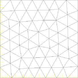
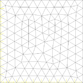
Figure 1. Two initial meshes for the unit square with $68$ nodes (left) and $139$ nodes (right).

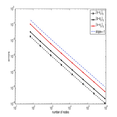
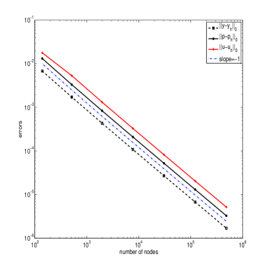
Figure 2. Errors of the multilevel correction algorithm for the discretised optimal state $y_{h}$, adjoint state $p_{h}$ and optimal control $u_{h}$ of Example 5.1 (the left figure corresponds to the left mesh in Figure 1 with 68 nodes as the initial mesh and $7$ uniform refinements with $\beta=2$, the right figure corresponds to the right mesh in Figure 1 with $139$ nodes as the initial mesh and 6 uniform refinements with $\beta=2$).

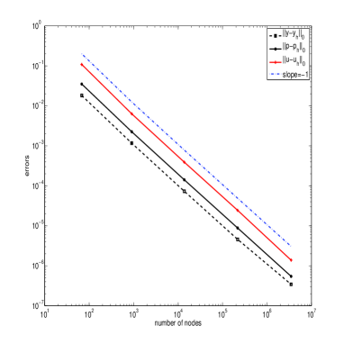
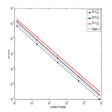
Figure 3. Errors of the multilevel correction algorithm for the discretised optimal state $y_{h}$, adjoint state $p_{h}$ and optimal control $u_{h}$ of Example 5.1 (the left figure corresponds to the left mesh in Figure 1 with 68 nodes as the initial mesh and $4$ uniform refinements with $\beta=4$, the right figure corresponds to the right mesh in Figure 1 with $139$ nodes as the initial mesh and 4 uniform refinements with $\beta=4$).

In the second example, we consider the following optimal controls of semilinear elliptic equation:

$$\min\limits_{u\in U_{ad}}\ \ J(y,u)={1\over 2}\|y-y_{d}\|_{0,\Omega}^{2}+\frac{\alpha}{2}\|u\|_{0,\Omega}^{2}$$

subject to

(5.10) $$\left\{\begin{array}[]{llr}-\Delta y+y^{3}=f+u&\mbox{in}\ \Omega,\\ \ y=0&\mbox{on}\ \partial\Omega,\\ a(x)\leq u(x)\leq b(x)&\mbox{a.e.\ in}\ \Omega.\end{array}\right.$$

Example 5.2.

We set $\Omega=[0,1]^{2}$. Let $a=0$, $b=3$, $\alpha=0.01$, $g_{1}(x_{1},x_{2})=2\pi^{2}\sin(\pi x_{1})\sin(\pi x_{2})$, $g_{2}(x_{1},x_{2})=\sin^{3}(\pi x_{1})\sin^{3}(\pi x_{2})$. Then $f$ is chosen as

(5.14) $$f(x_{1},x_{2})=\left\{\begin{array}[]{llr}g_{1}(x_{1},x_{2})+g_{2}(x_{1},x_{2})-a,&g_{1}(x_{1},x_{2})<a;\\ g_{2}(x_{1},x_{2}),&a\leq g_{1}(x_{1},x_{2})\leq b;\\ g_{1}(x_{1},x_{2})+g_{2}(x_{1},x_{2})-b,&g_{1}(x_{1},x_{2})>b.\end{array}\right.$$

Due to the state equation (5.10), we obtain the exact optimal control $u$

(5.18) $$u(x_{1},x_{2})=\left\{\begin{array}[]{llr}a,&g_{1}(x_{1},x_{2})<a;\\ g_{1}(x_{1},x_{2}),&a\leq g_{1}(x_{1},x_{2})\leq b;\\ b,&g_{1}(x_{1},x_{2})>b.\end{array}\right.$$

We also have

$$y(x_{1},x_{2})=\sin(\pi x_{1})\sin(\pi x_{2}),$$

$$p(x_{1},x_{2})=-2\pi^{2}\alpha\sin(\pi x_{1})\sin(\pi x_{2}).$$

The desired state is given by

$$y_{d}(x_{1},x_{2})=y(x_{1},x_{2})-3y^{2}p+4\pi^{4}\alpha\sin(\pi x_{1})\sin(\pi x_{2}).$$

We solve this nonlinear optimisation problem with standard SQP method (see [8]). We test our proposed multilevel correction algorithm for the above nonlinear optimal control problems on the sequence of multilevel meshes. We use the same sequence of meshes generated with $\beta=2$ as in the first example. It is also observed that second order convergence rate holds for $y_{h}$, $p_{h}$ and $u_{h}$ in the nonlinear case. We remark that the solutions by the multilevel correction method are almost the same as the results by the direct optimization problem solving on the same meshes.

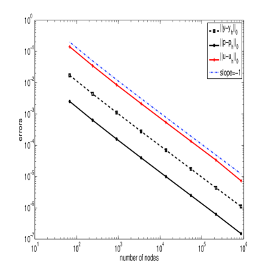
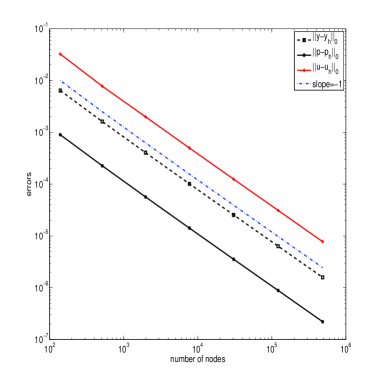
Figure 4. Errors of the multilevel correction algorithm for the discretised optimal state $y_{h}$, adjoint state $p_{h}$ and optimal control $u_{h}$ of Example 5.2 (the left figure corresponds to the left mesh in Figure 1 with 68 nodes as the initial mesh and $7$ uniform refinements, the right figure corresponds to the right mesh in Figure 1 with $139$ nodes as the initial mesh and 6 uniform refinements).

6. Concluding remarks

In this paper, we introduce a type of multilevel correction scheme to solve the optimal control problem. The idea here is to use the multilevel correction method to transform the solution of the optimal control problem on the finest finite element space to a series of solutions of the corresponding linear boundary value problems which can be solved by the multigrid method and a series of solutions of optimal control problems on the coarsest finite element space. The optimal control problem solving is more difficult than the linear boundary value problem solving which has already many efficient solvers. Thus, the proposed method can improve the overall efficiency for the optimization problem solving. With the complexity analysis, we can find that the multilevel correction scheme can obtain the optimal finite element approximation by the almost optimal computational work [20, 21].

We can replace the multigrid method by other types of efficient solvers such as algebraic multigrid method and the domain decomposition method. Furthermore, the framework here can also be coupled with the parallel method and the adaptive refinement technique. The ideas can be extended to other types of linear and nonlinear optimal control problems.

References

- [1] N. Arada, E. Casas and F. Tröltzsch, Error estimates for the numerical approximation of a semilinear elliptic control problem, Comput. Optim. Appl., 23 (2002), pp. 201-229.
- [2] S. Brenner, L. Scott, The Mathematical Theory of Finite Element Methods, Springer-Verlag, New York, 1994.
- [3] A. Borzi and V. Schulz, Multigrid methods for PDE optimization, SIAM Review, 51 (2009), pp. 361-395.
- [4] F. S. Falk, Approximation of a class of optimal control problems with order of convergence estimates, J. Math. Anal. Appl. 44 (1973), pp. 28-47.
- [5] T. Geveci, On the approximation of the solution of an optimal control problem governed by an elliptic equation, RAIRO Anal. Numer., 13 (1979), pp. 313-328.
- [6] M. Hintermüller, K. Ito and K. Kunisch, The primal-dual active set strategy as a semismooth Newton method, SIAM J. Optim., 13 (2003), pp. 865-888.
- [7] M. Hinze, A variational discretization concept in control constrained optimization: The linear-quadratic case, Comput. Optim. Appl., 30 (2005), pp. 45-63.
- [8] M. Hinze, R. Pinnau, M. Ulbrich, S. Ulbrich, Optimization with PDE Constraints, Math. Model. Theo. Appl., 23, Springer, New York, 2009.
- [9] M. Hinze, M. Vierling, The semi-smooth Newton method for variationally discretized control constrained elliptic optimal control problems: implementation, convergence and globalization, Optim. Methods Softw., 27 (2012), no. 6, pp. 933-950.
- [10] A. Kröner, B. Vexler, A priori error estimates for elliptic optimal control problems with a bilinear state equation, J. Comput. Appl. Math., 230 (2009), no. 2, pp. 781-802.
- [11] R. Li, On multi-mesh H-adaptive methods, J. Sci. Comput., 24 (2005), no. 3, pp. 321-341.
- [12] Q. Lin, H. Xie, A multi-level correction scheme for eigenvalue problems, Math. Comput., http://dx.doi.org/10.1090/S0025-5718-2014-02825-1.
- [13] J. L. Lions, Optimal Control of Systems Governed by Partial Differential Equations, Springer-Verlag, New York-Berlin, 1971.
- [14] W. Liu, N. Yan, A posteriori error estimates for optimal boundary control, SIAM J. Numer. Anal., 39 (2001), pp. 73-99.
- [15] W. Liu, N. Yan, A posteriori error estimates for distributed convex optimal control problems, Adv. Comput. Math., 15 (2001), pp. 285-309.
- [16] W. Liu, N. Yan, Adaptive Finite Element Methods for Optimal Control Governed by PDEs, Science Press, Beijing, 2008.
- [17] C. Meyer, R. Rösch, Superconvergence properties of optimal control problems, SIAM J. Control Optim., 43 (2004), pp. 970-985.
- [18] I. Neitzel, B. Vexler, A priori error estimates for space-time finite element discretisation of semilinear parabolic optimal control problems, Numer. Math., 120 (2012), pp. 345-386.
- [19] V. V. Shaidurov, Multigrid Methods for Finite Elements, Kluwer Academic Publics, Netherlands, 1995.
- [20] H. Xie, A type of multilevel method for the Steklov eigenvalue problem, IMA J. Numer. Anal., 34 (2014), no. 2, pp. 592-608.
- [21] H. Xie, A multigrid method for eigenvalue problem, J. Comput. Phys., 274 (2014), pp. 550-561.