Thermodynamics of noninteracting bosonic gases in cubic optical lattices versus ideal homogeneous Bose gases

Abstract

We have studied thermodynamic properties of noninteracting gases in periodic lattice potential at arbitrary integer fillings and compared them with that of ideal homogeneous gases. Deriving explicit expressions for thermodynamic quantities and performing exact numerical calculations we have found that the dependence of e.g. entropy and energy on the temperature in the normal phase is rather weak especially at large filling factors. In the Bose condensed phase their power dependence on the reduced temperature is nearly linear, which is in contrast to that of ideal homogeneous gases. We evaluated the discontinuity in the slope of the specific heat which turned out to be approximately the same as that of the ideal homogeneous Bose gas for filling factor $\nu=1$. With increasing $\nu$ it decreases as the inverse of $\nu$. These results may serve as a checkpoint for various experiments on optical lattices as well as theoretical studies of weakly interacting Bose systems in periodic potentials being a starting point for perturbative calculations.

I Introduction

Inter-particle interactions play a crucial role in fundamental physics. It is well known that, coupling constants of interactions between elementary particles are set and fixed by nature whereas that of atoms, especially in ultracold gases, can be varied in a large scale by using Feshbach resonances feshbach . This gives an opportunity to change even the sign of the s- wave scattering length, $a_{s}$, or to create a system of an ultracold Bose gas with extremely weak interaction. A good example is ${}^{39}K$. Recently roatiprl the non-interacting Bose - Einstein condensate (BEC) has been created by sympathically cooling a cloud of interacting ${}^{39}K$ atoms in an optical trap, and then $a_{s}$ is tuned almost to zero by means of Feshbach resonance, in order to study effects of disorder. In general, experimental and theoretical studies of ideal quantum gases can shed new light on the interdisciplinary phenomenon of Anderson localization Roatinature and a matter - wave interferometry 8roati , opening new directions towards Heisenberg-limited interferometry 9roati . So, study of noninteracting Bose gases in optical traps bailier80 or in optical lattices bailie80 has not only academic interest but also a practical one. In present work we study thermodynamics of noninteracting bosonic gases in cubic optical lattices both in the BEC and normal phases.

Ultracold bosonic atoms in optical lattices have sparked investigations of strongly correlated many-body quantum phases with ultracold atoms lewenstein that are now at the forefront of current researches. They may be used as quantum emulations of more complex condensed matter system, and may greatly facilitate the achievements of the quantum Hall regime for the ultracold atomic gases NCOOPER . Experimentally they are created by superimposing two counter-propagating laser beams of the same wavelength and frequency that act as an periodic potential. In the simplest case, when the depth is constant and isotropic the potential can be represented as follows:

$$\small V_{L}({\bf r})=V_{0}\sum_{\alpha=1}^{d}\sin^{2}(k_{0}^{\alpha}r_{\alpha}),$$ (1)

where the wave vector ${\bf k}_{0}\equiv\{k_{0}^{\alpha}\}$ is related to the laser wavelength $\lambda_{\alpha}$ as $k_{0}^{\alpha}=2\pi/\lambda_{\alpha}$, and $d$ is the space dimension of a cubic lattice, $d=1,2,3$.

It is well known that, an ideal homogeneous Bose (IHB) gas of noninteracting atoms consists of free atoms with the plane wave $\exp(i{\bf k}{\bf r})$, and with the energy dispersion relation $\epsilon_{k}={\bf k}^{2}/2m$. The creation of an optical lattice may be considered as a procedure of loading preliminarily magnetically trapped ultracold Bose atoms into a well tuned laser field, whose influence on the atoms, being in fact the Stark effect, is simulated via periodic potential (1). Now the dispersion is no longer quadratic with the momentum, but develops gaps at specific locations determined by the lattice structure. This energy can be specified by a band index and a quasimomentum, taking on values within the first Brillouin zone only. As to the wave function it can be written as a Bloch function $\chi_{nk}({\bf r})=\sum_{i}\exp(i{\bf k}{\bf r})\omega_{n}({\bf r}-{\bf r}_{i})$ in the Wannier representation. In the limit $V_{0}\gg E_{R}$, where $E_{R}$ is the recoil energy, each well of the periodic potential supports a number of vibrational levels, separated by an energy $\omega_{0}\gg E_{R}$. At low temperatures, atoms are restricted to the vibrational level at each site. Their kinetic energy is then frozen, except for the small tunneling amplitude to neighboring sites. The associated single particle eigenstates in the lowest band are Bloch waves with quasimomentum ${{\bf k}}$ and energy

$$\small\epsilon_{0}({\bf k})=3/2\omega_{0}-2J[\cos(k_{x}a)+\cos(k_{y}a)+\cos(k_{z}a)]+\ldots$$ (2)

where $\omega_{0}$ is the energy of local oscillations in the well zwerger . This is one of the main differences between IHB gas and noninteracting Bose gas in optical lattices, which is no longer homogeneous either. The bandwidth parameter $J>0$ is the gain in the kinetic energy due to the nearest neighbor tunneling, which can be approximated as

$$\small J\approx\displaystyle\frac{4}{\sqrt{\pi}}E_{R}\exp\left[-2\sqrt{\displaystyle\frac{V_{0}}{E_{R}}}\right]\left[{\displaystyle\frac{V_{0}}{E_{R}}}\right]^{3/4}$$ (3)

where $E_{R}=k_{0}^{2}/{2m}$ , $k_{0}=\mid{\bf k}_{0}\mid$ is the laser wave vector modulus, $k_{0}=\pi/a$, $a$ is the lattice spacing.

By the assumption that the only lowest band is taken into account, an optical lattice without harmonic trap can be described by the Bose-Hubbard model stoofbook ,

$$\small\hat{H}=-J\sum_{\langle i,j\rangle}(\hat{b}_{i}^{+}\hat{b}_{j}+hc)+\frac{U}{2}\sum_{j}^{N_{s}}\hat{n}_{j}(\hat{n}_{j}-1),$$ (4)

where $\hat{b}_{i}^{+}$ and $\hat{b}_{i}$ are the bosonic creation and annihilation operators on the site $i$; the sum over $\langle i,j\rangle$ includes only pairs of nearest neighbors; $J$ is the hopping amplitude, which is responsible for the tunneling of an atom from one site to another neighboring site; $U$ is the on site repulsion energy, $\hat{n}_{j}$ is the number operator and $N_{s}$ the number of sites. Depending on the ratio $\kappa=U/J$ , the filling factor $\nu$ and the temperature $T$, the system may be in superfluid, Mott insulator or in normal $(N)$ phases. Note that, strictly speaking the Mott insulator phase may be reached only for $T=0$ and commensurate, i.e. integer filling factors Yukalovobsor , $\nu=N/N_{s}$, where $N$ total number of atoms. The filling factor is related to the average atomic density, $\rho=N/V$ as $\nu=\rho a^{d}$, where $V$ - volume of the system occupied with the atoms.

We shall study the system with $\kappa=0$ described by the Hamiltonian (4) taking into account only the lowest band with the dispersion (2). Since an ideal gas with the quadratic spectrum at small momentum, i.e. $\epsilon(k)=ck^{2}+O(k^{3})$ can not exhibit superfluidity landau , our discussions will concern the phase transition from BEC phase into a normal phase.

On the other hand properties of $3d$ a homogeneous Bose gas of noninteracting atoms are well known and outlined in textbooks landau ; huang . Particularly, following facts are well established:

• At sufficiently low temperatures they exhibit a phase transition from normal to Bose Einstein state with the critical temperature

  $$\small{\tilde{T}}_{c}^{0}=\displaystyle\frac{2\pi}{m}\left[\displaystyle\frac{\tilde{\rho}}{g_{3/2}(1)}\right]^{2/3}$$ (5)

  where $g_{\sigma}(z)=1/\Gamma(\sigma)\int_{0}^{\infty}x^{(\sigma-1)}dx/(\exp(x)z^{-1}-1)$ is a Bose function, $m$ is the atomic mass. Here and below we denote by tilde the quantities characterizing the IHB gases and use the units $\hbar=1$, $k_{B}=1$. At the critical temperature such quantities as the energy - $E(T)$, entropy - S(T) and the specific heat, $C_{v}=(\partial E/\partial T)_{v}$ are continuous, while the derivative of $C_{v}$ with respect to the temperature $\partial C_{v}/\partial T$ has a discontinuity given by

  $$\small{\tilde{\Delta}}=\displaystyle\frac{{\tilde{T}}_{c}^{0}}{N}\left[\left(\displaystyle\frac{\partial{\tilde{C}}_{v}}{\partial T}\right)_{\tilde{T}_{c}^{-}}-\left(\displaystyle\frac{\partial{\tilde{C}}_{v}}{\partial T}\right)_{\tilde{T}_{c}^{+}}\right]=3.66$$ (6)

  where $N$ is the total number of particles.

• The critical temperature, ${\tilde{T}}_{c}^{0}$ , divides the scale of temperature into two different regimes: BEC and normal. In the BEC phase, $T\leq{\tilde{T}}_{c}^{0}$ when the chemical potential of the gas is zero i.e. $\mu=0$, the energy and the specific heat behave as ${\tilde{E}}/N\sim(T/{\tilde{T}}_{c}^{0})^{5/2}$, ${\tilde{C}}_{v}/N\sim(T/{\tilde{T}}_{c}^{0})^{3/2}$ which can be shown analytically huang .

• The thermodynamic quantities exhibit a scale invariance, which means that they depend explicitly on the reduced temperature $t=T/{\tilde{T}}_{c}^{0}$, but not on the density. One may find in the literature good approximations for e.g. ${\tilde{E}}(t)$ or ${\tilde{C}}_{v}(t)$ wang . Moreover, there is a simple scale relation between the internal energy and the pressure ${\tilde{P}}$:

  $$\small{\tilde{E}}(t)=\displaystyle\frac{d}{2}{\tilde{P}}(t)V$$ (7)

  which holds for IHB gas exactly both in the BEC and normal phases mancarella .

Now one may assume that IHB gas is loaded into an optical lattice. Mathematically this means that a periodic potential is implemented as an external potential given by Eq. (1). Clearly, the presence of this potential will change the energy dispersion and makes a boundary for the quasimomentum ${\bf k}$. So, the bare dispersion is no longer quadratic $\epsilon_{k}={\bf k}^{2}/2m$ with $k=0\div\infty$ and the quasimomentum integration is taken only within the first Brillouin zone , $k_{\alpha}\in[-\frac{\pi}{a},\frac{\pi}{a}]$. Then, how the properties of noninteracting Bose gas, in particularly, listed above, will be changed due to the periodic potential? In present work we shall make an attempt to answer these questions and make the parallel between the thermodynamic properties IHB and optically confined gases. The results will be useful in studying optical lattices with a weak interaction and may serve as a check point for further theoretical studies.

We shall study high filling region $(\nu>3)$ also. This region is actual to investigate inteference and coherence properties of BEC, as well as properties of number squeezed states weli . Note that an experimental realization of optical lattice with high filling factor is rather difficult. Although one dimensional optical lattice with $\nu=100$ polkovnikov or array of condensates with $\nu=10^{4}$ has been created recently hajibaba actual three dimensional opticall lattice has no more than three atoms per site bloch .

This paper is organized as follows. In Sec. II we derive main equations for thermodynamic quantities of ideal optical lattices which will serve as a working formulas in the next sections. In Sec. III we discuss the power dependence of condensate fraction on the reduced temperature. In Secs. IV and V the $T$ and $\nu$ dependence of the entropy and energy will be studied. We study the heat capacity and its derivative in Sec. VI. The Sec. VII will discuss the stability properties. Our conclusions are brought in the last VIII section. In Appendix A and B we present useful formulas for IHB gases and ideal optical lattices respectively.

II Thermodynamic quantities: general relations

The thermodynamic potential of the noninteracting Bose gas in an optical lattice is given by ourknr2 ; ourknr1

$$\small\Omega=T\sum_{q}\ln\left[1-ze^{-\beta\varepsilon(q)}\right]$$ (8)

where $\beta=1/T$, $\varepsilon(q)=2J\displaystyle\sum_{\alpha=1}^{3}(1-\cos\pi q_{\alpha})$ - bare dispersion, $z=\exp(\beta\mu)$ - fugacity, and $\sum_{q}f(q)\equiv N_{s}\int_{0}^{1}dq_{1}dq_{2}dq_{3}f(q)$ . Note that in (8) the chemical potential $\mu$ includes the term $6J$, Yukalovobsor which is not written here explicitly.

From (8) one may find all needed thermodynamic quantities, namely

• Number of particles:

  $$\small N=-\left(\displaystyle\frac{\partial\Omega}{\partial\mu}\right)_{T}=\sum_{q}\displaystyle\frac{1}{z^{-1}e^{\beta\varepsilon(q)}-1}$$ (9)

• Entropy:

  $$\small S=-\left(\displaystyle\frac{\partial\Omega}{\partial T}\right)_{\mu}=-\beta\left[\Omega+\sum_{q}\displaystyle\frac{(\mu-\varepsilon(q))}{z^{-1}e^{\beta\varepsilon(q)}-1}\right]$$ (10)

• Energy:

  $$\small E=TS+N\mu+\Omega=\sum_{q}\displaystyle\frac{\varepsilon(q)}{z^{-1}e^{\beta\varepsilon(q)}-1}$$ (11)

• Pressure:

  $$\small P=-\displaystyle\frac{\Omega}{V}=-\displaystyle\frac{\Omega}{a^{d}N_{s}}$$ (12)

• Fugacity. Actually in the BEC phase $z(T\leq T_{c}^{0})=1$. In the normal phase the function $z(T)$ may be found by solving (9) with respect to $z$ for given temperature T and filling factor. To calculate the specific heat one needs also $z^{\prime}=(\partial z/\partial T)_{\rho}$. To obtain an explicit expression for $z^{\prime}$ , we differentiate both sides of (9) for a fixed $N$ and solve the equation $dN/dT=0$ with respect to $z^{\prime}$ pathria . The result is:

  $$\small z^{\prime}=-\displaystyle\frac{zR_{112}(z,T)}{TR_{012}(z,T)}$$ (13)

  where we introduced following integrals

  $$\small\begin{array}[]{l}R_{ijk}(z,T)=\displaystyle\frac{1}{N_{s}}\sum_{q}\displaystyle\frac{(\beta\varepsilon(q))^{i}e^{j\beta\varepsilon(q)}}{\left[e^{\beta\varepsilon(q)}z^{-1}-1\right]^{k}}\equiv\int_{0}^{1}dq_{1}dq_{2}dq_{3}\displaystyle\frac{x^{i}e^{jx}}{\left[e^{x}z^{-1}-1\right]^{k}},\\ x=\beta\varepsilon(q)\end{array}$$ (14)

  Below we omit $T$ dependence of this function for simplicity, setting $R_{ijk}(z)\equiv R_{ijk}(z,T)$. Note that in the case of IHB gases the analogous integrals may be rewritten more compactly in terms of Bose functions $g_{\sigma}(z)$ due to the recurrent relations (A.3).

• Heat capacity, $C_{v}=(\partial E/\partial T)_{V}$. Differentiating (11) and using (13), (14) one obtains

  $$\small C_{v}/N_{s}=\left\{\begin{array}[]{ll}R_{212}(1)&(T\leq{T_{c}^{0}})\\ \\ \displaystyle\frac{R_{212}(z)R_{012}(z)-R_{112}^{2}(z)}{zR_{012}(z)}&\quad(T>{T_{c}^{0}})\end{array}\right.$$ (15)

  Note that, the heat capacity per particle $C_{v}/N$ may be evaluated by dividing these expressions to $\nu$ i.e. $C_{v}/N=[C_{v}/N_{s}]/\nu$.

• The derivative of the specific heat: $(\partial C_{v}/\partial T)$. From (15) one may obtain

  $$\small\displaystyle\frac{T}{N_{s}}\left(\displaystyle\frac{\partial C_{v}}{\partial T}\right)_{T\leq{T_{c}^{0}}}=2R_{323}(1)-2R_{212}(1)-R_{312}(1)$$ (16)

  in the BEC phase and a rather long expression

  $$\small\begin{array}[]{l}\displaystyle\frac{z^{2}T}{N_{s}}\left(\displaystyle\frac{\partial C_{v}}{\partial T}\right)_{T>{T_{c}^{0}}}=2R_{323}(z)-2zR_{212}(z)-zR_{312}(z)+\\ \\ \displaystyle\frac{R_{112}(z)[2zR_{112}(z)+3zR_{212}(z)-6R_{223}(z)]}{R_{012}(z)}-\\ \\ \displaystyle\frac{2R_{112}^{2}(z)[zR_{112}(z)-3R_{123}(z)]}{R_{012}^{2}(z)}-2R_{112}^{3}(z)\left[\displaystyle\frac{R_{023}(z)}{R_{012}^{3}(z)}\right]\end{array}$$ (17)

  in the normal phase where we used Eqs. (13) and (14).

III The critical temperature and the condensed fraction

For a noninteracting gas the phase transition BEC $\to N$ occurs when $\mu\rightarrow 0$, so that the critical temperature ${T_{c}^{0}}$ is determined by the following equation with a given filling factor $\nu_{c}$:

$$\small\nu_{c}=\int_{0}^{1}dq_{1}dq_{2}dq_{3}\displaystyle\frac{1}{e^{\varepsilon(q)/{T_{c}^{0}}}-1}$$ (18)

which directly follows from Eq. (9). The similar equation for IHB gas can be solved analytically giving $\tilde{T}_{c}^{0}\sim\rho^{2/3}$ power dependence as it was outlined above. However, for an ideal optical lattice the Eq.(18) can not be solved analytically, so an explicit dependence of ${T_{c}^{0}}(\nu)$ on the filling factor, which plays the role of density, $\nu=a^{3}\rho$ may be found by studying numerical solutions of (18). We have recently shown ouriman1 that the function ${T_{c}^{0}}(\nu)$ may be approximated as

$$\small{T_{c}^{0}}(\nu)=3.96J\nu e^{0.37/\nu}$$ (19)

Particularly, ${T_{c}^{0}}(\nu)$ has a linear dependence on $\nu$ at large filling factors $(\nu\geq 5)$ as it is seen from Fig.1. This figure illustrates also the fact that the critical temperature of an ideal gas is strongly modified by the influence of the periodic potential, especially at large filling factors. Note that a magnetic trap with harmonic potential $U(r)=m(\omega_{x}^{2}x^{2}+\omega_{y}^{2}y^{2}+\omega_{z}^{2}z^{2})/2$ also modifies the power dependence of critical temperature as keterle

$$\small{T_{c}^{0}}(mag.trap)=0.94\omega_{0}N^{1/3}$$ (20)

where $\omega_{0}=(\omega_{x}\omega_{y}\omega_{z})^{1/3}$ is the geometric average of trap frequencies.

The condensed fraction $n_{0}=N_{0}/N$, where $N_{0}$ is the number of condensed particles, may be defined as

$$\small n_{0}=1-n_{1}$$ (21)

where

$$\small n_{1}=\displaystyle\frac{1}{\nu N_{s}}\sum_{q}\displaystyle\frac{1}{e^{\beta\varepsilon(q)}-1}=\displaystyle\frac{1}{\nu}{\displaystyle\int_{0}^{1}dq_{1}dq_{2}dq_{3}}\displaystyle\frac{1}{e^{\beta\varepsilon(q)}-1}$$ (22)

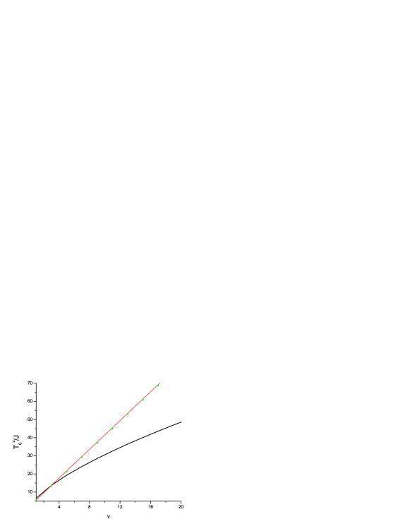
Figure 1: (Color online) The condensation temperature in units $J$ as a function of the filling factor calculated from Eq. (19) (thin solid line). The symbols correspond to the exact solutions of Eq.(18). The thick solid line corresponds to the critical temperature of IHB gas with an effective mass $m=1/2Ja^{2}$ and density $\rho=\nu/a^{3}$ exhibiting a power law $\nu^{2/3}$.

The function $n_{0}(t,\nu)$, for various values of $\nu$ and the reduced temperature $t=T/{T_{c}^{0}}$ is presented in Fig.2.

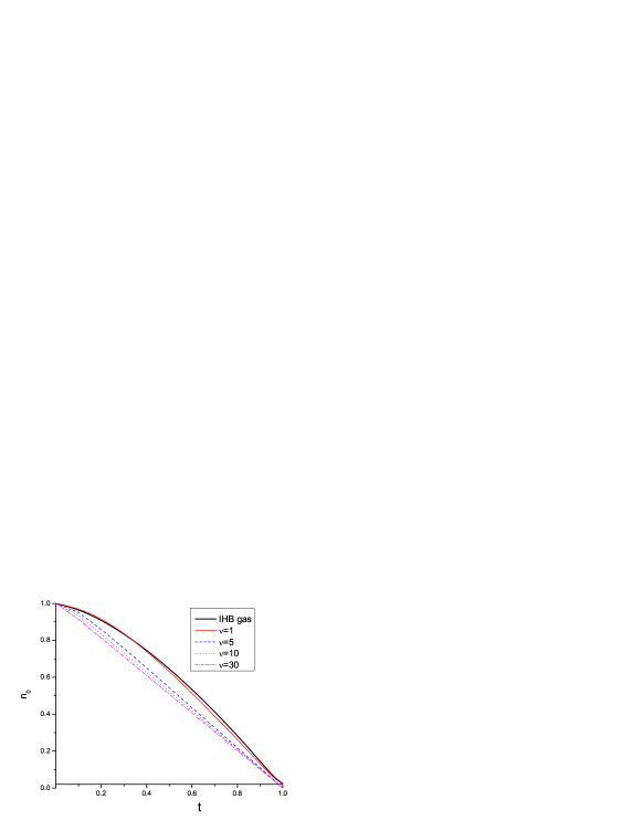
Figure 2: (Color online) The condensed fraction $n_{0}$ vs reduced temperature $t=T/T_{c}^{0}$, as an exact solution of Eqs. (21) and (22) for different values of $\nu$. The thick solid line corresponds to the ideal homogeneous Bose gas given by (23).

It is seen from Fig.2 that at $\nu=1$ the temperature dependence the condensed fraction in both cases is almost the same:

$$\small n_{0}(t,\nu)\mid_{\nu=1}\sim{\tilde{n}}_{0}(t)=1-t^{3/2}$$ (23)

However, with the increasing of the filling factor, say, $(\nu\geq 5)$ , $n_{0}(t,\nu)$ approaches to a linear function of temperature i.e.

$$\small n_{0}(t,{\nu\geq 5})\sim 1-t.$$ (24)

IV Some scaling properties

IV.1 Ideal homogenious Bose gas

In general, in the thermodynamic limit, $(N\rightarrow\infty$, $V\rightarrow\infty$, $\rho=N/V\neq\infty)$ any thermodynamic quantity of IHB gas in the equilibrium is a function of two independent variables, the temperature and the density , i.e. , $W=W(T,\rho)$ .

It is easy to prove following statement: Let $W(T,\rho)$ of a nonrelativistic IHB gas has a dimensionality as $[W]=(Energy)^{n}(space)^{3l}$. Then $W(T,\rho)$ may be represented as

$$\small W(T,\rho)=(\tilde{T}_{c}^{0})^{n}\rho^{-l}{W^{\prime}}(t)$$ (25)

where $W^{\prime}(t)$ is the function of only reduced temperature, regardless of the particle mass $m$.
Proof . Since the most of quantities may be derived from the thermodynamic potential, it is enough to prove this statement for $\Omega(T,\rho):$

$$\small\Omega=VT\displaystyle\int\displaystyle\frac{d{{\bf k}}}{(2\pi)^{3}}\ln\left[1-ze^{-\varepsilon({\bf k})/T}\right]$$ (26)

where $\varepsilon({\bf k})={\bf k}^{2}/2m$. Making following substitution in the integral

$$\small k=\sqrt{2\tilde{T}_{c}^{0}mtx},\quad\quad x=0..\infty$$ (27)

and integrating by parts one obtains:

$$\small\begin{array}[]{l}\Omega=-\displaystyle\frac{4TN}{3\tilde{\rho}\lambda_{T}^{3}\sqrt{\pi}}\displaystyle\int_{0}^{\infty}\displaystyle\frac{x^{3/2}dx}{e^{x}\tilde{z}^{-1}-1}=-\displaystyle\frac{NTg_{5/2}(\tilde{z})}{\tilde{\rho}\lambda_{T}^{3}}\end{array}$$ (28)

where $\lambda_{T}=\sqrt{2\pi/mT}$ is the thermal wavelength, and $\tilde{z}$ is the fugacity. On the other hand inverting Eq. (5) gives

$$\small\tilde{\rho}\lambda_{T}^{3}=\zeta(3/2)t^{-3/2}$$ (29)

where $\zeta(x)$ is the Riemann function. Now inserting (29) into (28) we obtain

$$\small\Omega=-\displaystyle\frac{N\tilde{T}_{c}^{0}t^{5/2}g_{5/2}(\tilde{z})}{\zeta(3/2)}$$ (30)

That is the dimensionless thermodynamic potential per particle $\Omega^{\prime}/N$ may be presented as a function only of $t$:

$$\small\displaystyle\frac{{\Omega^{\prime}}(t)}{N}=-\displaystyle\frac{t^{5/2}g_{5/2}(\tilde{z})}{\zeta(3/2)}$$ (31)

At the first glance it seems that, the remaining explicit $\tilde{\rho}$ or $m$ dependence may come from $\tilde{z}$. However, it can be shown that $\tilde{z}$ satisfies the above statement by itself: $\tilde{z}(T,\rho)=\tilde{z}(t)$. In fact, the equation

$$\small\tilde{\rho}=\displaystyle\int\displaystyle\frac{d{{\bf k}}}{(2\pi)^{3}}\displaystyle\frac{1}{\tilde{z}^{-1}e^{\varepsilon({\bf k})/T}-1}$$ (32)

which defines $\tilde{z}$, may be, clearly, rewritten as

$$\small\tilde{\rho}\lambda_{T}^{3}=g_{3/2}(\tilde{z})$$ (33)

Now from Eqs. (29) and (33) we get

$$\small g_{3/2}(\tilde{z})=\zeta(3/2)t^{-3/2}$$ (34)

Thus $\tilde{z}(T,\rho)=\tilde{z}(t)$, and hence the density dependence of e.g. $\Omega^{\prime}$ is involved only via the reduced temperature as $t\sim T/\tilde{\rho}^{2/3}$.

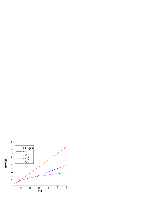
Figure 3: (Color online) This relation between the internal energy and the thermodynamic potential, $\mid\Omega\mid$, equals exactly to unity for ideal homogeneous Bose gas, as presented by the thick solid line (see Eq.s (A.6) and (A.10) )

Note that in the above discussions we didn’t lose the number of free parameters. Actually, there are two independent variables: on the LHS of (25) they are $T$ and $\tilde{\rho}$, while on the RHS $T$ and $\tilde{T}_{c}^{0}$.

Similarly, it can be easily shown that

$$\small\begin{array}[]{l}\displaystyle\frac{\tilde{E}^{\prime}(t)}{N}=\displaystyle\frac{3t^{5/2}g_{5/2}(\tilde{z})}{2\zeta(3/2)}\\ \\ \displaystyle\frac{\tilde{S}^{\prime}(t)}{N}=\displaystyle\frac{5t^{3/2}g_{5/2}(\tilde{z})}{2\zeta(3/2)}\\ \\ {\tilde{P}^{\prime}(t)}=\displaystyle\frac{t^{5/2}g_{5/2}(\tilde{z})}{\zeta(3/2)}\end{array}$$ (35)

where $\tilde{P}(t)^{\prime}={\tilde{P}}/\tilde{T}_{c}^{0}\rho$ (see Appendix A).

IV.2 Ideal optical lattice

The natural question arises, if a thermodynamic quantity of an ideal optical lattice satisfies the scale relation given in (25), where the role of the density plays the filling factor $\nu=\rho a^{3}$? To answer this question we consider the BEC and the normal phases separately.

In the BEC phase the thermodynamic potential per site is given by

$$\small\Omega(T\leq{T_{c}^{0}})/N_{s}=Ta^{3}\displaystyle\int_{-\pi/a}^{\pi/a}\displaystyle\frac{dk_{1}dk_{2}dk_{3}}{(2\pi)^{3}}\ln\left[1-ze^{-\varepsilon({\bf k})/T}\right]_{z=1}$$ (36)

where $\varepsilon({\bf k})=2J\displaystyle\sum_{\alpha=1}^{3}(1-\cos(k_{\alpha}a))$. The Eq. (36) displays that in this phase $\Omega(T)/N_{s}$ absolutely does not dependent on $\nu$. So, it can be represented as a function of the reduced temperature $t$ as: $\Omega(T\leq{T_{c}^{0}})/N_{s}=\Omega(t{T_{c}^{0}})/N_{s}$ and hence the thermodynamic potential per particle behaves as $\Omega(T)/N\sim 1/\nu$, due to the relation $\nu N_{s}=N$.

In the normal phase an explicit $\nu$ dependence of all thermodynamic quantities comes from the function $z(t,\nu)$. To illustrate the fact that in contrast to the fugacity of IHB gas, the fugacity of a noninteracting gas in the periodic potential dependence not only on $t$ but also on $\nu$ we will use a simple Debay approximation (see Appendix B). So, on the one hand

$$\small\nu=a^{3}\displaystyle\int_{-\pi/a}^{\pi/a}\displaystyle\frac{dk_{1}dk_{2}dk_{3}}{(2\pi)^{3}}\displaystyle\frac{1}{z^{-1}e^{\varepsilon(k)/T}-1}\simeq a^{3}\displaystyle\int_{0}^{k_{D}}\displaystyle\frac{k^{2}dk}{2\pi^{2}}\displaystyle\frac{1}{z^{-1}e^{\varepsilon_{k}/T}-1}$$ (37)

where $\varepsilon_{k}={\bf k}^{2}/2m$, $m=1/2Ja^{2}$, $k_{D}=(6\pi^{2})^{1/3}/a$. On the other hand ${T_{c}^{0}}$ corresponding to this fixed $\nu$ is defined by

$$\small\nu\simeq a^{3}\displaystyle\int_{0}^{k_{D}}\displaystyle\frac{k^{2}dk}{2\pi^{2}}\displaystyle\frac{1}{e^{\varepsilon_{k}/{T_{c}^{0}}(\nu)}-1}$$ (38)

Now equating the last two equations to each other and making following substitution

$$\small k=\sqrt{2mx{T_{c}^{0}}},\quad\quad x=0..x_{D},\quad\quad x_{D}=\displaystyle\frac{6^{2/3}\pi^{4/3}}{2a^{2}m{T_{c}^{0}}(\nu)}$$ (39)

one obtains following equation with respect to $z$

$$\small\displaystyle\int_{0}^{x_{D}}\sqrt{x}dx\left[\displaystyle\frac{1}{z^{-1}e^{x/t}-1}-\displaystyle\frac{1}{e^{x}-1}\right]=0$$ (40)

Although the integrand in Eq. (40) depends only on $t$ the upper boundary of the integral explicitly depends on $\nu$ e.g. through Eq. (19) as ${T_{c}^{0}}\approx 4\nu J$ and as a result $z$ acquires an explicit, nonlinear $\nu$ dependence.

Thus we may conclude that a thermodynamic quantity describing an ideal optical lattice may be presented as the only function of $T$ in the BEC phase, while in the normal phase, its density dependence cannot be simply extracted as it was done for IHB gas in Eq. (25).

In the content of the scaling, there is a simple scale relation between the internal energy and the pressure ${\tilde{P}}$:

$$\small{\tilde{E}}(t)=\displaystyle\frac{d}{2}{\tilde{P}}(t)V$$ (41)

which holds for IHB gas exactly. In textbooks it is usually derived by the integration by parts of the free energy, ${\tilde{\Omega}}=-{\tilde{P}}V$. On the other hand, it can be shown that mancarella , this relation is a consequence of the scale invariance of the Hamiltonian with respect to the dilation of coordinates such as $r\rightarrow\lambda r$.

To discuss the scaling relation $E=3PV/2$ we plot in Fig.3 dimensionless quantity $3PV/2E$ which equals exactly to unity for IHB gases. It is seen from Fig.3 that the presence of the external potential leads to a strong breaking of this relation irrespective of the values of $\nu$ and $t$.

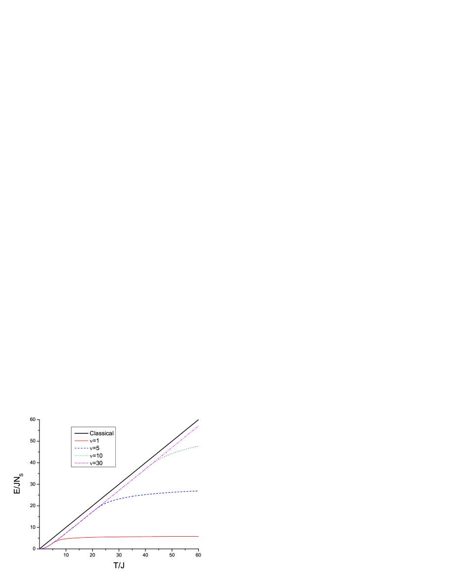
a)

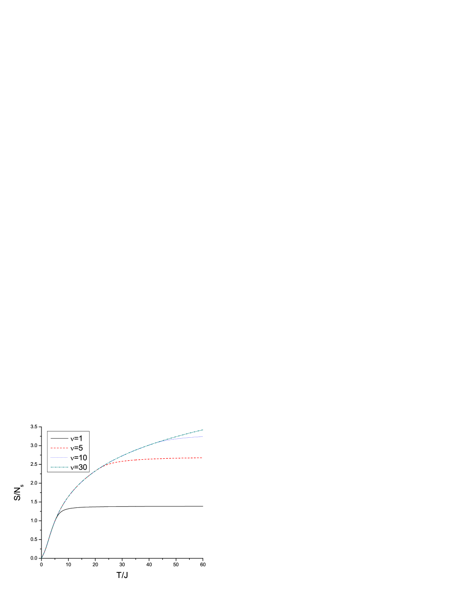
b)

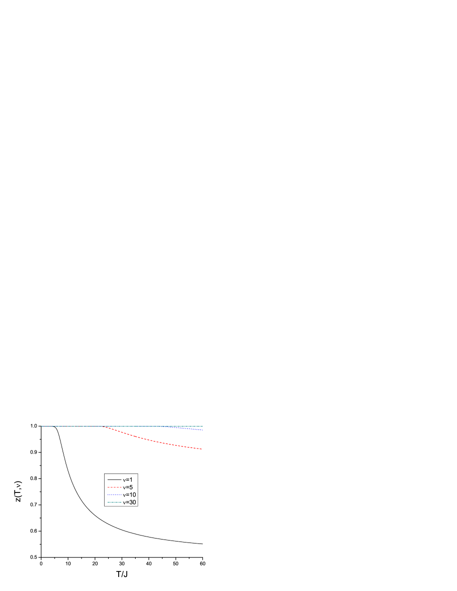
c)

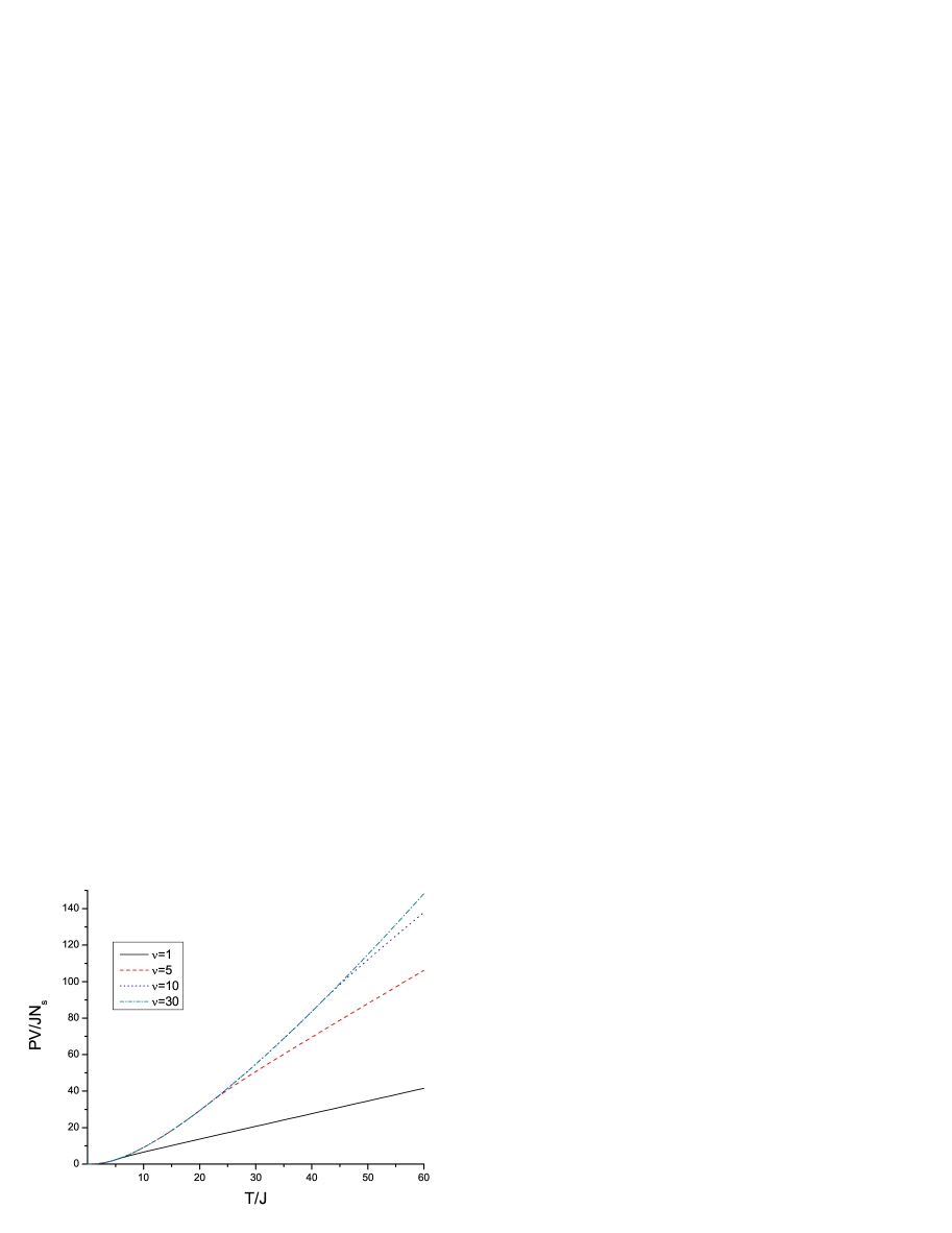
d)

Figure 4: (Color online) The energy per site in units $J$, (a), the entropy per site (b), the fugacity (c) and the absolute value of the thermodynamic potential per site in units $J$, (d) of noninteracting gases in optical gases for different filling factors $\nu$ vs the absolute scale of the temperature $T/J$. The branch points correspond to the following critical temperatures: ${T_{c}^{0}}(1)=5.5911J$, ${T_{c}^{0}}(5)=21.6714J$ and ${T_{c}^{0}}(10)=41.5J$ .

V $T$ and $\nu$ dependence of thermodynamic quantities

To discuss the general tendency of a thermodynamic quantity of an ideal optical lattice as a function of temperature and filling factor we present in Figs. 4 the energy (4a), entropy (4b), fugacity (4c) and the absolute value of thermodynamic potential per site in units $J$ (4d) on the scale of the dimensionless absolute temperature for various $\nu$. The branch points correspond to the following critical temperatures: ${T_{c}^{0}}(1)=5.5911J$, ${T_{c}^{0}}(5)=21.6714J$ and ${T_{c}^{0}}(10)=41.5J$ which separate the BEC and the normal phases. Below we consider these two phases separately.

a)The BEC phase. In this phase these quantities does not depend on $\nu$ as it was shown in the previous section. It is seen from Figs. 4 that for $T\leq{T_{c}^{0}}$ the power dependence of $E(T)$, $S(T)$ and $P(T)$ on temperature is nearly linear e.g. $E(T)\sim T$ . This is similar to the classical gas, as it is illustrated in Fig. 4(a) and in contrast to the case of IHB gas where for instance $S/N\sim T^{3/2}$ (see Appendix A).

b)The normal phase. The difference between the thermodynamic quantities of noninteracting particles in periodic potential and that of IHB gas is rather large for $T>{T_{c}^{0}}$. As it is seen from Figs. 4 (a) and (b) when the temperature reaches its critical value, ${T_{c}^{0}}(\nu)$, the energy and the entropy become quite insensitive to temperature, especially at large filling factors $\nu\geq 5$. Mathematically this tendency may be explained as follows. With the increasing of temperature the exponential function in Eq. (11) fast decreases. On the other hand as it is clearly seen from Fig. 4(c) the factor $z^{-1}$ in this equation also increases exponentially (see Footnote 3). As a result the whole product $\exp(\varepsilon(q)/T)/z(T)$ in Eq. (11) goes to a constant value at large $T$ and $\nu$ as it is displayed in Fig.5(d). For the similar reason the absolute value of the dimensionless thermodynamic potential per site, $|\Omega|/JN_{s}$ plotted in Fig.4(d) increases with the increasing of the temperature, as it is clear from the Eq. (8). Note also that, the pressure (Fig. 4(d)) and module of the chemical potential $|\mu|$ fast increases (Fig. 5(c)) with the increasing of temperature and the density as expected from general physical principles.

To give a further illustration of the contrast between IHB gas and the one in the periodic potential in the normal phase we present in Figs. 5 the energies (a) as well as entropies (b) of both systems on the scale of the reduced temperature. As it is seen from the figures, with the increasing the temperature , for instance, the energy of the IHB gas continues to increase , while that of the ideal optical lattice remains nearly constant. For small filling factors $S(t,\nu)/N$ is almost linear in the temperature. As for the $\nu$ dependence of this function, the entropy decreases as $1/\nu$ with increasing $\nu$. A similar behavior of $S(t,\nu)/N$ was found in Ref. pra69 where the authors studied entropy - temperature curves in a large scale of temperature for $\nu\leq 4$.

It is clear that interatoimic interaction become crucial at large filling factors. Thus our results for $\nu>4$ may be considered just as model calculations.

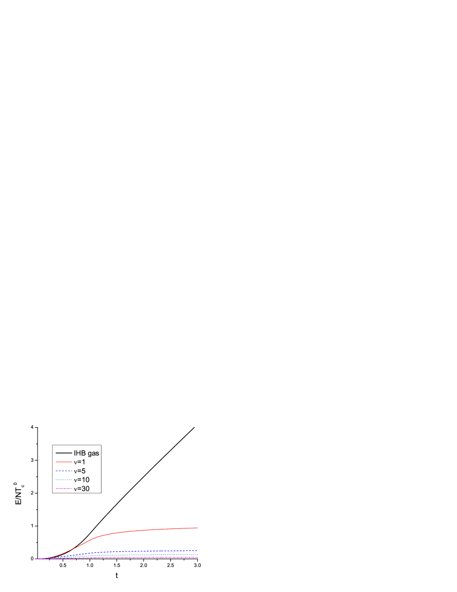
a)

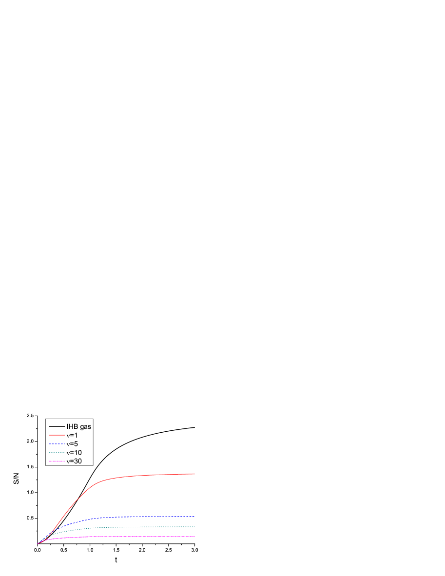
b)

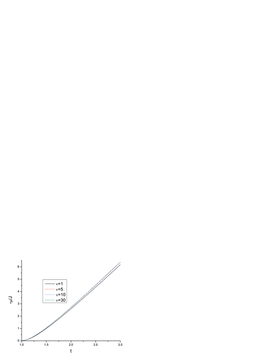
c)

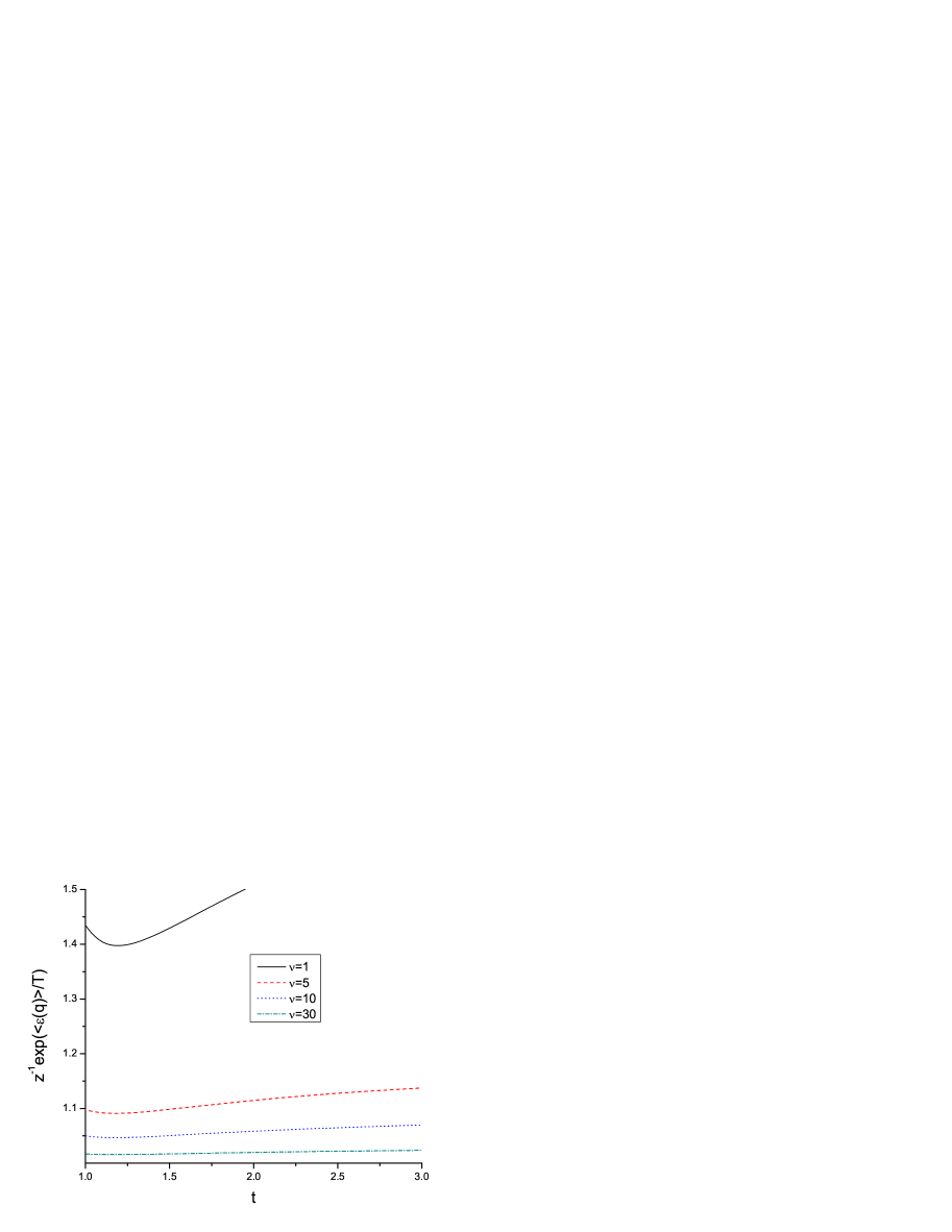
d)

Figure 5: (Color online) The energy in units ${T_{c}^{0}}$ (a), entropy (b) per particle and the absolute value of the chemical potential in units $J$ (c) for different values of $\nu$. In the evaluating of the quantity $z^{-1}\exp(<\varepsilon(q)/T>)$ presented in (d) we set $<\varepsilon(q)=1>$. The thick solid lines in (a) and (b) correspond to the ideal homogeneous Bose gas given by (A.9) and (A.10).

.

VI The specific heat and the jump in $\partial C_{v}/\partial T$

The $\lambda$ - shape behavior of the specific heat per particle for non-interacting bosons for $\nu=1$ has been predicted in Ref. das . Below the case with also large $\nu$ will be considered. The specific heat per site $C_{v}/N_{s}$ and per particle $C_{v}/N$ calculated from Eqs. (15) are presented in Fig.s 6 (a) and (b) respectively. It is seen that $C_{v}(\nu,t)/N_{s}$ reaches unity at rather small values of $t$, say, $t\leq 0.2$ for $\nu\geq 5$ in the BEC phase. In the normal phase the same quantity fast decreases with increasing the temperature that again confirms a weak dependence of the energy on $t$, especially at high temperatures. Moreover at such temperatures the dependence of the function $C_{v}(\nu,t)/N_{s}$ on $\nu$ nearly vanishes (see Fig. 6(a)) and it mostly becomes a function of only $t$, similarly to the specific heat of IHB gas. Therefore $\lambda$ - shaped $C_{v}/N$, i.e. the specific heat per particle , decreases as $C_{v}(\nu,t)/N\sim 1/\nu$ with the increasing $\nu$ and fades out at large $t$, namely at $t\geq 2.3$ in contrast to IHB gas, as it is seen from Fig.6(b).

It is well known that the most of thermodynamic quantities are continuous at the critical temperature for IHB gas. This remains true for optical lattices also, as it is seen from figures Figs.3-Figs.6 . However there is a discontinuity in the slope of the specific heat, $\partial C_{v}/\partial T$, even for the case of ideal homogeneous gas given by equation (6).

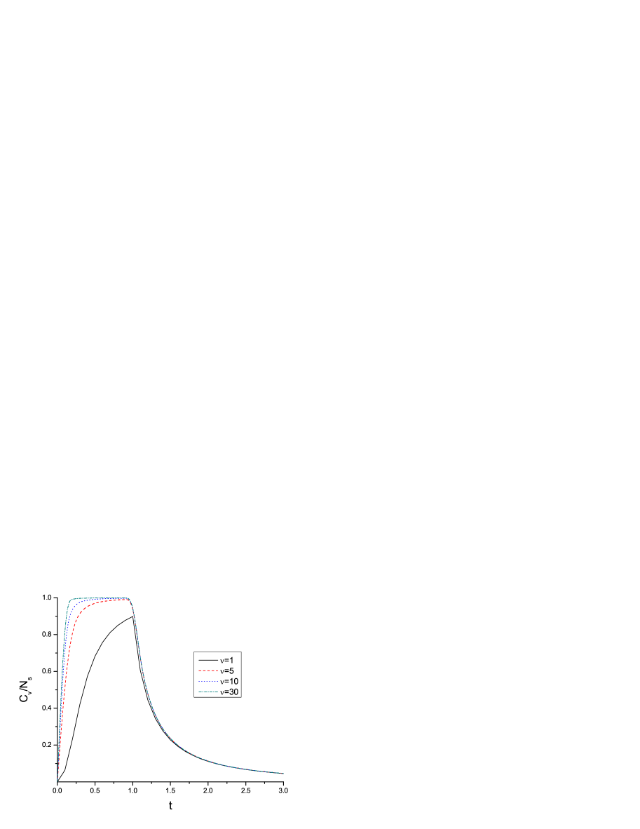
a)

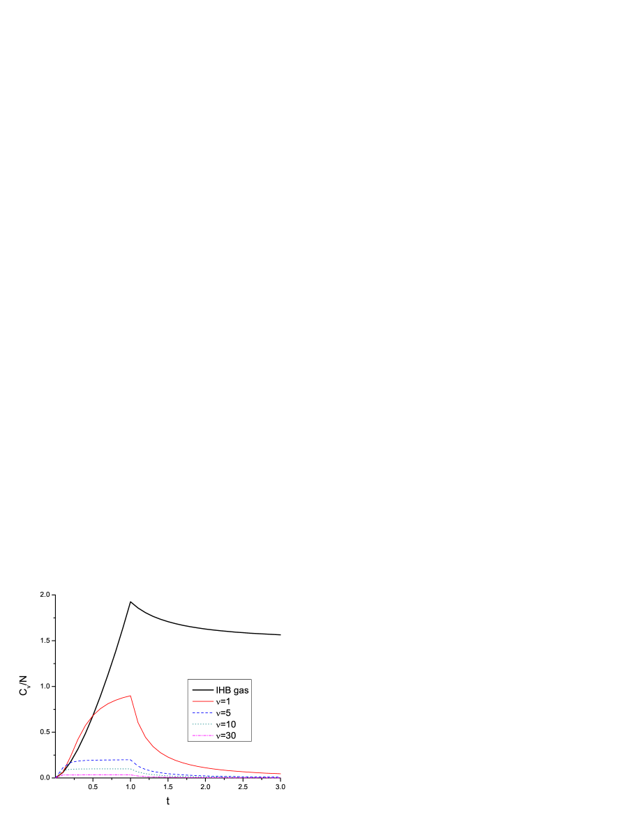
b)

Figure 6: (Color online) The specific heat per site (a), evaluated from Eq. (15), and per particle (b) for different values of $\nu$. The thick solid line in (b) corresponds to the ideal homogeneous Bose gas given by (A.11). The boundary between BEC and normal phases is at $t=1$.

The similar quantities, namely, $\partial C_{v}/\partial T$ per site and per particle for noninteracting Bose gases in optical lattices are presented in figures Fig.7(a) and Fig.7(b) respectively. It is seen that the derivative is discontinuous in this case also. Below we will show how this jump can be evaluated. First we note that the jump in IHB gas presented in Eqs. (6) and (A.14) as

$$\small{\tilde{\Delta}}=\displaystyle\frac{9g_{3/2}(1)}{4g_{1/2}(1)}+\displaystyle\frac{27g_{3/2}^{2}(1)g_{-1/2}(1)}{8g_{1/2}^{3}(1)}$$ (42)

is mainly determined by the singularities of Bose functions near $z=1$ which may be isolated by using Robinson formula robinson

$$\small g_{\sigma}(z)=\displaystyle\frac{\Gamma(1-\sigma)}{\alpha^{2(1-\sigma)}}+regular\quad terms$$ (43)

where $z=\exp(-\alpha^{2})$, $\sigma<1$ , as it was outlined in Appendix A. So, the first term in (42) vanishes, while the second term gives a finite value $\tilde{\Delta}=3.66$.

For ideal optical lattices from equations (16) and (17) one obtains

$$\small\begin{array}[]{l}\nu{\Delta}(\nu)=\displaystyle\frac{{{T_{c}^{0}}}}{N_{s}}\left[\left(\displaystyle\frac{\partial{C}_{v}}{\partial T}\right)_{{T_{c}^{0}}^{-}}-\left(\displaystyle\frac{\partial{C}_{v}}{\partial T}\right)_{{T_{c}^{0}}^{+}}\right]=\displaystyle\frac{R_{112}(1)[6R_{223}(1)-2R_{112}(1)-3R_{212}(1)]}{R_{012}(1)}+\\ \\ \displaystyle\frac{2R_{112}^{2}(1)[R_{112}(1)-3R_{123}(1)]}{R_{012}^{2}(1)}+2R_{112}^{3}(1)\left[\displaystyle\frac{R_{023}(1)}{R_{012}^{3}(1)}\right]\end{array}$$ (44)

As it was shown in the Appendix B, $R_{ijk}(z)|_{z\rightarrow 1}\rightarrow\infty$ due to the infrared divergency for $i-k+1<0.$ Thus in Eq. (44), where the relation in square brackets is evaluated in the Appendix B, only the last term survives. So, using Eq. (B.7) we get following expression

$$\small\nu\Delta(\nu)=32\pi^{2}\left[\displaystyle\frac{R_{112}(1)J}{{T_{c}^{0}}}\right]^{3}.$$ (45)

At first glance it seems that this function behaves like $1/\nu^{3}$ due to the Eq. (19) . However, taking into account the $\nu$ dependence of $R_{112}(1)$ it can be shown that $\nu\Delta(\nu)\sim const$. In fact, especially, for large $\nu$, $(\nu\geq 5)$ using the estimation for $R_{112}(1)$ given in (B.9) one may conclude that $\nu\Delta(\nu)$ does not practically depend on the filling factor, since in this case ${T_{c}^{0}}$ in eq. (45) is cancelled:

$$\small\nu\Delta(\nu)\approx 32\pi^{2}\left[\displaystyle\frac{{T_{c}^{0}}J}{4{T_{c}^{0}}J}\right]^{3}=4.9348$$ (46)

Actually, performing exact numerical calculations using (44) show following values: $\nu\Delta(\nu)\mid_{\nu=1}=3.96$, $\nu\Delta(\nu)\mid_{\nu=5}=4.618$, $\nu\Delta(\nu)\mid_{\nu=10}=4.657$ and $\nu\Delta(\nu)\mid_{\nu=30}=4.661$ (see also Fig. 7(a)). Hence one may conclude that the jump in the heat capacity per particle linearly decreases with increasing the filling factor i.e $\Delta\sim 1/\nu$ as it can be also seen from Fig. 7(b). This is in contrast to the case of IHB gases where the similar quantity does not depend on the density being a constant.

There is one more difference between the $\partial C_{v}/\partial T$ of these two kinds of gases. As it is seen from Figs. 7 it reaches its maximum exactly at the critical temperature for IHB gases, while in the case of optical lattices the maximum is shifted towards smaller values of temperature, $T_{max}<{T_{c}^{0}}$. Moreover, as it is seen from Fig.7a, $T_{c}^{0}(\partial C_{v}/\partial T)/N_{s}$ is insensitive to $\nu$ in the normal phase. These facts may be checked experimentally ruddell by decreasing the interaction between the atoms with a Feshbach resonance technique.

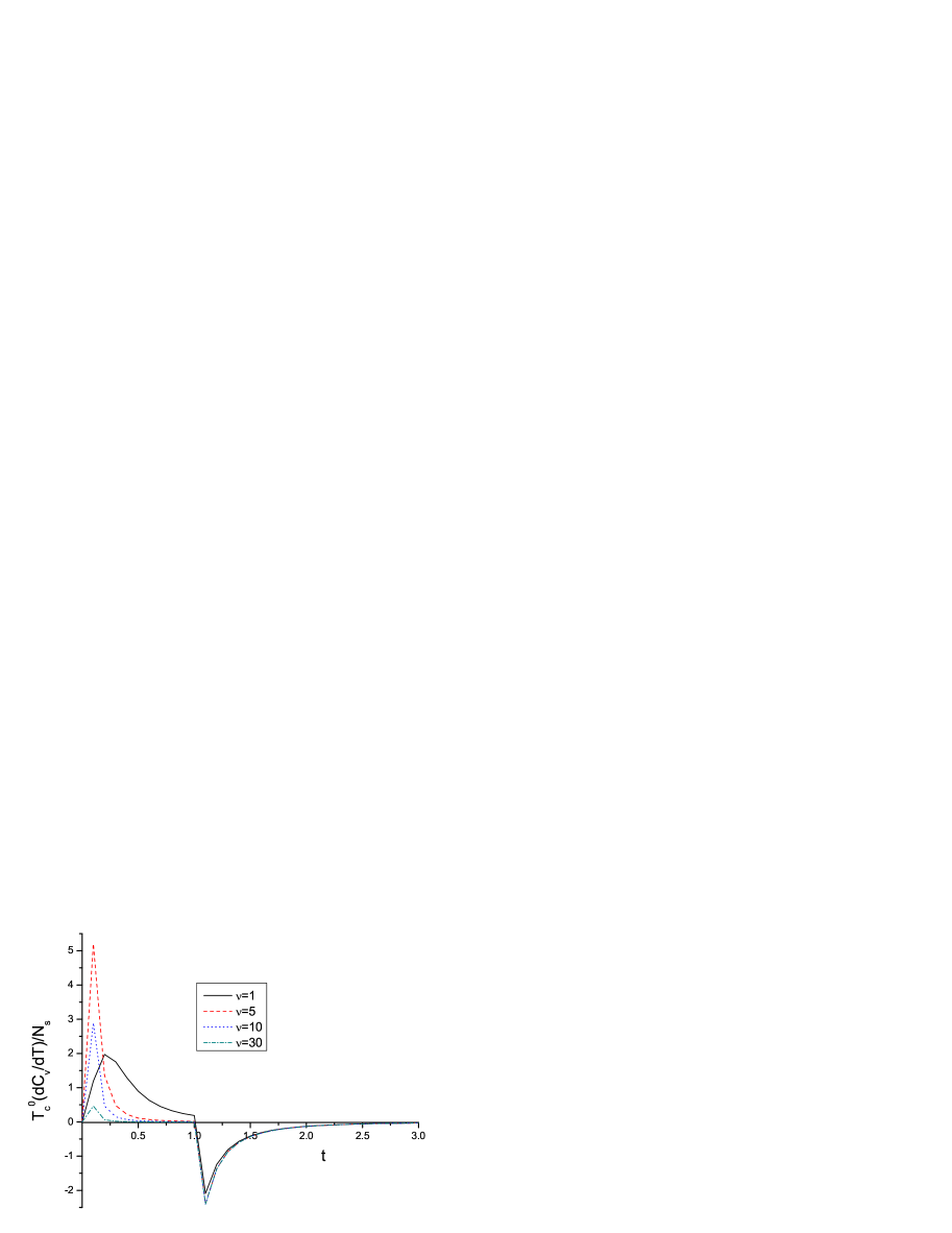
a)

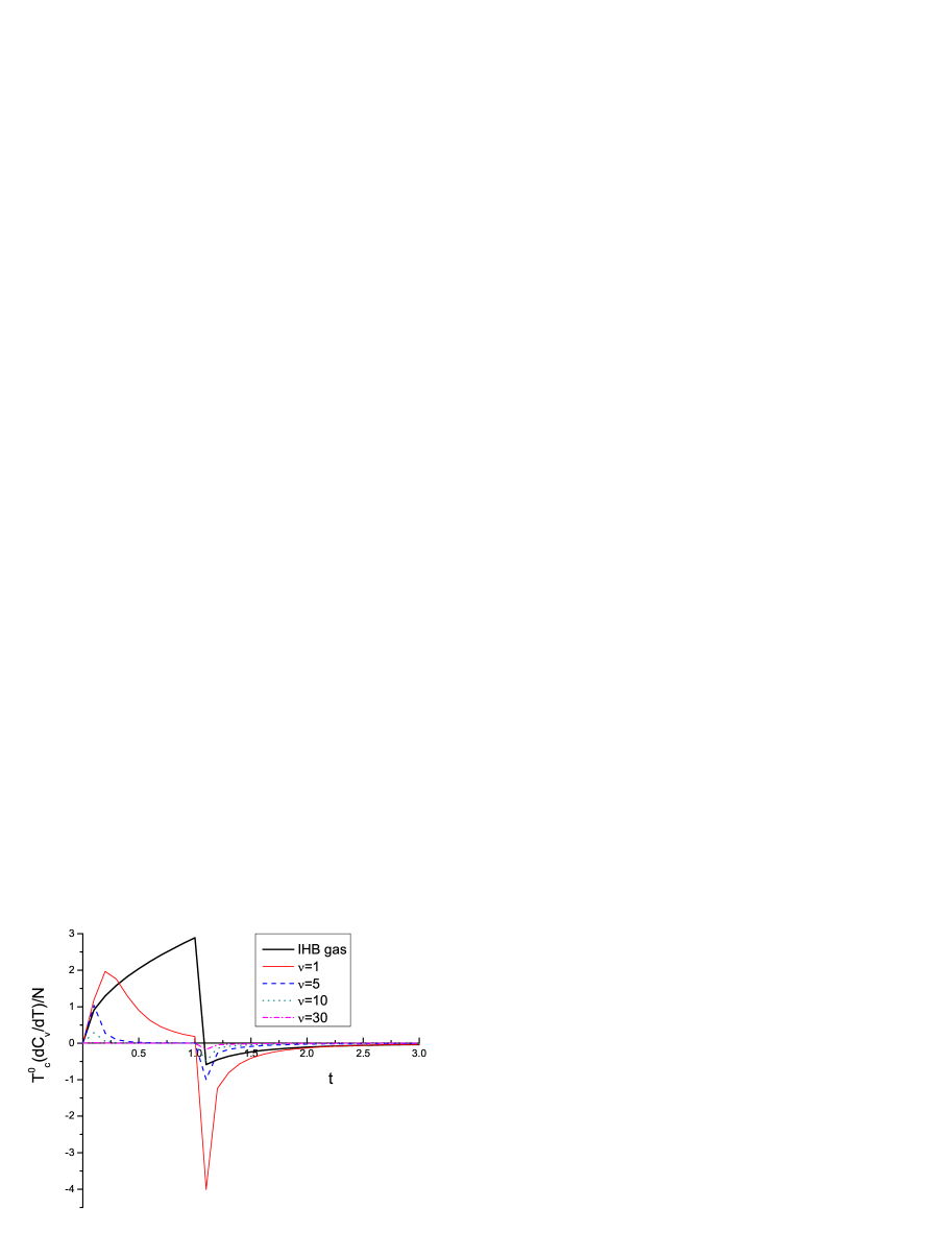
b)

Figure 7: (Color online) The temperature derivative of the specific heat per site (a) and per particle (b) multiplied by factor ${T_{c}^{0}}$ vs reduced temperature t for different values of $\nu$. It is seen that this quantity for the optical lattices does not reach its maximum at $t=1$, even at $\nu=1$ (thin solid lines), in contrast to the ideal homogeneous gas, presented as a thick solid line in (b) (see Eq.s (A.13)).

.

VII Condensate fluctuations in the thermodynamic limit

Number-of-particle fluctuations define the stability of the system and its way of reaching the state of thermodynamic equilibrium fluc1 ; fluc2 . For IHB gases they have been thoroughly studied by Yukalov in Refs. yukpre ; yuklas . Here we outline the main ideas of these works and then discuss the case of noninteracting gases in cubic optical lattices.

The number-of-particle fluctuations are characterized by the dispersion

$$\small\Delta_{f}^{2}=\langle{\hat{N}^{2}}\rangle-\langle{\hat{N}}\rangle^{2}$$ (47)

where ${\hat{N}}$ is the number - of - particle operator. This dispersion is directly related to the isothermal compressibility defined by

$$\small\kappa_{T}\equiv\displaystyle\frac{1}{B}=-\displaystyle\frac{1}{V}\left(\displaystyle\frac{\partial V}{\partial P}\right)_{TN}=\displaystyle\frac{1}{\rho^{2}}\left(\displaystyle\frac{\partial\rho}{\partial\mu}\right)_{TN},$$ (48)

where $B$ is a bulk module, by following equality yukkniga

$$\small\kappa_{T}=\displaystyle\frac{\Delta_{f}^{2}}{TN\rho}$$ (49)

A necessary condition for a system to be stable is the semi-positiveness and finiteness of the compressibility, that is, $0\leq\kappa_{T}<\infty$. If the compressibility (48) were infinite, this would mean that an infinitesimal fluctuation of pressure $P$ would lead to an immediate collapse or explosion of the system. Therefore, in the thermodynamic limit, the dispersion (47) should behave as

$$\small\Delta_{f}^{2}\simeq const\cdot N\quad\quad(N\rightarrow\infty)$$ (50)

When the stability condition (50) is satisfied, the number of particle fluctuations are called normal, but when Eq. (50) is not valid, so that the compressibility (49) diverges in the thermodynamic limit, the fluctuations are termed anomalous.

Now following work yukpre it is easy to show that the ideal homogeneous Bose gas, below the condensation temperature, as an unstable system with anomalous condensate fluctuations. In fact, as it was shown in the Appendix A, the compressibility of IHB gas is given by

$$\small\tilde{\kappa}_{T}=\displaystyle\frac{g_{1/2}(\tilde{z})}{\lambda_{T}^{3}T\tilde{\rho}^{2}}\quad.$$ (51)

In the BEC phase the fugacity equals to unity, $\tilde{z}(T\leq\tilde{T_{c}^{0}})=1$, and hence, due to the divergence of Bose function $g_{1/2}(1)$ the compressibility goes to infinity , $\tilde{\kappa}_{T}\rightarrow\infty$.

On the other hand it was shown many years ago by Politzer politzer that a magnetic trap stabilizes the system of noninteracting bosons whose dispersion became proportional to the number of particles:

$$\small\Delta_{f}^{2}(mag.trap)=1.37N\left(\displaystyle\frac{T}{{T_{c}^{0}}}\right)^{3}$$ (52)

The natural question arises, if the optical trap with the periodic potential (1) is also able to make an ideal Bose gas stable?

Actually, in this case the compressibility may be defined similarly to (48) as follows

$$\small\kappa_{T}=\displaystyle\frac{a^{3}}{\nu^{2}}\left(\displaystyle\frac{\partial\nu}{\partial\mu}\right)_{TN}$$ (53)

Representing (9) as

$$\small\nu=\int_{0}^{1}dq_{1}dq_{2}dq_{3}\displaystyle\frac{1}{e^{\beta\varepsilon(q)}z^{-1}-1}$$ (54)

and differentiating this equation with respect to $\mu$ we obtain

$$\small B^{-1}=\kappa_{T}=\displaystyle\frac{a^{3}R_{012}(z)}{zT\nu^{2}}$$ (55)

where $B$ is the bulk module of the noninteracting gas in an optical lattice. From Eqs. (55) and (49) it is immediately understood that in the BEC regime the ideal optical lattice has an infinitely large particle fluctuations, i.e. $(\Delta_{f}^{2}/N)(BEC)\rightarrow\infty$ and hence becomes unstable, since $\displaystyle\lim_{\mu\rightarrow 0}R_{012}(z(\mu))=\infty$ (see Appendix B). This is in good agreement with experimental observations. For instance, Roati et al. roatiprl have shown that the lifetime of the BEC in the optical trap, which is typically around 3 s, is significantly shortened when $a_{s}$ is extremely decreased.

One more conclusion concerning the scale properties of these two kinds of gases can be made by introducing dimensionless compressibility as $\kappa^{\prime}_{T}={T_{c}^{0}}\kappa_{T}\rho$. For IHB gas this quantity may be represented as $\tilde{\kappa}^{\prime}=\sqrt{t}g_{1/2}(\tilde{z})/g_{3/2}(1)$, as it was shown in the Appendix A. As to the ideal gas in optical lattice the similar quantity is $\kappa^{\prime}_{T}=R_{012}(z)/zt\nu$. Again we conclude that the dimensionless compressibility does not explicitly depend on the density for IHB gases but it does for optical lattices.

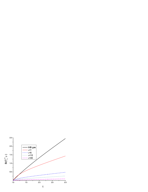
Figure 8: (Color online) The bulk module in units ${T_{c}^{0}}\rho$ vs reduced temperature t for different values of $\nu$. In the BEC phase, when $t\leq 1$ it equals to zero. The thick solid line corresponds to IHB gas (see Eq. (A.16)).

.

In Fig. 8 the dimensionless bulk module, as an inverse of $\kappa^{\prime}_{T}$, is presented for IHB gas as well as for ideal optical lattice. It is seen that in the normal phase the module , and hence the compressibility is positive and finite. Thus we may complete this section with following conclusion : Both kinds of gases under the consideration are unstable in the BEC phase but stable in the normal phase .

VIII conclusion

We have studied thermodynamic properties of ideal gases loaded into the cubic periodic lattice potential in $d=3$ without a harmonic trap for arbitrary integer filling factors and compared them with that of ideal homogeneous Bose gases. Although in real experiments a harmonic confinement is always present, we hope that our results obtained for the homogenious case may represent a suitable starting point for addressing the trapped problem within a Thomas-Fermi approximation.

It have been shown by exact numerical calculations that in contrast to the case of an IHB gas, the energy as well as the entropy of ideal optical lattice exhibits a linear dependence on temperature in the BEC phase and becomes almost a constant in the normal phase for large filling factors. We have evaluated the jump in $dC_{v}/dT$ and shown that jump in the heat capacity per particle linearly decreases with increasing the filling factor i.e. $\Delta\sim 1/\nu$. It is interesting to note that $dC_{v}/dT$ for an ideal optical lattice reaches its maximum not at the critical temperature, as it does for IHB gas, but at rather smaller temperature.

We have shown that scaling properties of these two kinds of gases are different. For example the thermodynamic potential of IHB gas in units of the critical temperature may be presented as an explicit function of only the reduced temperature as $\Omega/{T_{c}^{0}}\sim\Omega^{\prime}(t)$, while that of the ideal optical lattice may be not. Moreover, the well known relation $E=-d\Omega/2$ between the energy and the thermodynamic potential does not hold for the ideal gas in the periodic potential.

Studying the bulk properties of an ideal gas in the thermodynamic limit have shown that both kind of gases are unstable below the critical temperature . So it seems impossible to create a stable ideal gas of atoms even with Feshbach resonance technique. For this reason any calculation concerning an ideal gas should be considered as a model one. Nevertheless, such calculations are useful. For example they have already been used to estimate the shift of critical temperature $\Delta T_{c}=(T_{c}-T_{c}^{0})$ of real gases due to the interaction and finite size effects blakiepra76 , or a disorder potential lopatin . For real gases at high filling region $\Delta T_{c}$ may be estimated by using $1/\nu$ expansion fischer or effective potential methods teichmann ; axel

The present work will give an opportunity for the estimations in future experiments and QMC calculations for large values of $\nu$ and may serve as a check point in theoretical studies in the limit $(U/J)\rightarrow 0$.

Appendix A

Here we bring a summary of main explicit formulas for ideal homogeneous Bose gases . The most of them can be directly derived from eq. (8) by using well known thermodynamic relations landau ; huang .

• The density:

  $$\small\rho=\displaystyle\frac{N}{V}=\sum_{k}\displaystyle\frac{1}{z^{-1}e^{\beta\varepsilon(k)}-1}=\displaystyle\frac{g_{3/2}(z)}{\lambda_{T}^{3}}$$ (A.1)

  where $\sum_{k}f(k)=V\displaystyle\int d{\bf k}f(k)/(2\pi)^{3}$, $\varepsilon(k)={\bf k}^{2}/2m$, $\lambda_{T}=\sqrt{2\pi/Tm}$ and robinson

  $$\small\begin{array}[]{l}g_{\sigma}(z)=\displaystyle\frac{1}{\Gamma(\sigma)}\int_{0}^{\infty}\displaystyle\frac{x^{(\sigma-1)}dx}{\exp(x)z^{-1}-1}=\Gamma(1-\sigma){\tilde{\alpha}}^{\sigma-1}+\displaystyle\sum_{l=0}^{\infty}\displaystyle\frac{(-1)^{l}}{l!}\zeta(\sigma-l){\tilde{\alpha}}^{l}\quad,\\ {\tilde{\alpha}}=-\beta\mu=-\ln z\end{array}$$ (A.2)

  is the Bose function satisfying the recurrency formula

  $$\small\displaystyle\frac{\partial g_{\sigma}(z)}{\partial z}=\displaystyle\frac{g_{\sigma-1}(z)}{z}$$ (A.3)

• The condensed fraction:

  $$\small n_{0}=1-t^{3/2}$$ (A.4)

  where $t=T/{\tilde{T}}_{c}^{0}$ is the reduced temperature.

• The critical temperature is defined from eq. (A.1) at $z=1$ as:

  $$\small{\tilde{T}_{c}^{0}}=\displaystyle\frac{1.05\pi}{m}\rho^{2/3}.$$ (A.5)

  Here and below we use numerical values of Bose functions such as $g_{3/2}(1)=2.6124$, $g_{5/2}(1)=1.3415$ etc.

• The thermodynamic potential and pressure. Integration by parts in equation (8) gives

  $$\small\displaystyle\frac{\Omega}{N{\tilde{T}_{c}^{0}}}=-\displaystyle\frac{PV}{N{\tilde{T}_{c}^{0}}}=-\displaystyle\frac{Vm^{3/2}\sqrt{2}T^{5/2}g_{5/2}(z)}{4\pi^{3/2}{N{\tilde{T}_{c}^{0}}}}\\ \\ =\left\{\begin{array}[]{ll}-0.513t^{5/2}&(T\leq{\tilde{T}_{c}^{0}})\\ -0.383t^{5/2}g_{5/2}(z)&(T>{\tilde{T}_{c}^{0}})\end{array}\right.$$ (A.6)

• The fugacity. Clearly, in the BEC phase $z=\exp(\mu/T)$ equals to unity i.e. $z(T\leq{T_{c}^{0}})=1$. In the normal phase it can be evaluated as a solution to the equation (A.1) with a given density $\rho$ and temperature. Near the critical temperature, when $\mu<<T$ we may use Robinsons formula Eq. (A.2) and solve (A.1) analytically to find following approximation in the normal phase

  $$\small{\tilde{z}}\approx\exp(-0.54+1.1/t^{3/2}-0.54/t^{3})\leq 1\quad if\quad t>1$$ (A.7)

  Its temperature derivative $z^{\prime}=\partial z/\partial T$ can be found by differentiation the both sides of eq. (A.1) with the fixed $\rho$ with respect to $T$ , i.e. the equation $d\rho/dT=0$. As a result one obtains

  $$\small z^{\prime}{\tilde{T}_{c}^{0}}=\left\{\begin{array}[]{ll}0&(T\leq{\tilde{T}_{c}^{0}})\\ -\displaystyle\frac{3zg_{3/2}(z)}{2tg_{1/2}(z)}&(T>{\tilde{T}_{c}^{0}})\end{array}\right.$$ (A.8)

• Entropy and energy.

  $$\small\displaystyle\frac{S}{N}=\displaystyle\frac{5m^{3/2}\sqrt{2}T^{3/2}g_{5/2}(z)}{8\pi^{3/2}\rho}\\ \\ =\left\{\begin{array}[]{ll}1.283t^{3/2}&(T\leq{\tilde{T}_{c}^{0}})\\ 0.957t^{3/2}g_{5/2}(z)&(T>{\tilde{T}_{c}^{0}})\end{array}\right.$$ (A.9)

  The energy per particle, when the zero temperature energy is subtracted is given by

  $$\small\displaystyle\frac{E}{N}=\left\{\begin{array}[]{ll}0.77{\tilde{T}_{c}^{0}}t^{5/2}&(T\leq{\tilde{T}_{c}^{0}})\\ 0.574{\tilde{T}_{c}^{0}}t^{5/2}g_{5/2}(z)&(T>{\tilde{T}_{c}^{0}})\end{array}\right.$$ (A.10)

• The heat capacity and its slope. The exact expression for the heat capacity per particle $C_{v}/N$, given in textbooks,

  $$\small\begin{array}[]{l}\displaystyle\frac{C_{v}}{N}=\left\{\begin{array}[]{ll}\displaystyle\frac{15\zeta(5/2)}{4\zeta(3/2)}t^{3/2}&(T\leq{\tilde{T}_{c}^{0}})\\ \\ \displaystyle\frac{15g_{5/2}(z)}{4g_{3/2}(z)}-\displaystyle\frac{9g_{3/2}(z)}{4g_{1/2}(z)}&(T>{\tilde{T}_{c}^{0}})\end{array}\right.\end{array}$$ (A.11)

  where $\zeta(x)$ is the Riemann function, may be repalced by a nice and more practical approximation given in ref. wang

  $$\small\begin{array}[]{l}\displaystyle\frac{C_{v}}{N}=\left\{\begin{array}[]{ll}1.926t^{3/2}&(T\leq{\tilde{T}_{c}^{0}})\\ \\ 1.496+0.341t^{-3/2}+0.089t^{-3}&(T>{\tilde{T}_{c}^{0}})\end{array}\right.\end{array}$$ (A.12)

  Differentiating the last equation one obtains

  $$\small\begin{array}[]{l}\displaystyle\frac{{\tilde{T}_{c}}}{N}\left(\displaystyle\frac{\partial C_{v}}{\partial T}\right)_{V}=\left\{\begin{array}[]{ll}2.899t^{1/2}&(T\leq{\tilde{T}_{c}^{0}})\\ \\ -0.511t^{-5/2}-0.267t^{-4}&(T>{\tilde{T}_{c}^{0}})\end{array}\right.\end{array}$$ (A.13)

  The discontinuity in the slope of the heat capacity may be evaluated directly from the equation (A.13) as

  $$\small\begin{array}[]{l}{\tilde{\Delta}}=\displaystyle\frac{{\tilde{T}_{c}}}{N}\left[\left(\displaystyle\frac{\partial{\tilde{C}}_{v}}{\partial T}\right)_{\tilde{T}_{c}^{-}}-\left(\displaystyle\frac{\partial{\tilde{C}}_{v}}{\partial T}\right)_{\tilde{T}_{c}^{+}}\right]=\displaystyle\frac{9g_{3/2}(1)}{4g_{1/2}(1)}+\displaystyle\frac{27g_{3/2}^{2}(1)g_{-1/2}(1)}{8g_{1/2}^{3}(1)}=\\ \\ \left[2.889t^{1/2}+0.511t^{-5/2}+0.267t^{-4}\right]_{t\rightarrow 1}=0.36675\end{array}$$ (A.14)

• The compressibility. Being defined as

  $$\small\kappa_{T}=\displaystyle\frac{1}{\rho^{2}}\left(\displaystyle\frac{\partial\rho}{\partial\mu}\right)_{N,T}$$ (A.15)

  the compressibility $\kappa_{T}$ can be directly obtained from (A.1) . The result is

  $$\small\begin{array}[]{l}\kappa_{T}\rho\tilde{T}_{c}^{0}=\left\{\begin{array}[]{ll}\infty&(T\leq{\tilde{T}_{c}^{0}})\\ \\ 0.3828{\sqrt{t}g_{1/2}(z)}&(T>{\tilde{T}_{c}^{0}})\end{array}\right.\end{array}$$ (A.16)

  Note that the bulk module is defined as $B=1/\kappa_{T}$.

Appendix B

Here we consider the functions $R_{ijk}(z)$ defined as

$$\small\begin{array}[]{l}R_{ijk}(z)=\int_{0}^{1}dq_{1}dq_{2}dq_{3}\displaystyle\frac{x^{i}e^{jx}}{\left[e^{x}z^{-1}-1\right]^{k}},\\ x=\beta\varepsilon(q)\end{array}$$ (B.1)

For IHB gases the similar functions are Bose functions whose expansion was given by Robinson robinson as in the Eq. (A.2). From (A.2) it is seen that in the BEC regime for ideal gas, when $\mu\rightarrow 0$ and $\sigma<1$, $g_{\sigma}({\tilde{\alpha}})$ diverges, e.g. $g_{1/2}({\tilde{\alpha}})\sim\sqrt{\pi}/\sqrt{{\tilde{\alpha}}}$.

Similarly it is easy to understand that when the chemical potential goes to zero the function in (B.1) goes to infinity, i.e. $R_{ijk}(z)|_{z\rightarrow 1}\rightarrow\infty$ due to the infrared divergency for $i-k+1<0$ and is regular otherwise. Below we show how this divergency can be isolated and presented analytically e.g. for $R_{012}(z)$ and $R_{023}(z)$. To do this we use Debye like approximation ourknr1 ; Yukalovobsor :

$$\small\begin{array}[]{l}\displaystyle\int_{0}^{1}dq_{1}dq_{2}dq_{3}\rightarrow\displaystyle\frac{\pi}{2}\displaystyle\int_{0}^{q_{d}}q^{2}dq;\\ \varepsilon(q)=2J\varepsilon^{\prime}(q),\quad\quad\varepsilon^{\prime}(q)=\displaystyle\frac{\pi^{2}q^{2}}{2},\quad\quad q_{d}=\left(\displaystyle\frac{6}{\pi}\right)^{1/3}.\\ \end{array}$$ (B.2)

Introducing $T^{\prime}=T/J$, $z=\exp(\mu/T)\equiv\exp(-\alpha^{2})$ and expanding the exponent, we represent $R_{ijk}(z)$ as

$$\small R_{ijk}(z)\mid_{\alpha\rightarrow 0}=\displaystyle\frac{\pi}{2}\displaystyle\int_{0}^{q_{d}}q^{2}dq\displaystyle\frac{x^{i}e^{jx}}{(x+\alpha^{2})^{k}}$$ (B.3)

where $x=\varepsilon(q)\beta=\pi^{2}q^{2}/T^{\prime}$. In particular

$$\small\begin{array}[]{l}R_{012}(z)\mid_{z\rightarrow 1}=\displaystyle\frac{(T^{\prime})^{3/2}}{2\pi^{2}}\displaystyle\int_{0}^{y_{d}}y^{2}dy\displaystyle\frac{1+y^{2}}{(y^{2}+\alpha^{2})^{2}}\\ \\ R_{023}(z)\mid_{z\rightarrow 1}=\displaystyle\frac{(T^{\prime})^{3/2}}{2\pi^{2}}\displaystyle\int_{0}^{y_{d}}y^{2}dy\displaystyle\frac{1+2y^{2}}{(y^{2}+\alpha^{2})^{3}}\\ \\ R_{001}(z)\mid_{z\rightarrow 1}=\displaystyle\frac{(T^{\prime})^{3/2}}{2\pi^{2}}\displaystyle\int_{0}^{y_{d}}dy\displaystyle\frac{y^{2}}{(y^{2}+\alpha^{2})}\\ \end{array}$$ (B.4)

where $y_{d}=\pi q_{d}/\sqrt{T^{\prime}}$. The explicit integration gives

$$\small\begin{array}[]{l}R_{012}(z)\mid_{z\rightarrow 1}=\displaystyle\frac{(T^{\prime})^{3/2}}{4\pi^{2}}\left[\displaystyle\frac{y_{d}(2y_{d}^{2}+3\alpha^{2}-1)}{y_{d}^{2}+\alpha^{2}}-\displaystyle\frac{(3\alpha^{2}-1)\arctan(y_{d}/\alpha)}{\alpha}\right]\\ \\ R_{023}(z)\mid_{z\rightarrow 1}=\displaystyle\frac{(T^{\prime})^{3/2}}{16\pi^{2}}\left[\displaystyle\frac{y_{d}(-\alpha^{2}-6\alpha^{4}+y_{d}^{2}-10y_{d}^{2}\alpha^{2})}{\alpha^{2}(y_{d}^{2}+\alpha^{2})^{2}}+\displaystyle\frac{(6\alpha^{2}+1)\arctan(y_{d}/\alpha)}{\alpha^{3}}\right]\\ \\ R_{001}(z)\mid_{z\rightarrow 1}=\displaystyle\frac{(T^{\prime})^{3/2}}{2\pi^{2}}\left[y_{d}-{\alpha\arctan(y_{d}/\alpha)}\right]\\ \end{array}$$ (B.5)

Now expanding in powers of $\alpha$ one obtains

$$\small\begin{array}[]{l}R_{012}(z)=\displaystyle\frac{(T^{\prime})^{3/2}}{8\pi\alpha}+regular\quad terms\\ \\ R_{023}(z)=\displaystyle\frac{(T^{\prime})^{3/2}}{32\pi\alpha^{3}}+\displaystyle\frac{3(T^{\prime})^{3/2}}{16\pi\alpha}+regular\quad terms\\ \\ R_{001}(z)=\displaystyle\frac{T^{\prime}6^{1/3}}{2\pi^{4/3}}-\displaystyle\frac{(T^{\prime})^{3/2}\alpha}{4\pi}+\displaystyle\frac{(T^{\prime})^{2}6^{2/3}\alpha^{2}}{12\pi^{8/3}}+O(\alpha^{3})\end{array}$$ (B.6)

where the regular terms are finite at $\alpha\rightarrow 0$ and may be calculated more accurately by the exact three dimensional integration. As to $R_{001}(z)$ which will be used below to study the fugacity $z=\exp(-\mid\mu\mid/T)$ near ${T_{c}^{0}}$, it is regular at small $\mid\mu\mid/T\equiv\alpha^{2}$, as expected.

Now we are on the stage of calculating the relation $\displaystyle\lim_{z\rightarrow 1}R_{023}(z)/R_{012}^{3}(z)$ which is necessary to evaluate the jump in the heat capacity. From equation (B.6) one immediately obtains

$$\small\lim_{z\rightarrow 1}\displaystyle\frac{R_{023}(z)}{R_{012}^{3}(z)}=16\pi^{2}\left[\displaystyle\frac{J}{{T_{c}^{0}}}\right]^{3}$$ (B.7)

.

For completeness we estimate also $R_{112}(1)$ which is used to evaluate the discontinuity in the slope of the specific heat in eq. (44). In fact, for large $\nu$, $(\nu\geq 5)$ one may represent $R_{112}(1)$ as

$$\small\begin{array}[]{l}R_{112}(1)=\displaystyle\int_{0}^{1}dq_{1}dq_{2}dq_{3}\displaystyle\frac{\varepsilon(q)\beta e^{\varepsilon(q)\beta}}{\left[e^{\varepsilon(q)\beta}z^{-1}-1\right]^{2}}\approx{T_{c}^{0}}\displaystyle\int_{0}^{1}\displaystyle\frac{dq_{1}dq_{2}dq_{3}}{\varepsilon(q)}=\displaystyle\frac{{T_{c}^{0}}}{2J}\displaystyle\int_{0}^{1}\displaystyle\frac{dq_{1}dq_{2}dq_{3}}{\tilde{\varepsilon}(q)}\end{array}$$ (B.8)

where $\tilde{\varepsilon}(q)=\displaystyle\sum_{\alpha=1}^{3}(1-\cos\pi q_{\alpha})$ Now evaluating the last integral numerically gives following final expression :

$$\small R_{112}(1)\approx\displaystyle\frac{{T_{c}^{0}}}{4J}$$ (B.9)

Similarly to IHB gas one may obtain an approximation for the fugacity of an ideal optical lattice, starting from following equation

$$\small\nu=\displaystyle\int_{0}^{1}\displaystyle\frac{dq_{1}dq_{2}dq_{3}}{z^{-1}e^{\beta\varepsilon(q)}-1}\equiv R_{001}(z)$$ (B.10)

Near the critical temperature, $\alpha$, defined through $\alpha^{2}=-\ln(z)=\mid\mu\mid/T$, is small, so one may use Robinson like expansion (B.6) for $R_{001}(z)$ to solve (B.10) analytically. As a result we obtain

$$\small\begin{array}[]{l}\alpha\approx\displaystyle\frac{2(6/\pi)^{1/3}}{(C_{\nu}t\nu)^{1/2}}-\displaystyle\frac{4\pi\nu}{(C_{\nu}t\nu)^{3/2}}\quad,\quad z=\exp(-\alpha^{2})\end{array}$$ (B.11)

where $C_{\nu}=3.96\exp(0.37/\nu)$ and $T$ is presented as $T=t{T_{c}^{0}}$, with ${T_{c}^{0}}$ given by (19). From this equations as well as from Fig.(4)(c) one may conclude that the fugacity goes to unity with the increasing of the filling factor $\nu$. As to $z^{\prime}=dz/dT$ defined in equation (13) it is clear that $z^{\prime}(T)\mid_{T=T_{c}^{0+}}=0$. Thus, near ${T_{c}^{0}}$ both $z$ and $z^{\prime}$ are continuous.

References

- (1) E. Timmermans, P. Tomassini, M. Hussein and A. Kerman, Phys. Rep. 315 (1999) 199.
- (2) G. Roati et al. Phys. Rev. Lett. 99(2007) 010403.
- (3) G. Roati et al. Nature 453(2007)895.
- (4) Y. Shin et al., Phys. Rev. Lett. 92(2004)050405.
- (5) L. Pezzé et al., Phys. Rev. A72(2005) 043612.
- (6) D. Baillie and P. B. Blakie, Phys. Rev. A80(2009) 031603(R) .
- (7) D. Baillie and P. B. Blakie, Phys. Rev. A80(2009) 033620.
- (8) M. Lewenstein, A. Sanpera, and V. Ahufinger, Ultracold atoms in optical lattices: Simulating quantum many-body systems ,Oxford University Press, Oxford, 2012.
- (9) N. R. Cooper, Phys. Rev. Lett.,106 (2011) 175301 .
- (10) W. Zwerger, J. Opt. B5 (2003)S9
- (11) H.T.C. Stoof, K.B. Gubbels, and D.B.M. Dickerscheid, Ultracold Quantum Fields ,Springer, Berlin, 2009.
-
(12)
V. I. Yukalov, Laser Physics 19(2009)1 ;
V. I. Yukalov, Condensed Matter Physics, 16(2013) 23002. - (13) L. D. Landau and E. M. Lifshitz, E. M. Statistical Physics, Part 1 Oxford, England: Pergamon Press, 1980
- (14) Kerson Huang, Introduction to Statistical Physics Second Edition, CRC Press, 2001.
- (15) Frank Y.-H. Wang, Am. J. Phys. 72(2004)1193
- (16) F. Mancarella, G. Mussardo and A. Trombettoni, Nucl. Phys. B887 (2014) 216 .
- (17) A. Rakhimov, S. Mardonov, E.Ya. Sherman, Ann. Phys. 326(2011) 2499 .
- (18) M. Matsumoto, B. Normand, T. M. Rice, and M. Sigrist, Phys. Rev. B69(2004) 054423 .
- (19) W. Li, A.K. Tuchman, H.C. Chien and M.A. Kasevich, Phys. Rev. Lett. 98 (2007) 040402.
- (20) I. Danshita, A. Polkovnikov, Phys. Rev. A 84 (2011) 063637.
- (21) Z. Hadzibabic , S. Stock , B. Battelier ,V. Bretin , J. Dalibard, Phys. Rev. Lett. 93 (2004) 180403.
- (22) S. Foelling, A. Widera, T. Mueller, F. Gerbier, I. Bloch Phys. Rev. Lett. 97 (2006) 060403.
- (23) H.Kleinert, Z. Narzikulov, A. Rakhimov, Journal of Statistical Mechanics: Theory and Experiment Vol. 2014,(2014) P01003 .
- (24) H. Kleinert, Z. Narzikulov, A. Rakhimov Phys. Rev. A85(2012) 063602 .
- (25) R. K. Pathria, Statistical Mechanics, 2nd ed. Butterworth-Heinemann, Boston, 1996.
- (26) A. Rakhimov and I. N. Askerzade, Phys. Rev. E90(2014) 032124.
- (27) W. Ketterle and N. J. van Druten, Phys. Rev. A54(1996)656.
- (28) P. B. Blakie and J. V. Porto, Phys. Rev. A69(2004)013603.
- (29) R. Ramakumar and A. N. Das, Phys. Lett. A348 (2006)304.
- (30) J. E. Robinson Phys. Rev. 83 (1951) 678.
- (31) S. K. Ruddell, D. H. White, A. Ullah, M. D. Hoogerland, arXiv:1409.5494 (2014)
- (32) D.J. Evans and D.J. Searles, Adv. Phys. 51(2002) 1529 .
- (33) R. Dewar, J. Phys. A36, (2003)631 .
- (34) V. I. Yukalov Phys. Rev. E72(2005)066119 .
- (35) V. I. Yukalov Laser Phys. Lett. 1 (2004) 435 .
- (36) V. I. Yukalov, Statistical Green’s Functions, Queen’s University, Kingston, 1998.
- (37) H. D. Politzer, Phys. Rev. A54 (1996)5048.
- (38) P. B. Blakie1, and Wen-Xin Wang, Phys. Rev. A76 (2007) 053620.
- (39) A.V. Lopatin and V. M. Vinokur, Phys. Rev. Lett. 88 (2002) 235503.
- (40) Uwe R. Fischer, Ralf Schützhold, and Michael Uhlmann, Phys. Rev. A 77, (2008) 043615 .
- (41) N. Teichmann, D. Hinrichs, M. Holthaus, A. Eckardt, Phys. Rev. B 79 (2009) 100503.
- (42) F. E. A. dos Santos and A. Pelster, Phys. Rev. A 79 (2009) 013614.