A Stringy (Holographic) Pomeron with Extrinsic Curvature

Abstract

We model the soft pomeron in QCD using a scalar Polyakov string with extrinsic curvature in the bottom-up approach of holographic QCD. The overall dipole-dipole scattering amplitude in the soft pomeron kinematics is shown to be sensitive to the extrinsic curvature of the string for finite momentum transfer. The characteristics of the diffractive peak in the differential elastic $pp$ scattering are affected by a small extrinsic curvature of the string.

I introduction

The high energy proton on proton (anti-proton) cross sections are dominated by Pomeron exchange, an effective object corresponding to the highest Regge trajectory. The slowly rising cross sections are described by the soft Pomeron with intercept $\alpha_{P}(0)-1\approx 0.08$ and vacuum quantum numbers. Reggeon exchanges have smaller intercepts and are therefore subleading. Reggeon theory for hadron-hadron scattering with large rapidity intervals provide an effective explanation for the transverse growth of the cross sections Gribov et al. (1983).

The transverse growth of the proton with rapidity $\chi$ follows from the BFKL ladders Kuraev et al. (1976); Lipatov (1976); Sterman (1999); Fadin et al. (1975); Balitsky and Lipatov (1978) at weak coupling in QCD. Collinear gluon bremsstrahlung is large even when the coupling is weak and requires re-summation. The ensuing BFKL hard Pomeron carries a large intercept and zero slope. The intercept is slightly improved by higher order perturbative corrections to the BFKL ladder.

The soft Pomeron kinematics suggests an altogether non-perturbative approach. Through duality arguments, Veneziano suggested long ago that the soft Pomeron is a closed string exchange Veneziano (1968). In QCD the closed string world-sheet can be thought as the surface spanned by planar gluon diagrams or fish-nets Greensite (1985). The quantum theory of planar diagrams in supersymmetric gauge theories is tractable in the double limit of a large number of colors $N_{c}$ and ^′ t Hooft coupling $\lambda=g^{2}N_{c}$ using the AdS/CFT holographic approach Maldacena (1998).

In the past decade there have been several attempts at describing the soft pomeron using holographic QCD Rho et al. (1999); Janik and Peschanski (2000); Janik (2001); Polchinski and Strassler (2002, 2003); Brower et al. (2007, 2009, 2010, 2011); Hatta et al. (2008a, b); Albacete et al. (2008, 2009); Basar et al. (2012); Stoffers and Zahed (2013a); Stoffers and Zahed (2012); Stoffers and Zahed (2013b); Qian and Zahed (2012); Shuryak and Zahed (2014). In this letter we follow the work in Stoffers and Zahed (2013a); Stoffers and Zahed (2012); Stoffers and Zahed (2013b) and describe the soft pomeron as an effective string with extrinsic curvature in 5-dimensions. This is inherently a bottom-up approach with the holographic or 5th direction playing the role of the scale dimension for the closed string. The geometry is that of AdS₅ with a wall. In the UV AdS₅ enforces conformality which is a property of QCD-BFKL-kernels, while in the IR the wall enforces confinement a generic feature of QCD.

In section 2 we review the set up for dipole-dipole scattering through a closed string exchange. In section 3, we introduce the QCD effective action with a finite string tension and extrinsic curvature and use it to derive the closed string exchange propagator in flat $5=2+D_{\perp}$ dimensions. In section 4, we detail how the extrinsic curvature modifies the correlation of twisted Wilson loops, and show how it affects the position of the diffractive peak in the differential elastic $pp$ scattering cross section. Our conclusions are in section 5. In the Appendix, we show how the extrinsic curvature affects the stringy interaction between two static dipoles.

II Dipole-Dipole Scattering

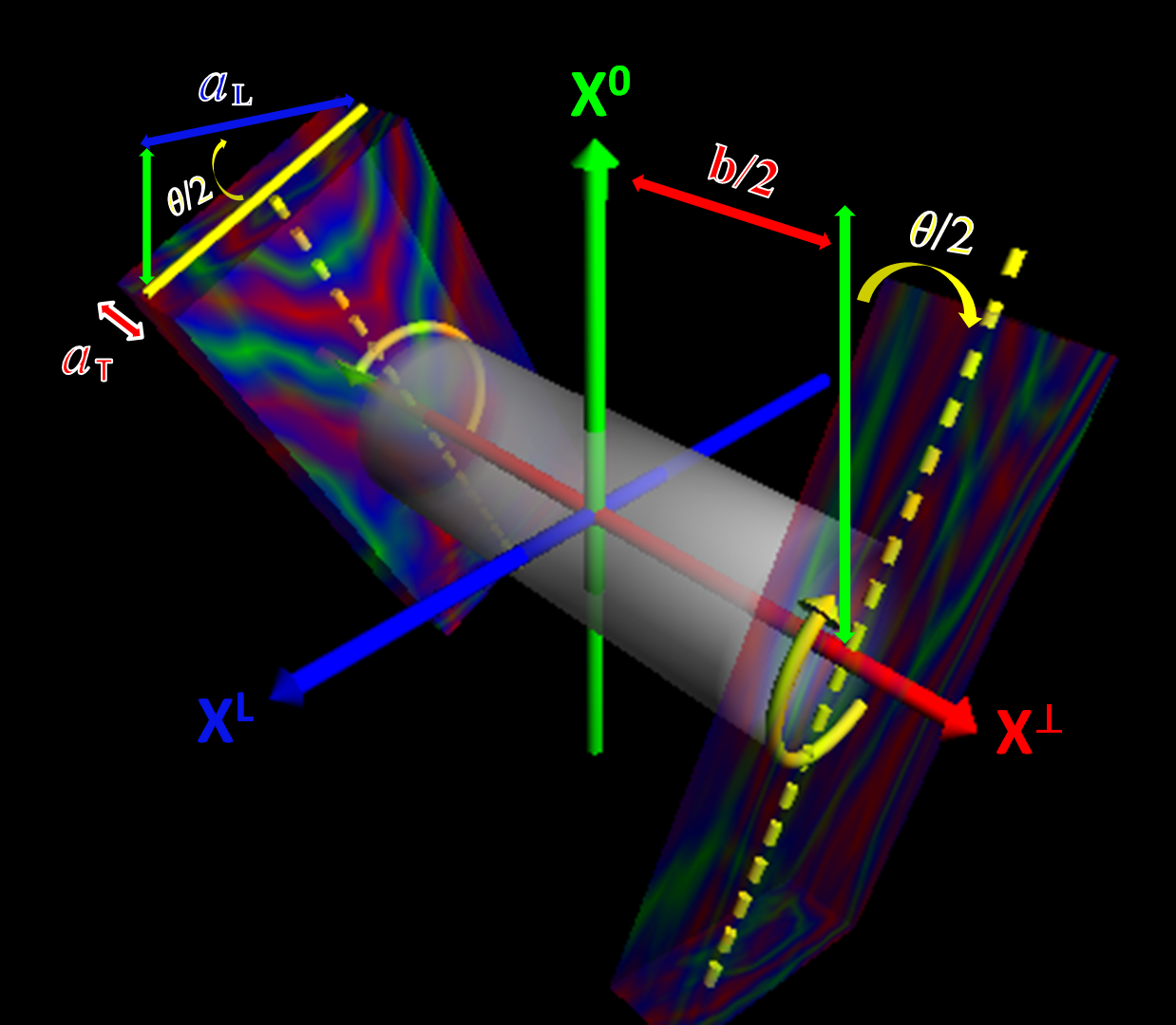
Figure 1: Dipole-Dipole Scattering.

In this section we briefly review the set-up for dipole-dipole scattering using an effective string theory. For that we follow Basar et al. (2012) and consider the elastic scattering of two dipoles

$$D_{1}(p_{1})+D_{2}(p_{2})\rightarrow D_{1}(k_{1})+D_{2}(k_{2})$$ (2.0.1)

as depicted in Fig. 1. $a_{T}$ and $a_{L}$ are the dipoles transverse and longitudinal lengths respectively set near the UV boundary of AdS₅, $b$ is impact parameter and the angle $\theta$ is the Euclidean analogue of the rapidity interval

$$\cosh\chi=\frac{s}{2m^{2}}-1\rightarrow\cos\theta$$ (2.0.2)

with $s=(p_{1}+p_{2})^{2}$. Following the same argument as in Basar et al. (2012), the scattering amplitude $\mathcal{T}$ in Euclidean space is given by

$$\frac{1}{-2is}\mathcal{T}(\theta,q)\approx\int d^{2}\mathbb{b}~{}e^{i\mathbb{q}_{\perp}\cdot\mathbb{b}}\langle\mathbb{W}(-\frac{\theta}{2},-\frac{b}{2})\mathbb{W}(\frac{\theta}{2},\frac{b}{2})-1\rangle$$ (2.0.3)

with

$$\mathbb{W}(\theta,\mathbb{b})=\frac{1}{N_{c}}\,\mbox{tr}\,[{\rm\mathbb{P}}_{c}\exp(ig\int_{\mathcal{C}_{\theta}}d\tau~{}\mathbb{A}(\mathbb{x})\cdot\mathbb{v})]$$ (2.0.4)

is the normalized Wilson loop for a dipole with $\langle\mathbb{W}\rangle=1$. $\mathcal{C}_{\theta}$ is the closed rectangular loop in Fig. 1. For simplicity, we denote the Euclidean loop correlator as $\mathbb{W}\mathbb{W}$. Considering one closed string exchange between dipoles, we have

$$\langle\mathbb{W}\mathbb{W}\rangle\equiv\langle\mathbb{W}(-\frac{\theta}{2},-\frac{b}{2})\mathbb{W}(\frac{\theta}{2},\frac{b}{2})-1\rangle=g_{s}^{2}\int\frac{dT}{2T}\mathbb{K}(T)$$ (2.0.5)

where

$$\mathbb{K}(T)=\int_{T}\mathfrak{D}[x]~{}e^{-S[x]+{\rm ghost}}$$ (2.0.6)

is the string partition function on the cylinder topology with modulus $T$. The overall factor of $g_{s}^{2}$ in (2.0.5) is due to the relative genus in comparison to the unconnected Wilson loops. This analysis of the soft pomeron is different from the (distorted) spin-2 graviton exchange in Brower et al. (2007, 2009, 2010, 2011) as the graviton is massive in walled AdS₅. Our approach is similar to the one followed in Basar et al. (2012) with the difference that $2+D_{\perp}=5$ and not 10 Stoffers and Zahed (2013a); Stoffers and Zahed (2012); Stoffers and Zahed (2013b). It is essentially an effective approach along the bottom-up scenario of AdS₅ with metric

$$ds^{2}=\frac{R^{2}}{z^{2}}\left((dx^{0})^{2}+(dx^{1})^{2}+(dx_{\perp})^{2}+(dz)^{2}\right)$$ (2.0.7)

and $0\leq z\leq z_{0}$. $R$ is the size of the AdS space for $z_{0}=\infty$. Although the dual field theory corresponding to this truncated version of AdS₅ metric is not QCD, it does capture some key aspects, i.e. conformality in the UV and confinement in the IR. A similar argument was made in Brodsky et al. (2013) in calculating the light-front wave-functions from the AdS/CFT holographic correspondence.

III ${\bf K}$ with Extrinsic Curvature

At large impact parameters ${\bf b}$ and for fixed dipole sizes $a$ on the boundary, the exchanged string in Fig. 1 is long and lies mostly along the wall at $z\approx z_{0}$ whereby the metric is nearly flat  Janik and Peschanski (2000); Janik (2001); Basar et al. (2012); Stoffers and Zahed (2013a); Stoffers and Zahed (2012); Stoffers and Zahed (2013b); Qian and Zahed (2012); Shuryak and Zahed (2014). In Basar et al. (2012); Stoffers and Zahed (2013a); Stoffers and Zahed (2012); Stoffers and Zahed (2013b), the authors used the scalar Polyakov string action and showed that such a single closed string exchange yields a Regge behavior of the elastic amplitude. We now revisit this analysis by considering the corrections due to the extrinsic curvature of the effective string action as advocated also by Polyakov Polyakov (1986).

III.1 Effective String Action

There are many indications from lattice simulations that flux tubes in Yang-Mills theory can be described by an effective theory of strings of which the Nambu-Goto (NG) action is a good approximation in leading order Kuti (2006). Polyakov has suggested that the NG action must include an effective contribution that accounts for the extrinsic curvature of the world-sheet at next order. The extrinsic curvature favors smooth string configurations and penalizes strings with high curvature. Specifically, the scalar action in Polyakov form with extrinsic curvature is Polyakov (1986); Hidaka and Pisarski (2009)

$$S[x]=\frac{\sigma_{T}}{2}\int_{0}^{T}d\tau\int_{0}^{1}d\sigma~{}(\dot{x}^{\mu}\dot{x}_{\mu}+{x^{\prime}}^{\mu}{x^{\prime}}_{\mu})+\frac{1}{2\kappa b^{2}}\int_{0}^{T}d\tau\int_{0}^{1}d\sigma~{}(\ddot{x}^{\mu}\ddot{x}_{\mu}+2\dot{x^{\prime}}^{\mu}\dot{x^{\prime}}_{\mu}+{x^{\prime\prime}}^{\mu}{x^{\prime\prime}}_{\mu})$$ (3.1.1)

We have set the gauge on the world-sheet to be $h_{b}^{a}=\delta_{b}^{a}$ and used the nearly flat metric $g^{\mu\nu}(z\approx z_{0})=\delta^{\mu\nu}R^{2}/z_{0}^{2}$ at the bottom of AdS₅ (long strings). Here $\dot{x}=\partial_{\tau}x$ and $x^{\prime}=\partial_{\sigma}x$. The string tension is $\sigma_{T}=1/(2\pi\alpha^{\prime})$ with $\alpha^{\prime}=z_{0}^{2}/\sqrt{\lambda}$, and the effective and dimensionless extrinsic curvature is $\kappa=ez_{0}^{2}/R^{2}$.

III.2 Boundary Conditions

For small dipole size and large impact parameter, the boundaries of the funnel of the exchanged string will be pinched and can be approximated as two straight lines

$$\cos(\frac{\theta}{2})x^{1}+\sin(\frac{\theta}{2})x^{0}~{}~{}~{}|_{\sigma=0} = 0$$

$$\cos(\frac{\theta}{2})x^{1}-\sin(\frac{\theta}{2})x^{0}~{}~{}~{}|_{\sigma=1} = 0$$ (3.2.2)

and $x^{\mu}$ is periodic along the $\tau$ direction

$$x^{\mu}(\tau)=x^{\mu}(\tau+T)$$ (3.2.3)

The twisted boundary condition (Eq. III.2) can be simplified as follows

$$\begin{pmatrix}x^{0}\\ x^{1}\end{pmatrix}=\begin{pmatrix}\cos\frac{\theta_{\sigma}}{2}&-\sin\frac{\theta_{\sigma}}{2}\\ \sin\frac{\theta_{\sigma}}{2}&\cos\frac{\theta_{\sigma}}{2}\end{pmatrix}\begin{pmatrix}y^{0}\\ y^{1}\end{pmatrix}$$ (3.2.4)

with $\theta_{\sigma}=\theta(2\sigma-1)$. As a result (III.2) are now ordinary Dirichlet boundary conditions

$$y^{1}~{}~{}|_{\sigma=0,1}=0$$ (3.2.5)

By taking $\partial_{\tau}$ on both sides of Eq. 3.2.5 and recalling that the world-sheet energy-momentum tensor is null, i.e. $T^{\alpha\beta}=\delta S/\delta g_{\alpha\beta}=0$, we have

$$\partial_{\tau}y^{1}~{}~{}|_{\sigma=0,1} = 0$$

$$\partial_{\sigma}y^{0}~{}~{}|_{\sigma=0,1} = 0$$ (3.2.6)

III.3 Closed String Propagator K

The natural mode decomposition for the string cordonates

$$y^{0}(\tau,\sigma) = \sum_{m=-\infty}^{\infty}\sum_{n=0}^{\infty}y_{m,n}^{0}\exp({i2\pi m\frac{\tau}{T}})\cos(\pi n\sigma)$$

$$y^{1}(\tau,\sigma) = \sum_{m=-\infty}^{\infty}\sum_{n=1}^{\infty}y_{m,n}^{1}\exp({i2\pi m\frac{\tau}{T}})\sin(\pi n\sigma)$$

$$x^{\perp}(\tau,\sigma) = y^{\perp}(\tau,\sigma)=(\sigma-\frac{1}{2})b^{\perp}+\sum_{m=-\infty}^{\infty}\sum_{n=1}^{\infty}y_{m,n}^{\perp}\exp({i2\pi m\frac{\tau}{T}})\sin(\pi n\sigma)$$ (3.3.7)

with $b^{\perp}=(0,0,b,0,0)$ along one of the 2 spatial perpendicular directions. A rerun of the arguments presented in  Basar et al. (2012); Qian and Zahed (2012) yield the closed string propagator ${\bf K}$ in 2.0.6 in the form

$$\mathbb{K}=\mathbb{K}_{0L}\times\mathbb{K}_{\O L}\times\mathbb{K}_{\perp}\times\mathbb{K}_{\rm ghost}$$ (3.3.8)

$\mathbb{K}_{0L}$ and $\mathbb{K}_{\O L}$ are the longitudinal zero and non-zero mode contributions respectively, $\mathbb{K}_{\perp}$ is the transverse contribution, and $\mathbb{K}_{\rm ghost}$ is the ghost contribution. Their explicit forms are

$$\mathbb{K}_{0L}=\{\prod_{m=-\infty}^{\infty}[{\frac{\sigma_{T}T}{2\pi}(\theta^{2}+\frac{4\pi^{2}m^{2}}{T^{2}})+\frac{T}{2\kappa b^{2}\pi}(\theta^{2}+\frac{4\pi^{2}m^{2}}{T^{2}})^{2}}]\}^{-\frac{1}{2}}$$ (3.3.9)

$$\mathbb{K}_{\O L}=\{\prod_{n=1}^{\infty}\prod_{s=\pm}\prod_{m=-\infty}^{\infty}{~{}[\frac{\sigma_{T}T}{4\pi}(\frac{4m^{2}\pi^{2}}{T^{2}}+(n\pi+s\theta)^{2})+\frac{T}{4\kappa b^{2}\pi}(\frac{4m^{2}\pi^{2}}{T^{2}}+(n\pi+s\theta)^{2})^{2}]}\}^{-\frac{1}{2}}$$ (3.3.10)

$$\mathbb{K}_{\perp}=\exp[-\frac{\sigma_{T}}{2}Tb^{2}]\{\prod_{n=1}^{\infty}\prod_{m=-\infty}^{\infty}[\frac{\sigma_{T}T}{4\pi}(\frac{4\pi^{2}m^{2}}{T^{2}}+n^{2}\pi^{2})+\frac{T}{4\kappa b^{2}\pi}(\frac{4\pi^{2}m^{2}}{T^{2}}+n^{2}\pi^{2})^{2}]\}^{-\frac{D_{\perp}}{2}}$$ (3.3.11)

$$\mathbb{K}_{\rm ghost}=\prod_{n=1}^{\infty}\prod_{m=-\infty}^{\infty}{~{}[\frac{\sigma_{T}T}{4\pi}(\frac{4m^{2}\pi^{2}}{T^{2}}+n^{2}\pi^{2})+\frac{T}{4\kappa b^{2}\pi}(\frac{4m^{2}\pi^{2}}{T^{2}}+n^{2}\pi^{2})^{2}]}$$ (3.3.12)

which are seen to reduce to those in Basar et al. (2012); Qian and Zahed (2012) for $\kappa=\infty$. The ghost contribution beyond the scalar Polyakov action and for finite extrinsic curvature is assumed so as to cancel the $s=\pm 1$ spurious non-zero modes contribution from the longitudinal contribution for $\theta=0$. This assumption while proved for $\kappa=\infty$ is now assumed for finite $\kappa$.

The string of diverging products can be regularized by standard zeta function regularization

$$\sinh(\pi x)=\pi x\prod_{m=1}^{\infty}\left(1+\frac{x^{2}}{m^{2}}\right)$$ (3.3.13)

in terms of which the string partition function (3.3.8) now reads

$$\mathbb{K}(T,\kappa)= \frac{a^{2}}{\alpha^{\prime}}e^{-\frac{\sigma_{T}}{2}Tb^{2}}\frac{1}{2\sinh\left(\frac{\theta T}{2}\right)}\left[\prod_{n=1}^{\infty}\prod_{s=\pm}\frac{\sinh\left(\frac{n\pi T}{2}\right)}{\sinh\left(\frac{T(n\pi+s\theta)}{2}\right)}\right]\left[\prod_{n=1}^{\infty}2\sinh\left(\frac{n\pi T}{2}\right)\right]^{-D_{\perp}}$$ (3.3.14)

$$\times \frac{1}{2\sinh\left(\frac{T}{2}\sqrt{\theta^{2}+\sigma_{T}\kappa b^{2}}\right)}\prod_{n=1}^{\infty}\prod_{s=\pm}\frac{1}{2\sinh\left[\frac{T(n\pi+s\theta)}{2}\sqrt{1+\frac{\sigma_{T}\kappa b^{2}}{(n\pi+s\theta)^{2}}}\right]}$$

$$\times 2^{D_{\perp}}\left[2\prod_{n=1}^{\infty}\sinh\left(\frac{n\pi T}{2}\sqrt{1+\frac{\sigma_{T}\kappa b^{2}}{n^{2}\pi^{2}}}\right)\right]^{-D_{\perp}+2}$$

with

$$a^{2}\longrightarrow a_{T}^{2}+\frac{a_{L}^{2}}{\sin^{2}(\frac{\theta}{2})}\rightarrow a_{T}^{2}$$ (3.3.15)

as the longitudinal dipole size $a_{L}$ is suppressed at large $\chi$ after analytical continuation. Note that for large transverse impact parameter $b$

$$\prod_{n=1}^{\infty}\prod_{s=\pm}\frac{1}{2\sinh\left(\frac{T(n\pi+s\theta)}{2}\sqrt{1+\frac{\sigma_{T}\kappa b^{2}}{(n\pi+s\theta)^{2}}}\right)} \approx \exp\left[-\sum_{n=1}^{\infty}\sum_{s=\pm}\frac{Tb\sqrt{\kappa\sigma_{T}}}{2}\left(1+\frac{1}{2}\frac{(n\pi+s\theta)^{2}}{\sigma_{T}\kappa b^{2}}+\cdots\right)\right]$$ (3.3.16)

$$\approx \exp\left(-\zeta(0)Tb\sqrt{\kappa\sigma_{T}}\sqrt{1+\frac{\theta^{2}}{\sigma_{T}\kappa b^{2}}}\right)$$

$$= \exp\left(\frac{T}{2}\sqrt{\sigma_{T}\kappa b^{2}+\theta^{2}}\right)$$

and

$$\prod_{n=1}^{\infty}2\sinh\left(\frac{n\pi T}{2}\sqrt{1+\frac{\sigma_{T}\kappa b^{2}}{n^{2}\pi^{2}}}\right) \approx \exp\left[\sum_{n=1}^{\infty}\frac{Tb\sqrt{\kappa\sigma_{T}}}{2}\left(1+\frac{1}{2}\frac{n^{2}\pi^{2}}{\sigma_{T}\kappa b^{2}}+\cdots\right)\right]$$ (3.3.17)

$$= \exp\left(-\frac{Tb\sqrt{\kappa\sigma_{T}}}{4}\right)$$

where we used $\zeta(-2n)=0$ ($n=1,2,3,\cdots$). Thus (3.3.14) simplifies to

$$\mathbb{K}(T,\kappa)\approx\mathbb{K}_{\rm F}(T)\,\,\exp\left[\frac{(D_{\perp}-2)}{4}Tb\sqrt{\kappa\sigma_{T}}\right]$$ (3.3.18)

with $\mathbb{K}_{\rm F}(T)$ the closed string propagator without the extrinsic curvature $\kappa$,

$$\mathbb{K}_{\rm F}(T)=\frac{a^{2}}{\alpha^{\prime}}\frac{e^{-\frac{\sigma_{T}}{2}Tb^{2}}}{2\sinh\left(\frac{\theta T}{2}\right)}\prod_{n=1}^{\infty}\prod_{s=\pm}\frac{\sinh\left(\frac{n\pi T}{2}\right)}{\sinh\left[\frac{T(n\pi+s\theta)}{2}\right]}\left[\prod_{n=1}^{\infty}2\sinh\left(\frac{n\pi T}{2}\right)\right]^{-D_{\perp}}$$ (3.3.19)

The resulting (3.3.18) is rather similar to the one derived in one-loop in Hidaka and Pisarski (2009) for a large and static Wilson loop. We now detail its impact on the scattering of two twisted dipoles with the soft Pomeron kinematics.

IV Scattering Amplitude with Extrinsic Curvature

IV.1 Dipole-Dipole Scattering

The result (3.3.18) may now be used to estimate the dipole-dipole scattering amplitude of section II. Indeed, inserting (3.3.18) into (2.0.5), and then analytically continuing $\theta\longrightarrow-i\chi$, yield for the twisted Wilson-loop correlator

$$\mathbb{WW}=\frac{g_{s}^{2}a^{2}}{4\alpha^{\prime}}\sum_{k=1}^{\infty}\frac{(-1)^{k}}{k}e^{-k\frac{\pi\sigma_{T}\mathbb{b}^{2}}{\chi}}\eta^{-D_{\perp}}(\frac{ik\pi}{\chi})\,\,\exp\left[\frac{(D_{\perp}-2)k\pi}{2\chi}b\sqrt{\kappa\sigma_{T}}\right]$$ (4.1.1)

where $\eta(\tau)$ is Dedekind eta function and $\eta(ix)=\eta(i/x)/\sqrt{x}~{}$Basar et al. (2012); Qian and Zahed (2012)

$$\eta^{-D_{\perp}}(\frac{ik\pi}{\chi})=(\frac{k\pi}{\chi})^{\frac{D_{\perp}}{2}}e^{\frac{\chi D_{\perp}}{12k}}\prod_{n=1}^{\infty}(1-\exp[-\frac{2n\chi}{k}])^{-D_{\perp}}=(\frac{k\pi}{\chi})^{\frac{D_{\perp}}{2}}e^{\frac{\chi D_{\perp}}{12k}}\sum_{n=0}^{\infty}d(n)e^{-n\frac{2\chi}{k}}$$ (4.1.2)

In momentum space, the scattering amplitude is

$$\frac{1}{-2is}\mathcal{T}_{DD}(\chi,q) \approx \int d^{2}\mathbb{b}~{}e^{i\mathbb{q}_{\perp}\cdot\mathbb{b}}\langle\mathbb{WW}\rangle$$

$$\approx \frac{\pi^{2}g_{s}^{2}a^{2}}{2}\sum_{n=0}^{\infty}\sum_{k=1}^{\infty}~{}d(n)\frac{(-1)^{k}}{k}\left(\frac{k\pi}{\chi}\right)^{\frac{D_{\perp}-2}{2}}\exp\left(\chi\frac{D_{\perp}}{12k}-\chi\frac{2n}{k}-\chi\frac{\mathbb{q}_{\perp}^{2}}{4\sigma_{T}k\pi}+\sqrt{\kappa}\frac{D_{\perp}-2}{4}\frac{|\mathbb{q}_{\perp}|}{\sqrt{\sigma_{T}}}\right)$$

where we used $\chi\approx\ln s$ for large $s$. Recall that the sum over $k$ runs over the N-ality of the gauge group which is up to $[N_{c}/2]=\infty$ in the AdS/CFT correspondence Qian and Zahed (2012). For QCD $N_{c}=3$ and $[3/2]=1$ which means only the $k=1$ term contributes to the scattering of two dipoles in the fundamental representation of SU$(N_{c})$. The effect of the extrinsic curvature is a momentum dependent contribution to the exponent that is large but sub-leading at large $\chi$.

IV.2 $pp$ Scattering

For fixed impact parameter, $\langle\mathbb{WW}\rangle$ is the elastic amplitude of a dipole of size $a$ onto a fixed dipole $a^{\prime}=a$, both of which are fixed in the UV or on the boundary. In general, the dipole size in a given hadron, say $p$ or $\bar{p}$ is scale dependent and identified with the holographic direction i.e. $a\rightarrow z=z_{0}e^{-u(z)}$ and $a^{\prime}\rightarrow z^{\prime}=z_{0}e^{-u^{\prime}(z^{\prime})}$ with $0<u,u^{\prime}<\infty$ Stoffers and Zahed (2012). With this in mind the elastic scattering amplitude for $pp$ scattering reads in general

$$\mathcal{T}_{pp}(\chi,\mathbb{b})=\int_{0}^{\infty}du\int_{0}^{\infty}du^{\prime}~{}\psi_{1}^{*}(u)\psi_{2}^{*}(u^{\prime})\mathcal{T}_{DD}\left(\chi,\mathbb{b},u,u^{\prime}\right)\psi_{1}(u)\psi_{2}(u^{\prime})$$ (4.2.4)

In our case $|\psi_{1,2}(u,u^{\prime})|^{2}\equiv{\cal N}_{p}\delta(u,u^{\prime}-u(a))$ for equal and fixed size dipoles $a$. In the eikonal approximation the elastic differential cross section reads

$$\frac{d\sigma}{dt}=\frac{1}{16\pi s^{2}}\left|\mathcal{T}_{pp}(\chi,q)\right|^{2}=\frac{1}{4\pi}\left|i\int d\mathbb{b}^{2}\int du\int du^{\prime}\,\,e^{i\mathbb{q}_{\perp}\cdot\mathbb{b}}|\psi_{1}(u)|^{2}|\psi_{2}(u^{\prime})|^{2}\left(1-e^{\mathbb{WW}}\right)\right|^{2}$$ (4.2.5)

An optimal analysis of the available elastic differential $pp$ data follows by setting: $D_{\perp}=3$, $N_{c}=3$, $\lambda=g^{2}N_{c}=9.4$, $\kappa_{g}=4\pi\,g_{s}/g^{2}=2.85$, $z_{0}=R=0.4$ fm, ${\cal N}_{p}=1.5$ and $a=0.25$ fm with a fixed rapidity interval $\chi=6$. This parameter set is overall consistent with the one used in Stoffers and Zahed (2012) for the analysis of the DIS data. The results are displayed in Fig 2 and compared to the elastic $pp$ data for $\sqrt{s}=30.7,44.7,52.8$ GeV from Amaldi et al. (1971). The dashed (blue) curve is for no extrinsic curvature $e=\kappa=0$ and the solid curve is for $e=\kappa=0.002$. The slope parameter ${\bf B}(t)$ for the elastic differential cross section

$$\mathbb{B}(t)=\frac{d}{dt}\left({\rm ln}\left(\frac{d\sigma}{dt}\right)\right)$$ (4.2.6)

is tabulated in Table-1. While ${\bf B}(t)$ does not change with a small change in the extrinsic curvature $e$, Fig 2 shows that the depth and somehow the position of the diffractive peak are affected by a small extrinsic curvature for a stringy description of the pomeron. While a more exhaustive analysis of the parameter space together with a better description of the dipole-dipole scattering amplitude at larger $|t|$ are needed, our estimates show an interesting interplay between the characteristics of the diffractive peak and the extrinsic curvature of the stringy pomeron.

$\sqrt{s}$ [GeV]	t [${\rm GeV}^{2}$]	$\mathbb{B}(t)$ [${\rm GeV}^{-2}$]	$\mathbb{B}(t)$ [${\rm GeV}^{-2}$]
		Experimental Data Amaldi et al. (1971)	$e=0$	$e=0.002$
30.7	0.015 - 0.055	$13.0\pm 0.7$	8.4	8.5
44.7	0.03 - 0.15	$12.9\pm 0.4$	8.4	8.5
52.8	0.04 - 0.16	$13.0\pm 0.3$	8.5	8.5

Table 1: Slope parameter ${\bf B}(t)$ for the elastic differential cross section.

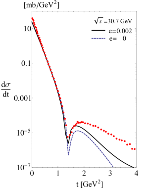
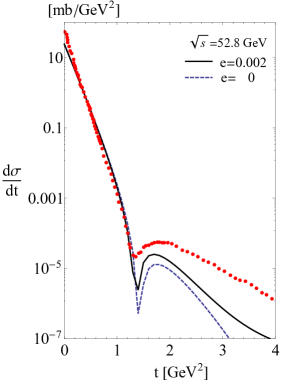
Figure 2: Elastic differential $pp$ cross section: solid (black) curve stringy pomeron with extrinsic curvature $\kappa=e=0.002$; dashed (blue) curve with $\kappa=e=0$; the data (red) is from Amaldi and Schubert (1980)..

V Conclusion

In holographic QCD the Pomeron exchange in dipole-dipole scattering with a large rapidity $\chi$ is described by the exchange of a non-critical string in hyperbolic $D=5$ dimensions. The extra (curved) direction is identified with the string scale dimension. In leading order, the Pomeron intercept is set by the Luscher-like term or $D_{\perp}/12$ Basar et al. (2012), and its slope is set by the string tension at the confinement scale. The curvature of the extra dimension causes the Pomeron intercept to shift from the Luscher term to order $1/\sqrt{\lambda}$ Stoffers and Zahed (2013a); Stoffers and Zahed (2012); Stoffers and Zahed (2013b).

Long color flux tubes in QCD are smooth. In leading order, the Nambu-Goto effective theory is corrected by a term that depends on the extrinsic curvature to allow for smooth string configurations  Polyakov (1986). The extrinsic curvature affects the zero point energy of large Wilson loops to one loop Hidaka and Pisarski (2009) and is amenable to lattice simulations. We have shown that a similar contribution affects the scattering amplitude of two dipoles. While there are higher order (loop) corrections to (IV.1), the retained contributions are leading in the Pomeron kinematics.

In leading order, the extrinsic curvature induces an overall momentum dependent contribution to the scattering amplitude. Detailed comparison with accurate but differential proton on proton measurements at large $\sqrt{s}$ but fixed $t=-{\bf q}_{\perp}^{2}$ show sensitivity of the diffractive peak to changes in the extrinsic curvature. $pp$ scattering may provide for an empirical estimate of the extrinsic curvatures of smooth QCD strings, besides the current measurement estimates for the slope (string tension) and intercept (Luscher contribution) of the Pomeron.

VI Acknowledgements

This work was supported by the U.S. Department of Energy under Contract No. DE-FG-88ER40388.

VII Appendix: Static and Stringy Dipole-Dipole Interaction

In this Appendix we detail the role of the extrinsic curvature on the correlator of two static but untwisted Wilson loops with $\theta=0$, i.e. the interaction between two static dipoles. Instead of (III.3) we now have the mode decomposition

$$x^{0}(\tau,\sigma) = \sum_{m=-\infty}^{\infty}\sum_{n=1}^{\infty}x_{m,n}^{0}\exp({i2\pi m\frac{\tau}{T}})\cos(\pi n\sigma)+X+\frac{P}{\sigma_{T}}\tau$$

$$x^{1}(\tau,\sigma) = \sum_{m=-\infty}^{\infty}\sum_{n=1}^{\infty}x_{m,n}^{1}\exp({i2\pi m\frac{\tau}{T}})\sin(\pi n\sigma)$$

$$x^{\perp}(\tau,\sigma) = (\sigma-\frac{1}{2})b^{\perp}+\sum_{m=-\infty}^{\infty}\sum_{n=1}^{\infty}x_{m,n}^{\perp}\exp({i2\pi m\frac{\tau}{T}})\sin(\pi n\sigma)$$ (7.0.1)

with $P$ the number of windings in the temporal direction. The exchanged closed string is assumed to be infinitely thin in this case in the absence of the boosting kinematics for the two scattering dipoles in the text. This approximation is justified in the final result (7.0.7-7.0.9) below. With this in mind, a repeat of the algebra in section III, yields the string partition function

$$\mathbb{K}(T,\kappa)=\mathbb{K}_{\rm F}(T)\,\,\exp\left(\frac{D_{\perp}}{4}Tb\sqrt{\kappa\sigma_{T}}\right)$$ (7.0.2)

with $\mathbb{K}_{\rm F}(T)$ the string propagator propagator without the extrinsic curvature in 3.1.1

$$\mathbb{K}_{\rm F}(T)=\frac{a^{2}}{\alpha^{\prime}}\exp\left(-\frac{\sigma_{T}}{2}Tb^{2}-\frac{TP^{2}}{2\sigma_{T}}\right)\left[\prod_{n=1}^{\infty}2\sinh\left(\frac{n\pi T}{2}\right)\right]^{-D_{\perp}}$$ (7.0.3)

In comparing to the result in Hidaka and Pisarski (2009), we note the occurrence of the same zero point energy (one loop)

$$E_{0}^{\rm non}=-\frac{D_{\perp}}{4}\sqrt{\sigma_{T}\kappa}$$ (7.0.4)

This is to be compared with our result (3.3.18) for the twisted dipoles, and shows the commonality between the untwisted and large Wilson loop and the twisted and far Wilson loops.

Now, we also notice that in our case

$$x^{0}(\tau+T,\sigma)=x^{0}(\tau,\sigma)+\frac{P}{\sigma_{T}}T$$ (7.0.5)

Thus $P=cW$ with $W=0,\pm 1,\pm 2,...$ with $W$ the winding number and $c$ a constant to be interpreted below. The propagators with different windings can be re-summed using the Poisson summation formula

$$\sum_{W=-\infty}^{\infty}\mathbb{K}(T,\kappa) = \sum_{W=-\infty}^{\infty}\frac{a^{2}}{\alpha^{\prime}}\exp\left(-\frac{\sigma_{T}}{2}Tb^{2}-W^{2}\frac{Tc^{2}}{2\sigma_{T}}+\frac{D_{\perp}}{4}Tb\sqrt{\kappa\sigma_{T}}\right)\left[\prod_{n=1}^{\infty}2\sinh\left(\frac{n\pi T}{2}\right)\right]^{-D_{\perp}}$$ (7.0.6)

$$= \sqrt{\frac{2\pi\sigma_{T}}{Tc^{2}}}\frac{a^{2}}{\alpha^{\prime}}\sum_{k=-\infty}^{\infty}\exp\left[-\frac{\sigma_{T}}{2}Tb^{2}\left(1-\frac{D_{\perp}\sqrt{\kappa}}{2b\sqrt{\sigma_{T}}}\right)-k^{2}\frac{2\pi^{2}\sigma_{T}}{Tc^{2}}\right]\eta^{-D_{\perp}}\left(i\frac{T}{2}\right)$$

where $\eta(\tau)$ is Dedekind eta function and $\eta(ix)=\eta(i/x)/\sqrt{x}~{}$Basar et al. (2012); Qian and Zahed (2012). Inserting(7.0.6) into (2.0.5) yields

$$\mathbb{WW} = \frac{g_{s}^{2}a^{2}}{4\alpha^{\prime}}\frac{\sqrt{\pi\sigma_{T}}}{|c|}\sum_{k=-\infty}^{\infty}\sum_{n=0}^{\infty}d(n)\int_{0}^{\infty}dT\,\,\left(\frac{T}{2}\right)^{\frac{D_{\perp}-3}{2}}$$ (7.0.7)

$$\ \ \ \ \ \ \ \ \ \ \ \ \ \ \ \ \ \ \ \ \ \ \ \ \ \ \ \ \ \ \ \ \ \ \ \ \ \times\exp\left[-\frac{T}{2}\sigma_{T}b^{2}\left(1-\frac{D_{\perp}\sqrt{\kappa}}{2b\sqrt{\sigma_{T}}}\right)-\frac{2}{T}k^{2}\frac{\pi^{2}\sigma_{T}}{c^{2}}\left(1+\frac{2n\pi c^{2}}{k^{2}\pi^{2}\sigma_{T}}-\frac{D_{\perp}c^{2}}{12k^{2}\pi\sigma_{T}}\right)\right]$$

$$= \frac{g_{s}^{2}a^{2}\sqrt{\sigma_{T}}}{\alpha^{\prime}}\left(\frac{\pi}{|c|}\right)^{\frac{D_{\perp}}{2}}\sum_{k=-\infty}^{\infty}\sum_{n=0}^{\infty}d(n)\left(\frac{1+\frac{2n\pi c^{2}}{k^{2}\pi^{2}\sigma_{T}}-\frac{D_{\perp}c^{2}}{12k^{2}\pi\sigma_{T}}}{1-\frac{D_{\perp}\sqrt{\kappa}}{2b\sqrt{\sigma_{T}}}}\right)^{\frac{D_{\perp}-1}{4}}\left(\frac{k}{b}\right)^{\frac{D_{\perp}-1}{2}}$$

$$\ \ \ \ \ \ \ \ \ \ \ \ \ \ \ \ \ \ \ \ \ \ \ \ \ \ \ \ \ \ \ \ \ \ \ \ \ \times\mathbb{K}_{\frac{D_{\perp}-1}{2}}\left(\frac{2bk\pi\sigma_{T}}{|c|}\sqrt{\left(1-\frac{D_{\perp}\sqrt{\kappa}}{2b\sqrt{\sigma_{T}}}\right)\left(1+\frac{2n\pi c^{2}}{k^{2}\pi^{2}\sigma_{T}}-\frac{D_{\perp}c^{2}}{12k^{2}\pi\sigma_{T}}\right)}\right)$$

which is the correlator between two static dipoles at large distances $b\gg D_{\perp}\sqrt{\kappa/4\sigma_{T}}$. The summation over $k$ should be limited to $k=[N_{c}/2]=1$ for dipoles in the fundamental representation of SU(N_c) Qian and Zahed (2012). $d(n)$ is the canonical string density of states with $d(0)=1$. The static dipole-dipole potential following from the smooth string exchange, amounts to a tower of scalar exchanges with masses ($k=1$)

$$m_{n}(b,c)=\frac{2\pi\sigma_{T}}{|c|}\sqrt{\left(1-\frac{D_{\perp}\sqrt{\kappa}}{2b\sqrt{\sigma_{T}}}\right)\left(1+\frac{2n\pi c^{2}}{\pi^{2}\sigma_{T}}-\frac{D_{\perp}c^{2}}{12\pi\sigma_{T}}\right)}$$ (7.0.8)

at large distances $b\gg D_{\perp}\sqrt{\kappa/4\sigma_{T}}$. Without the extrinsic curvature and setting $|c|\equiv 2\pi/\beta$, $m_{n}$ is the mass spectrum for closed strings of (arbitrary) size $\beta>\beta_{H}$,

$$m_{n}(\infty,2\pi/\beta)=\sigma_{T}\beta\sqrt{1-\frac{\beta_{H}^{2}}{\beta^{2}}+\frac{8\pi n}{\sigma_{T}\beta^{2}}}$$ (7.0.9)

with the Hagedorn temperature $\beta_{H}=\sqrt{\pi D_{\perp}/3\sigma_{T}}$. Here $1/\beta=|c|/2\pi$ plays the role of an effective temperature associated with the exchange of a closed (periodic) string.

Phys.Lett.,B373,210 Phys.Lett.,B429,107

References

• Gribov et al. (1983) L. Gribov, E. Levin, and M. Ryskin, Phys.Rept. 100, 1 (1983).
• Kuraev et al. (1976) E. A. Kuraev, L. N. Lipatov, and V. S. Fadin, Sov.Phys.JETP 44, 443 (1976).
• Lipatov (1976) L. Lipatov, Sov.J.Nucl.Phys. 23, 338 (1976).
• Sterman (1999) G. F. Sterman (1999), eprint hep-ph/9905548.
• Fadin et al. (1975) V. S. Fadin, E. Kuraev, and L. Lipatov, Phys.Lett. B60, 50 (1975).
• Balitsky and Lipatov (1978) I. Balitsky and L. Lipatov, Sov.J.Nucl.Phys. 28, 822 (1978).
• Veneziano (1968) G. Veneziano, Nuovo Cim. A57, 190 (1968).
• Greensite (1985) J. Greensite, Nucl.Phys. B249, 263 (1985).
• Maldacena (1998) J. M. Maldacena, Phys.Rev.Lett. 80, 4859 (1998), eprint hep-th/9803002.
• Rho et al. (1999) M. Rho, S.-J. Sin, and I. Zahed, Phys.Lett. B466, 199 (1999), eprint hep-th/9907126.
• Janik and Peschanski (2000) R. Janik and R. B. Peschanski, Nucl.Phys. B586, 163 (2000), eprint hep-th/0003059.
• Janik (2001) R. A. Janik, Phys.Lett. B500, 118 (2001), eprint hep-th/0010069.
• Polchinski and Strassler (2002) J. Polchinski and M. J. Strassler, Phys.Rev.Lett. 88, 031601 (2002), eprint hep-th/0109174.
• Polchinski and Strassler (2003) J. Polchinski and M. J. Strassler, JHEP 0305, 012 (2003), eprint hep-th/0209211.
• Brower et al. (2007) R. C. Brower, J. Polchinski, M. J. Strassler, and C.-I. Tan, JHEP 0712, 005 (2007), eprint hep-th/0603115.
• Brower et al. (2009) R. C. Brower, M. J. Strassler, and C.-I. Tan, JHEP 0903, 092 (2009), eprint 0710.4378.
• Brower et al. (2010) R. C. Brower, M. Djuric, I. Sarcevic, and C.-I. Tan, JHEP 1011, 051 (2010), eprint 1007.2259.
• Brower et al. (2011) R. C. Brower, M. Djuric, I. Sarcevic, and C.-I. Tan (2011), eprint 1106.5681.
• Hatta et al. (2008a) Y. Hatta, E. Iancu, and A. Mueller, JHEP 0801, 063 (2008a), eprint 0710.5297.
• Hatta et al. (2008b) Y. Hatta, E. Iancu, and A. Mueller, JHEP 0801, 026 (2008b), eprint 0710.2148.
• Albacete et al. (2008) J. L. Albacete, Y. V. Kovchegov, and A. Taliotis, JHEP 0807, 074 (2008), eprint 0806.1484.
• Albacete et al. (2009) J. L. Albacete, Y. V. Kovchegov, and A. Taliotis, AIP Conf.Proc. 1105, 356 (2009), eprint 0811.0818.
• Basar et al. (2012) G. Basar, D. E. Kharzeev, H.-U. Yee, and I. Zahed, Phys.Rev. D85, 105005 (2012), eprint 1202.0831.
• Stoffers and Zahed (2013a) A. Stoffers and I. Zahed, Phys.Rev. D87, 075023 (2013a), eprint 1205.3223.
• Stoffers and Zahed (2012) A. Stoffers and I. Zahed (2012), eprint 1210.3724.
• Stoffers and Zahed (2013b) A. Stoffers and I. Zahed, Acta Phys.Polon.Supp. 6, 7 (2013b).
• Qian and Zahed (2012) Y. Qian and I. Zahed (2012), eprint 1211.6421.
• Shuryak and Zahed (2014) E. Shuryak and I. Zahed, Phys.Rev. D89, 094001 (2014), eprint 1311.0836.
• Brodsky et al. (2013) S. J. Brodsky, G. F. de Téramond, and H. G. Dosch, Nuovo Cim. C036, 265 (2013), eprint 1302.5399.
• Polyakov (1986) A. M. Polyakov, Nucl.Phys. B268, 406 (1986).
• Kuti (2006) J. Kuti, PoS LAT2005, 001 (2006), eprint hep-lat/0511023.
• Hidaka and Pisarski (2009) Y. Hidaka and R. D. Pisarski, Phys.Rev. D80, 074504 (2009), eprint 0907.4609.
• Amaldi and Schubert (1980) U. Amaldi and K. R. Schubert, Nucl.Phys. B166, 301 (1980).
• Amaldi et al. (1971) U. Amaldi, R. Biancastelli, C. Bosio, G. Matthiae, J. Allaby, et al., Phys.Lett. B36, 504 (1971).