Loop quantization of a 3D Abelian BF model
with $\sigma$-model matter

Abstract

The main goal of this work is to explore the symmetries and develop the dynamics associated to a 3D Abelian BF model coupled to scalar fields submitted to a sigma model like constraint, at the classical and quantum levels. We adapt to the present model the techniques of Loop Quantum Gravity, construct its physical Hilbert space and its observables.

1 Introduction

The now quasi-hundred years old General Relativity as a theory of gravitation, despite of its tremendous successes in accounting for predicting phenomena, still lacks of a quantum version. Previous perturbative attempts have shown the non-renormalizability of the theory [1], whereas the pioneering non-perturbative approach of Wheeler and DeWitt [2] had its successes concentrated in reduced “minisuperspace” models dedicated to Cosmology. However, very important progresses have been made in the last decades, especially in the framework of Loop Quantum Gravity (LQG) [3], based on the canonical Hamiltonian approach of Dirac and Bergman [4] applied to the Ashtekar-Barbero [5, 6] parametrization of the theory. General Relativity, as a background independent theory – in the sense that no background geometry is given a priori, geometry being dynamical – is a fully constrained theory, its Hamiltonian being merely a sum of constraints generating the gauge invariances of the theory. The LQG program entails the difficult task of implementing the constraints of the theory as quantum operators in some predefined kinematic Hilbert space, and to solve them, thus leaving as a subspace the physical Hilbert space in which act the self-adjoint operators representing the observables of the theory. Some of the constraints have been resolved, but a last one, the so-called scalar constraint. The latter has resisted up to now a complete solution, the most popular approach being that of “spin foams” [7, 8].

By contrast, the lower-dimensional gravitation theories are much more easy to handle, since they can be described as topological gauge theories, when not coupled to matter [9, 10, 11, 12, 13]. Coupling them to matter however lets them loose their topological character, excepted in some special cases, where a complete and rather simple loop quantization can be achieved [14, 15].

The purpose of this paper is to present the loop quantization of a topological theory of the BF type [16] with the Abelian group U(1) as a gauge group. The BF fields are coupled to a complex scalar “matter” field subject to a $\sigma$-model type of constraint. It turns out that the topological nature of the theory persists in the sense that no local degrees of freedom are present. The physical Hilbert space is constructed with a non-trivial result if the topology of space is non-trivial. Spaces with point-like singularities are considered, in which cases global observables are explicitly constructed. A non-Abelian version is presently under study [15].

The model and its gauge invariances is presented in Section 2, its classical analysis is done in Section 3 together with the separation of the first and second class constraints and the definition of the Dirac brackets, and the quantization is presented in Section 4. Brief conclusions are given at last.

2 Formulation of the model

2.1 The gauge invariances and the action

The field content of the model is a U(1) connection form $A=A_{\mu}(x)dx^{\mu}$, a “B” form $B=B_{\mu}(x)dx^{\mu}$, a complex scalar field ${\phi}(x)$ and a 3-form field $e=\frac{1}{3!}e_{\mu\nu\rho}dx^{\mu}dx^{\nu}dx^{\rho}$, transforming as

$$A_{\mu}^{\prime}=A_{\mu}^{\prime}+g^{-1}\partial_{\mu}g=A_{\mu}+\partial_{\mu}\theta\,,\quad B^{\prime}=B\,,\quad{\phi}^{\prime}=g{\phi}\,,\quad{\bar{{\phi}}}^{\prime}=g^{-1}{\bar{{\phi}}}\,,\quad e^{\prime}=e\,,$$ (2.1)

under U(1) gauge transformations $g(x)=\exp\theta(x)$

One introduces also the topological type gauge transformations

$$A^{\prime}=A\,,\quad B^{\prime}=B+d\psi\,,\quad{\phi}^{\prime}={\phi}\,,\quad e^{\prime}=e-d\psi F\,,$$ (2.2)

where $F=dA$ and the scalar $\psi(x)$ is the transformation parameter. These transformations coincide with the usual topological type transformations of the $BF$ model, in the absence of the fields ${\phi}$ and $e$.

The most general action invariant under the sole gauge transformations (2.1) can be written as

$$S_{\rm general}={\displaystyle{\int}\!\!\!}_{{\cal M}^{3}}\left(K(\bar{\phi}{\phi})BF+\lambda(\bar{\phi}{\phi})BD\bar{\phi}D{\phi}+e[\mu(\bar{\phi}{\phi})-R]\right)\,,$$

where $K,\,\lambda$ and $\mu$ are arbitrary functions of $\bar{\phi}{\phi}$, and $D$ denotes the covariant derivative(covariant with respect to the gauge transformation (2.1)):

$$D{\phi}=(d-A){\phi}\,,\quad D\bar{\phi}=(d+A)\bar{\phi}\,.$$

The integration is performed over some 3D differential manifold ${\cal M}^{3}$. The action is obviously invariant under the diffeomorphisms of ${\cal M}^{3}$.

The parameter $R$ can be taken equal to 1 through a renormalization of the field $e$, and one easily shows that one can reduce the function $\mu(\bar{\phi}{\phi})$ to the form $\mu=\bar{\phi}{\phi}$ through a suitable field redefinition $\phi\to\phi^{\prime}(\phi,\bar{\phi})$, $\bar{\phi}\to\bar{\phi}^{\prime}(\phi,\bar{\phi})$, compatible with the gauge transformation (2.1). Imposing now the topological gauge invariance $(\ref{transf-psi})$ fixes the function $\lambda$ to the constant value 1. The action then reads

$${\displaystyle{\int}\!\!\!}_{{\cal M}^{3}}\left(K(\bar{\phi}{\phi})BF+BD\bar{\phi}D{\phi}+e(\bar{\phi}{\phi}-1)\right)\,.$$

The resulting field equation $\bar{\phi}{\phi}=1$ implies that the function $K$ can be replaced by a constant, which in turn can be reabsorbed through a renormalization of the field $B$. The final action is then

$$S={\displaystyle{\int}\!\!\!}_{{\cal M}^{3}}\left(BF+BD\bar{\phi}D{\phi}+e(\bar{\phi}{\phi}-1)\right)\,.$$ (2.3)

One recognizes in (2.3) a $BF$ action coupled with scalar fields and a Lagrange multiplier field $e$ assuring the $\sigma$-model type constraint $\bar{\phi}{\phi}=1$.

It turns out that the action (2.3) has a third gauge invariance: It is invariant under the following local transformations, of parameter $\eta(x)$:

$$A^{\prime}=A+d\eta\,,\quad B^{\prime}=B\,,\quad,{\phi}^{\prime}={\phi}\,,\quad e^{\prime}=e+d\eta\,dB\,.$$ (2.4)

In order to check the invariances of the action (up to boundary terms), as well as for all the manipulations involving partial integrations, it is useful to remember that the covariant derivative $D$, defined by $DX=dX-qAX$ where $q$ is the U(1) charge of the field X, obeys the Leibniz rule. The respective U(1) charges of the basic fields $A,B,{\phi},\bar{\phi}$ and $e$ are $0,0,1,-1$ and 0. Let us also note the useful identity

$$D\bar{\phi}D{\phi}=d\bar{\phi}d{\phi}+A\,d(\bar{\phi}{\phi})\,.$$

The field equations read

$$\begin{array}[]{ll}{\displaystyle{\frac{\delta S}{\delta B}}}=F+D\bar{\phi}D{\phi}\stackrel{{\scriptstyle*}}{{=}}0\,,&{\displaystyle{\frac{\delta S}{\delta A}}}={}dB-Bd(\bar{\phi}{\phi})\stackrel{{\scriptstyle*}}{{=}}0\,,\\[8.53581pt] {\displaystyle{\frac{\delta S}{\delta\bar{\phi}}}}=BF{\phi}-dBD{\phi}+e{\phi}\stackrel{{\scriptstyle*}}{{=}}0\,,&{\displaystyle{\frac{\delta S}{\delta{\phi}}}}=BF\bar{\phi}-dBD\bar{\phi}+e\bar{\phi}\stackrel{{\scriptstyle*}}{{=}}0\,,\\[8.53581pt] {\displaystyle{\frac{\delta S}{\delta e}}}=\bar{\phi}{\phi}-1\stackrel{{\scriptstyle*}}{{=}}0\,,\end{array}$$

where the symbol $\stackrel{{\scriptstyle*}}{{=}}$ means “on shell” equality, i.e., “equations of motion being fulfilled”. The last equation is equivalent to

$${\phi}(x)\stackrel{{\scriptstyle*}}{{=}}e^{i{\varphi}(x)}\,,\quad{\bar{{\phi}}}(x)\stackrel{{\scriptstyle*}}{{=}}e^{-i{\varphi}(x)}\,,\quad{\varphi}\mbox{ a real phase}\,.$$ (2.5)

This system of equations is equivalent to the simpler one:

$$F\stackrel{{\scriptstyle*}}{{=}}0\,,\quad dB\stackrel{{\scriptstyle*}}{{=}}0\,,\quad e\stackrel{{\scriptstyle*}}{{=}}0\,,\quad\bar{\phi}{\phi}-1\stackrel{{\scriptstyle*}}{{=}}0\,.$$

2.2 Diffeomorphism invariance

In the present theory, like in the topological theories of the Chern-Simons or $BF$ type, the invariance under the diffeomorphisms is a consequence of the invariance under the gauge transformations (2.1), (2.2) and (2.4), up to field equations. Indeed, the diffeomorphisms being generated by the Lie derivative ${\cal L}_{\xi}=i_{\xi}d+di_{\xi}$ along an infinitesimal vector field $\xi$ when acting on forms, one checks that

$$\begin{array}[]{ll}{\cal L}_{\xi}A\stackrel{{\scriptstyle*}}{{=}}d(i_{\xi}A)\,,&{\cal L}_{\xi}B=d(i_{\xi}B)\,,\\[8.53581pt] {\cal L}_{\xi}{\phi}\stackrel{{\scriptstyle*}}{{=}}i(i_{\xi}d{\varphi}){\phi}\,,&\quad{\cal L}_{\xi}{\bar{{\phi}}}\stackrel{{\scriptstyle*}}{{=}}-i(i_{\xi}d{\varphi}){\bar{{\phi}}}\,,\quad{\cal L}_{\xi}e\stackrel{{\scriptstyle*}}{{=}}0\,,\end{array}$$

where ${\varphi}$ is the phase of the field ${\phi}$ defined in (2.5). One sees that these infinitesimal diffeomorphisms are given, on-shell, by a combination of the three gauge invariances, with the respective field dependent infinitesimal parameters given by

$$\theta=i(i_{\xi}d{\varphi})\,,\quad\psi=i_{\xi}B\,,\quad\eta=i_{\xi}(A-id{\varphi})\,.$$

3 Hamiltonian analysis and constraints

We apply here the canonical formalism of Dirac [4] for systems with constraints. Supposing that the space-time manifold admits a “time” $\times$ “space” foliation ${\cal M}_{3}=\mathbb{R}\times\Sigma$, where the space slice $\Sigma$ is some two-dimensional manifold, we first rewrite the action as the time integral

$$S=\int dt\,L(A,\dot{A},B,\dot{B},{\phi},\dot{\phi},\bar{\phi},\dot{\bar{\phi}},e,\dot{e})$$

of a Lagrangian function

$$\begin{array}[]{l}L(A,\dot{A},B,\dot{B},{\phi},\dot{\phi},\bar{\phi},\dot{\bar{\phi}},e,\dot{e})=\\[8.53581pt] \ {\displaystyle{\int}\!\!\!}_{\Sigma}d^{2}x\left({}{\tilde{B}}^{a}\partial_{t}A_{a}-{\tilde{B}}^{a}D_{a}\bar{\phi}\,\partial_{t}{\phi}+{\tilde{B}}^{a}D_{a}{\phi}\,\partial_{t}\bar{\phi}+A_{t}{\cal C}_{1}+B_{t}{\cal C}_{2}+{\tilde{e}}{\cal C}_{5}\right)\,,\end{array}$$ (3.1)

where

$$\begin{array}[]{l}{\cal C}_{1}={}\partial_{a}{\tilde{B}}^{a}+{\tilde{B}}^{a}\partial_{a}(\bar{\phi}{\phi})\\[8.53581pt] {\cal C}_{2}={}{\tilde{F}}+\varepsilon^{ab}D_{a}\bar{\phi}D_{b}{\phi}\\[8.53581pt] {\cal C}_{5}=\bar{\phi}{\phi}-1\,,\\[8.53581pt] {\tilde{F}}=\frac{1}{2}\varepsilon^{ab}F_{ab}\,,\quad{\tilde{B}}^{a}=\varepsilon^{ab}B_{b}\,,\quad{\tilde{e}}=\frac{1}{3!}\varepsilon^{\mu\nu\rho}e_{\mu\nu\rho}\,.\end{array}$$ (3.2)

Following the canonical procedure, we identify the conjugate momenta of each field $X$, $\Pi_{X}=\delta{L}/\delta{\dot{X}}$:

$$\begin{array}[]{l}\Pi_{A_{t}}=0\,,\quad\Pi_{B_{t}}=0\,,\quad\Pi_{{\tilde{e}}}=0\,,\Pi_{{\phi}}=-{\tilde{B}}^{a}D_{a}\bar{\phi}\,,\quad\Pi_{\bar{\phi}}={\tilde{B}}^{a}D_{a}{\phi}\,,\\[8.53581pt] \Pi_{A_{a}}={\tilde{B}}^{a}\,,\quad\Pi_{B_{a}}=0\,,\end{array}$$ (3.3)

satisfying together with the $X$’s the equal time Poisson bracket relations

$$\{X^{\alpha}({\boldsymbol{x}}),\Pi_{X^{\beta}}({\boldsymbol{y}})\}=\delta^{\alpha}_{\beta}\delta^{2}({\boldsymbol{x}},{\boldsymbol{y}})\,,\quad\{X^{\alpha}({\boldsymbol{x}}),X^{\beta}({\boldsymbol{y}})\}=\{\Pi_{X^{\alpha}}({\boldsymbol{x}}),\Pi_{X^{\beta}}({\boldsymbol{y}})\}=0\,,$$

where the indices $\alpha,\beta$ run over all components of all fields. The Legendre transform $H_{\rm c}=-L+\sum_{\alpha}\int d^{2}x\,\Pi_{X^{\alpha}}{\dot{X}}^{\alpha}$ yields the canonical Hamiltonian

$$H_{\rm c}=-\int d^{2}x\left(A_{t}{\cal C}_{1}+B_{t}{\cal C}_{2}+{\tilde{e}}{\cal C}_{5}\right)\,,$$

with the ${\cal C}$’s given in (3.2).

Noting that the velocities don’t appear in any of the equations (3.3) for the momenta, we conclude that all of these equations are (primary) constraints [4]. The equality sign must be replaced by the “weak equality” sign $\approx$, meaning that the constraints are solved at the end, after all calculations involving Poisson brackets are done. We remark that the last two constraints in (3.3) are second class, their brackets being non-zero: $\{\Pi_{A_{a}}({\boldsymbol{x}})-\varepsilon^{ab}B_{b}({\boldsymbol{x}}),\,\Pi_{B_{c}}({\boldsymbol{y}})\}$ $=$ $\varepsilon^{ab}\delta^{2}({\boldsymbol{x}},{\boldsymbol{y}})$. These constraints can be solved as strong equalities

$$\Pi_{A_{a}}=\varepsilon^{ab}B_{b}={\tilde{B}}^{a}\,,\quad\Pi_{B_{a}}=0\,,$$ (3.4)

provided the Poisson Brackets are replaced by the corresponding Dirac brackets, which read

$$\{A_{a}({\boldsymbol{x}}),\,{\tilde{B}}^{b}({\boldsymbol{y}})\}=\delta^{b}_{a}\delta^{2}({\boldsymbol{x}},{\boldsymbol{y}})\,,$$

the other brackets being left unchanged. We use the same notation $\{\cdot,\cdot\}$ for these Dirac brackets.

We are left with the five constraints

$$\Pi_{A_{t}}\approx 0\,,\quad\Pi_{B_{t}}\approx 0\,,\quad\Pi_{{\tilde{e}}}\approx 0\,,$$ (3.5)

and

$${\cal C}_{3}({\boldsymbol{x}})=\Pi_{{\phi}}+{\tilde{B}}^{a}D_{a}\bar{\phi}\approx 0\,,\quad{\cal C}_{4}({\boldsymbol{x}})=\Pi_{\bar{\phi}}-{\tilde{B}}^{a}D_{a}{\phi}\approx 0\,.$$ (3.6)

The stability of the three constraints (3.5) under the Hamiltonian evolution requires the three secondary constraints

$${\cal C}_{1}({\boldsymbol{x}})\approx 0\,,\quad{\cal C}_{2}({\boldsymbol{x}})\approx 0\,,\quad{\cal C}_{5}({\boldsymbol{x}})\approx 0\,,\quad\,,$$ (3.7)

with ${\cal C}_{1}$, ${\cal C}_{2}$ and ${\cal C}_{5}$ as given in (3.2). It will turn out convenient to replace ${\cal C}_{1}$ by the equivalent constraint:

$${\cal C}^{\prime}_{1}({\boldsymbol{x}})\approx 0\,,\quad\mbox{with}\quad{\cal C}^{\prime}_{1}({\boldsymbol{x}})={\cal C}_{1}-{\phi}{\cal C}_{3}+{\bar{{\phi}}}{\cal C}_{4}=\partial_{a}{\tilde{B}}^{a}-{\phi}\Pi_{\phi}+{\bar{{\phi}}}\Pi_{\bar{{\phi}}}\,.$$ (3.8)

The constraints (3.5) can be put strongly to zero, the corresponding fields $A_{t}$, $B_{t}$ and ${\tilde{e}}$ playing now the roles of Lagrange multipliers $\lambda_{1}$, $\lambda_{2}$ and $\lambda_{5}$. Introducing also Lagrange multipliers fields for the primary constraints (3.6), we define the total Hamiltonian as

$$H_{\rm T}=\sum_{m=1}^{5}{\cal C}_{m}[\lambda_{m}]\,,$$ (3.9)

where we have defined the functionals

$${\cal C}_{m}[\lambda_{m}]=\int d^{2}x\,\lambda_{m}({\boldsymbol{x}}){\cal C}_{m}({\boldsymbol{x}})\,,$$ (3.10)

considering the Lagrangian multiplier fields $\lambda_{m}$ as smooth test functions.

Since this Hamiltonian is entirely made of constraints – a characteristics of theories with general covariance – the stability of our five constraints ${\cal C}_{\alpha}$, $\alpha=1,\cdots,5$ amounts to examine the matrix $M_{mn}({\boldsymbol{x}},{\boldsymbol{y}})$ $\approx$ $\{{\cal C}_{m}(x),{\cal C}_{n}(y)\}$ of their Poisson brackets – written up to constraints, hence the $\approx$ sign. Indeed, their stability condition reads (summation convention is assumed)

$$\dot{\cal C}_{m}=\{{\cal C}_{m},H_{\rm T}\}=M_{mn}\lambda^{n}=0\,.$$ (3.11)

This provides a system of equations for the $\lambda$’, which can be solved for some of the $\lambda$’s in terms of the remaining ones. The matrix $M$ reads

$$M=\left(\begin{array}[]{ccccc}0&0&0&0&0\\ 0&0&0&{\phi}{\cal C}_{2}&0\\ 0&0&0&-({\phi}{\cal C}_{1}^{\prime}+{\cal C}_{3})&0\\ 0&-{\phi}{\cal C}_{2}&({\phi}{\cal C}_{1}^{\prime}+{\cal C}_{3})&0&-{\phi}\\ 0&0&0&{\phi}&0\end{array}\right)\delta^{2}({\boldsymbol{x}}-{\boldsymbol{y}})\,,$$

where we have substituted the constraint ${\cal C}_{3}$ with the equivalent one

$${\cal C}_{3}^{\prime}={\phi}\,{\cal C}_{3}-\bar{\phi}\,{\cal C}_{4}\,.$$

One sees that the first three constraints, ${\cal C}_{1}$, ${\cal C}_{2}$ and ${\cal C}^{\prime}_{3}$ are first class, i.e., their Poisson brackets with any other constraint are constraints: they generate three gauge invariances of the theory. The two last ones, namely ${\cal C}_{4}$ and ${\cal C}_{5}$ however are second class. Indeed, denoting them by $\chi_{p}$ ($p=1,2$), their Poisson brackets form the matrix $C_{pq}$ of non-vanishing determinant on the constraint surface:

$$C=\left(\begin{array}[]{cc}0&-{\phi}\\ {\phi}&0\end{array}\right)\,.$$

These second class constraints may be written as strong equalities, provided the Poisson brackets are substituted by the Dirac brackets [4]

$$\{X,Y\}_{\rm D}=\{X,Y\}-\sum_{p,q}\{X,\chi_{p}\}(C^{-1})^{pq}\{\chi_{q},Y\}\,.$$ (3.12)

The second class constraints $\chi_{p}$ can be solved for ${\bar{{\phi}}}$ and $\Pi_{{\bar{{\phi}}}}$ in terms of the now independent fields $A_{a}$, ${\tilde{B}}^{a}$, ${\phi}$ and $\Pi_{\phi}$,

$${\bar{{\phi}}}=1/{\phi}\,,\quad\Pi_{{\bar{{\phi}}}}={\tilde{B}}^{a}D_{a}{\phi}\,.$$

The independent fields obey the Dirac bracket relations

$$\begin{array}[]{ll}\{A_{a}({\boldsymbol{x}}),{\tilde{B}}^{b}({\boldsymbol{y}})\}_{\rm D}=\delta^{b}_{a}\,\delta^{2}({\boldsymbol{x}}-{\boldsymbol{y}})\,,&\{{\phi}({\boldsymbol{x}}),\Pi_{\phi}({\boldsymbol{y}})\}_{\rm D}=\delta^{2}({\boldsymbol{x}}-{\boldsymbol{y}})\,,\\[8.53581pt] \{A_{a}({\boldsymbol{x}}),\Pi_{\phi}({\boldsymbol{y}})\}_{\rm D}=D_{a}\left({\displaystyle{\frac{1}{{\phi}}}}\right)\,\delta^{2}({\boldsymbol{x}}-{\boldsymbol{y}})\,,&\{{\tilde{B}}^{a}({\boldsymbol{x}}),\Pi_{\phi}({\boldsymbol{y}})\}_{\rm D}=-{\tilde{B}}^{a}{\displaystyle{\frac{1}{{\phi}}}}\delta^{2}({\boldsymbol{x}}-{\boldsymbol{y}})\,,\\[8.53581pt] \mbox{(other brackets vanishing)}\,.\end{array}$$

This system can be diagonalized through the redefinition

$$\Pi=\Pi_{\phi}-{\tilde{B}}^{a}D_{a}\left({\displaystyle{\frac{1}{{\phi}}}}\right)\,,$$ (3.13)

with the result:

$$\begin{array}[]{l}\{A_{a}({\boldsymbol{x}}),{\tilde{B}}^{b}({\boldsymbol{y}})\}_{\rm D}=\delta^{b}_{a}\,\delta^{2}({\boldsymbol{x}}-{\boldsymbol{y}})\,,\quad\{{\phi}({\boldsymbol{x}}),\Pi({\boldsymbol{y}})\}_{\rm D}=\delta^{2}({\boldsymbol{x}}-{\boldsymbol{y}})\,,\\[8.53581pt] \mbox{(other brackets vanishing)}\,.\end{array}$$ (3.14)

Finally, the remaining three constraints read, taking (3.13) into account:

$${\cal C}_{1}=\partial_{a}{\tilde{B}}^{a}\,,\quad{\cal C}_{2}={\tilde{F}},\quad{\cal C}_{3}={\Phi}\Pi\,.$$ (3.15)

They are first class (their Dirac brackets are indeed zero), and generate the three gauge invariances defined by $\delta_{i}X$ $=$ $\{X,{\cal C}_{i}[\epsilon_{i}]\}$ ($i=1,2,3$) using the functional notation (3.10):

$$\begin{array}[]{lll}\delta_{1}A_{a}=-\partial_{a}\epsilon_{1}\,,&\delta_{2}A_{a}=0\,,&\delta_{3}A_{a}=0\,,\\[8.53581pt] \delta_{1}{\tilde{B}}^{a}=0\,,&\delta_{2}{\tilde{B}}^{a}=-\epsilon^{ab}\partial_{b}\epsilon_{2}\,,&\delta_{3}{\tilde{B}}^{a}=0\,,\\[8.53581pt] \delta_{1}{\phi}=0\,,&\delta_{2}{\phi}=0\,,&\delta_{3}{\phi}=\epsilon_{3}{\phi}\,,\\[8.53581pt] \delta_{1}\Pi=0\,,&\delta_{2}\Pi=0\,,&\delta_{3}\Pi=-\epsilon_{3}\Pi\,.\end{array}$$ (3.16)

We see that the U(1) gauge invariance is split in two invariances generated by ${\cal C}_{1}$ and ${\cal C}_{3}$, corresponding to the invariances (2.1) and (2.4) of the Lagrangian formalism. The invariance generated by ${\cal C}_{2}$ corresponds to the topological type invariance (2.2).

4 Quantization

4.1 Kinematical Hilbert space

The constraints ${\cal C}_{1}$ and ${\cal C}_{3}$ will be solved at the quantum level in this Section, whereas the last one, ${\cal C}_{2}$, is left for the next Section. Following the lines of Loop Quantum Gravity [3], we shall construct a kinematical Hilbert space ${\cal H}_{\rm kin}$ whose vectors $\left|{\Psi}\right\rangle$ are subjected to the constraints ${\cal C}_{1}$ and ${\cal C}_{3}$ in the form $\hat{\cal C}_{1}\left|{\Psi}\right\rangle=0$ and $\hat{\cal C}_{3}\left|{\Psi}\right\rangle=0$, where $\hat{\cal C}_{i}$ are operators representing the classical ${\cal C}_{i}$. Choosing the fields $A_{a}$ and ${\phi}$ as configuration space coordinates, our task will be to define wave functionals $\Psi[A,{\phi}]$ and the scalar product $\langle{\Psi|\Psi^{\prime}}\rangle$. The fields are now promoted to operators $\hat{A}_{a}$, $\hat{\phi}$, $\hat{B}^{a}$ and $\hat{\Pi}$ obeying the canonical commutation relations corresponding to the classical Dirac brackets(3.14):

$$\begin{array}[]{l}[\hat{A}_{a}({\boldsymbol{x}}),\hat{B}^{b}({\boldsymbol{y}})]=i\hbar\delta^{b}_{a}\,\delta^{2}({\boldsymbol{x}}-{\boldsymbol{y}})\,,\quad[\hat{\phi}({\boldsymbol{x}}),\hat{\Pi}({\boldsymbol{y}})]=i\hbar\delta^{2}({\boldsymbol{x}}-{\boldsymbol{y}})\,,\\[8.53581pt] \mbox{(other brackets vanishing)}\,.\end{array}$$ (4.1)

$\hat{A}$ and $\hat{\phi}$ act multiplicatively, $\hat{B}$ and $\hat{\Pi}$ as functional derivatives:

$$\hat{B}^{a}({\boldsymbol{x}})\Psi[A,{\phi}]=-i\hbar{\displaystyle{\frac{\delta\Psi[A,{\phi}]}{\delta A_{a}({\boldsymbol{x}})}}}\,,\quad\hat{\Pi}({\boldsymbol{x}})\Psi[A,{\phi}]=-i\hbar{\displaystyle{\frac{\delta\Psi[A,{\phi}]}{\delta{\phi}({\boldsymbol{x}})}}}$$

Everything up to now is purely formal since we have still no proper Hilbert space. But we can already solve the constraint $\hat{\cal C}_{3}({\boldsymbol{x}})\Psi[{\phi},A]$ = $-i\hbar\hat{\phi}\,\delta\Psi[{\phi},A]/\delta{\phi}({\boldsymbol{x}})$ $=0$: the wave functional only depends on $A$, $\Psi$ = $\Psi[A]$.

In order to construct a scalar product defined by an appropriate integration measure in configuration space, we first restrict the space of wave functionals to the set of functions of finite numbers of holonomies of the connection $A$ – the “cylindrical functions”. If $\gamma$ is an orientated curve in $\Sigma$ (a “link”), the holonomy of $A$ on $\gamma$ is defined as the exponentiated line integral

$$h_{\gamma}[A]=\exp{\int_{\gamma}A}\,.$$ (4.2)

Given a “graph”, i.e., a finite set $\Gamma=\{\gamma_{1},\cdots,.\gamma_{N}\}$ of links, a “cylindrical function” $\Psi_{\Gamma,\psi}[A]$ is function $\psi$ of the holonomies of $\Gamma$:

$$\Psi_{\Gamma,\psi}[A]=\psi(h_{\gamma_{1}}[A],\cdots,h_{\gamma_{N}}[A])\,.$$

The cylindrical functions associated to all graphs on $\Sigma$ form the vectorial space Cyl, in which we can define a sesquilinear scalar product using the Haar measure $d\mu(g)$ of the gauge group. For U(1), the (normalized) measure is given by $\frac{1}{2\pi}\int d\theta f(g(\theta))$ for $g$ parametrized as $g(\theta)=\exp(i\theta)$. First, for two cylindrical functions defined on the same graph:

$$\langle{\Gamma,\psi|\Gamma,\psi^{\prime}}\rangle=\int_{G^{\otimes N}}\int d\mu(g_{1})\,\cdots d\mu(g_{N})(\psi(g_{1},\cdots,g_{N}))^{*}\psi^{\prime}(g_{1},\cdots,g_{N})\,.$$

Next, for two cylindrical functions corresponding to two different graph $\Gamma$ and $\Gamma^{\prime}$, one defines

$$\langle{\Gamma,\psi|\Gamma^{\prime},\psi^{\prime}}\rangle=\int_{G^{\otimes N}}\int d\mu(g_{1})\,\cdots d\mu(g_{\hat{N}})(\psi(g_{1},\cdots,g_{N}))^{*}\psi^{\prime}(g_{1},\cdots,g_{N^{\prime}})\,.$$

where $\hat{\Gamma}$ is the union graph $\Gamma\cup\Gamma^{\prime}$ consisting of $\hat{N}\leq(N+N^{\prime})$ links.

With this scalar product in hands we dispose of a norm so one can define a Hilbert space ${\cal H}_{\rm Cyl}$ through the Cauchy completion of Cyl.

An orthonormal basis of ${\cal H}_{\rm Cyl}$ may be defined using the Peter-Weyl theorem – which in the Abelian U(1) case is nothing but the Fourier series theorem. Basis elements are the cylindrical functions

$$\begin{array}[]{c}\Psi_{\Gamma,\vec{n}}[A]=\chi_{n_{1}}\left(h_{\gamma_{1}}[A]\right)\cdots\chi_{n_{N}}\left(h_{\gamma_{N}}[A]\right)\,,\\[8.53581pt] \mbox{where }\vec{n}=(n_{1},\cdots n_{N})\,,\quad n_{k}\in\mathbb{Z}\,,\quad n_{k}\not=0\,,\end{array}$$ (4.3)

and $\chi_{n}(g)$ is the character of the irreducible unitary representation of “charge” $n\in\mathbb{Z}$. In the parametrization $g=\exp(i\theta)$, $\chi_{n}(g)$ = $\exp(in\theta)$. The orthonormality condition

$$\langle{\Gamma,\vec{n}|\Gamma^{\prime},{\vec{n}}^{\prime}}\rangle\,,$$

is an obvious consequence of the theory of Fourier series. The prescription of non-vanishing charges $n_{k}$ avoids an over-counting of the basis vectors which would otherwise occur since a graph with a zero charge link would give the same function as the graph with this link omitted. Therefore, the basis must be completed with the zero charge function $\Psi_{\emptyset}$ corresponding to the empty set $\emptyset$. These basis vectors $\left|{\Gamma,\vec{n}}\right\rangle$ will be called “charge networks” in analogy with the spin networks of Loop Quantum Gravity [3]. A particular consequence of these definitions is that vectors corresponding to different graph are orthogonal, and thus the Hilbert space ${\cal H}_{\rm Cyl}$ is the infinite direct sum of spaces ${\cal H}_{\rm Cyl,\Gamma}$, each of them being associated to a single graph $\Gamma$. This sum being performed over the non-countable set of all graphs, ${\cal H}_{\rm Cyl}$ is a non-separable Hilbert space.

Let us now turn to the constraint ${\cal C}_{1}$ in (3.15), which corresponds to the invariance under the U(1) gauge transformations $\delta_{1}$ of (3.16). It will be fulfilled by demanding the gauge invariance of the basis cylindrical functions (4.3). Under a gauge transformation $A^{\prime}_{a}$ = $A^{\prime}_{a}+\partial_{a}\omega$, the holonomy (4.2) transforms as

$$h_{\gamma}[A]^{\prime}=h_{\gamma}[A]\exp(\omega({\boldsymbol{x}}_{\rm f})-\omega({\boldsymbol{x}}_{\rm i}))\,,$$

where ${\boldsymbol{x}}_{\rm i}$ and ${\boldsymbol{x}}_{\rm f}$ are the coordinates of the initial and end points of the link $\gamma$, respectively. Thus gauge invariance of a charge network functional $\Psi_{\Gamma,\vec{n}}$ follows from the requirement of a “charge conservation law”, i.e., the sum of charges entering a vertex of $\Gamma$ (point of intersection of links) must be zero, with the convention that the charge entering a vertex is positive if the vertex lies at the end of the link, and negative if it lies at the beginning. This requires in particular that the graphs must be closed since no zero-charge links are allowed. An example is depicted in Fig. 1.

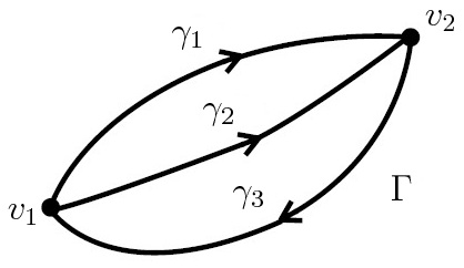
Figure 1: Closed graph $\Gamma$ with three links and two vertices. Link $\gamma_{k}$ carrying a charge $n_{k}$, charge conservation at vertex $v_{1}$ (or $v_{2}$) amounts to $-n_{1}-n_{2}+n_{3}=0$.

The vectors of ${\cal H}_{\rm Cyl}$ obeying the condition of gauge invariance span the non-separable “kinematical” Hilbert space ${\cal H}_{\rm kin}$ $\subset$ ${\cal H}_{\rm Cyl}$.

4.2 Physical Hilbert space

The last constraint to be imposed is the curvature constraint ${\cal C}_{2}$ in (3.15), whose quantum expression is $\hat{F}\left|{\Psi}\right\rangle=0$. Its general solution is given by a wave functional $\Psi[A]$ whose argument A is a connection with null curvature. It is sufficient to impose this condition on the basis vectors of ${\cal H}_{\rm kin}$ (charge networks), which will select the basis of the physical Hilbert space ${\cal H}_{\rm phys}$ $\subset$ ${\cal H}_{\rm kin}$.

The condition of null curvature means that, locally, there exists a scalar function ${\varphi}$ such that

$$A_{a}=\partial_{a}{\varphi}\,.$$ (4.4)

The rest of the discussion depends on the topology of the space sheet $\Sigma$.

Let us begin with the case where the topology of $\Sigma$ is that of $\mathbb{R}^{2}$. Then (4.4) holds globally, with the result that the holonomy associated to any link $\gamma$ with initial and final end points ${\boldsymbol{x}}_{\rm i}$ and ${\boldsymbol{x}}_{\rm f}$ takes the form

$$h_{\gamma}[A]=\exp({\varphi}({\boldsymbol{x}}_{\rm f})-{\varphi}({\boldsymbol{x}}_{\rm i}))\,.$$

Together with the fact that that the graph associated to any charge network $\left|{\Gamma,\vec{n}}\right\rangle$ is closed and that the charge conservation condition must hold at each vertex, one easily sees that its wave functional $\Psi_{\Gamma,\vec{n}}$ is equal to 1. In other words, the graph $\Gamma$ shrinks to a single point, and we are left with the sole vector $\left|{\emptyset}\right\rangle$. The physical Hilbert space is reduced to a trivial 1-dimensional space.

The next case is that with the topology of $\mathbb{R}^{2}\backslash\{O\}$, the 2-dimensional plane with one point $O$ suppressed. There are now two classes of closed graphs, those with $O$ inside and those with $O$ outside. Two examples of the former class are shown in Fig. 2.

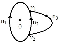
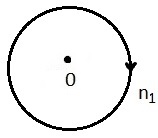
Figure 2: Two charge network graphs with the singular point O “inside”.

Applying the charge conservation condition as in the previous case shows that any charge network graph with the point $O$ “outside” reduces to a point with the resulting wave functional equal to 1, defining the empty state described by the vector $\left|{\emptyset}\right\rangle$. On the other hand, any charge network graph with the point $O$ “inside” is equivalent to a single loop $\gamma$ with $O$ inside, with the resulting wave functional equal to a unimodular complex number:

$$\langle{A|n}\rangle=\Psi_{n}[A]=\exp(inQ)\,,$$

with $n\in\mathbb{Z}$ the charge of the loop. The value of the “flux” $Q$, given by

$$\exp(iQ)=h_{C}[A]\,,$$

where $C$ is a closed positively oriented loop around the singular point $O$, is independent of the form and size of the loop, and the value of $n$ is computed using the charge conservation condition. Fig. 2 shows an example of two such equivalent graphs. The basis of the physical Hilbert space ${\cal H}_{\rm phys}$ then consists of the vectors $\left|{n}\right\rangle$, $n\in\mathbb{Z}$, with $\langle{n|n^{\prime}}\rangle=\delta_{nn^{\prime}}$. For $n=0$, one has $\left|{0}\right\rangle$ = $\left|{\emptyset}\right\rangle$, corresponding to the former class of graphs. One notes that the integer number $n$ can be interpreted as a winding number of the loop: to wind $n$ times around the singular point with charge 1, or to wind 1 time with charge $n$ yield the same wave functional.

The generalization to a plane with $N$ singular points, $\mathbb{R}^{2}\backslash\{O_{1},\cdots,O_{N}\}$, is straightforward. The basis vectors of ${\cal H}_{\rm phys}$ read $\left|{\vec{n}}\right\rangle$ = $\left|{n_{1},\cdots,n_{N}}\right\rangle$ where $n_{k}$ is the charge (or winding number) of a loop encircling the $k^{\rm th}$ singular point, all the other singular points remaining outside of it. The corresponding wave functional is explicitly given by

$$\langle{A|\vec{n}}\rangle=\Psi_{\vec{n}}[A]=\exp(i\sum_{k=1}^{N}n_{k}Q_{k})\,,$$ (4.5)

where $Q_{k}$ is the flux associated to the $k^{\rm th}$ singular point, defined by:

$$\exp(iQ_{k})=h_{C_{k}}[A]\,,$$ (4.6)

where

$$\begin{array}[]{l}C_{k}=\mbox{closed loop encircling positively one time the singular point}\ O_{k}\\ \phantom{C_{k}=}\mbox{ and leaving aside all the other ones.}\end{array}$$ (4.7)

The orthonormality relations are

$$\langle{n_{1},\cdots,n_{N}|n^{\prime}_{1},\cdots,n^{\prime}_{N^{\prime}}}\rangle=\delta_{NN^{\prime}}\prod_{k=1}^{N}\delta_{n_{k}n_{k}^{\prime}}\,.$$

${\cal H}_{\rm phys}$ is separable.

One remarks that diffeomorphism invariance, which in the classical theory is a consequence of its gauge invariances, is explicit in the quantum theory constructed here, once all constraints are fulfilled. Note that the states of the (non-separable) kinematical Hilbert space, which still do not obey the curvature constraint ${\cal C}_{2}$, are not diffeomorphism invariant since they depend on the location and form of the associated graphs.

4.3 Observables

It follows from the above discussion that no non-trivial observables do exist in the case of a trivial topology such as that of $\mathbb{R}^{2}$. On the other side, with a non-trivial topology such as that of $\mathbb{R}^{2}$ with $N$ singular points $O_{k}$, there is a a set of $N$ observables $\hat{L}_{k}$, $k=1,\cdots,N$, simultaneously diagonalized in the basis (4.5) of ${\cal H}_{\rm phys}$:

$$\hat{L}_{k}\left|{\vec{n}}\right\rangle=n_{k}\left|{\vec{n}}\right\rangle\,,\quad k=1,\cdots,N\,.$$ (4.8)

They are explicitly given by

$$\hat{L}_{k}={\displaystyle{\int}\!\!\!}_{\Sigma}d^{2}x\,X^{(k)}_{a}({\boldsymbol{x}})\hat{B}^{a}({\boldsymbol{x}})\,,$$

where $X^{(k)}_{a}$ is a closed 1-form ($dX^{(k)}=0$), such that its integral on a loop $C_{k}$ as defined by (4.7), takes the value $i/\hbar$, whereas its integral on a loop $C_{l}$ around another singular point $O_{l}$ vanishes. Explicitly:

$${\displaystyle{\int}\!\!\!}_{C_{k}}X^{(l)}={\displaystyle{\frac{i}{\hbar}}}\delta_{kl}\,,$$ (4.9)

the result depending only on the homotopy class of $C_{k}$. In a polar coordinate frame $(r,\theta)$ centred in $O_{k}$, a particular solution for the 1-form $X^{(k)}$ is given by $(A_{r}=0$ and $A_{\theta}=i/(2\pi\hbar)$. The result (4.8) follows from the expression (4.5) for the basis vector functionals, together with (4.6) and the differentiation formula (taking into account the support property of $X^{(k)}$)

$${\displaystyle{\int}\!\!\!}_{\Sigma}d^{2}x\,X^{(k)}_{a}({\boldsymbol{x}}){\displaystyle{\frac{\delta}{\delta A_{a}({\boldsymbol{x}})}}}h_{C_{k}}[A]=\left({\displaystyle{\int}\!\!\!}_{C_{k}}X\right)h_{C_{k}}[A]\,.$$

The operators $\hat{L}_{k}$ thus defined are obviously self-adjoint in ${\cal H}_{\rm phys}$, and form a complete commutative set of observables.

5 Conclusions

What we have shown, using the Dirac canonical scheme together with the LQG quantization procedure, is that the three-dimensional Abelian BF model minimally coupled to a scalar field obeying a $\sigma$-model type of constraint, has the same degrees of freedom as the pure BF model. These degrees of freedom are non-local, of purely topological nature, characterized by the topological nature of space. They are represented by a complete set of $N$ commuting observables $\hat{L}_{k}$ in the case of the space topology being that o $\mathbb{R}^{2}$ with $N$ points ommitted ($N$ “punctures”).

The generalization to a non-Abelian version is not straightforward and will be presented in a future work [15].

References

- [1] Gerard ’t Hooft and M.J.G. Veltman, “One loop divergencies in the theory of gravitation”, Ann. Inst. Henri Poincaré A20 (1974) 69. (CERN). 1974.
- [2] B.S. DeWitt,“Quantum Theory of Gravity. I, II and III”, ,Phys. Rev. 160 (1967) 1113, Phys. Rev. 162 (1967) 1195,1239; J.A. Wheeler, in Battelle Rencontres: 1967 Lectures in Mathematics and Physics, eds. C.M. DeWitt and J.A. Wheeler (1968), p. 242.
-
[3]
C. Rovelli, “Quantum Gravity”, Cambridge Monography
on Math. Physics (2004);
A. Ashtekar and J. Lewandowski, “Background independent quantum gravity:
A status report”, Class. Quantum Grav. 21 (2004) R53, [arXiv:gr-qc/0404018];
T. Thiemann, “Modern Canonical Quantum General Relativity”,
Cambridge Monographs on Mathematical Physics (2008);
M. Han, W. Huang and Y. Ma “Fundamental structure of loop quantum gravity”,
Int. J. Mod. Phys. D16 (2007) 1397, [arXiv:gr-qc/0509064]. -
[4]
P.A.M. Dirac, “Lectures on Quantum Mechanics”,
Dover, 2001;
M. Henneaux, C. Teitelboim, “Quantization of Gauge Systems”, Princeton University Press, 1994. - [5] A. Ashtekar, “Lectures on Non-perturbative Quantum gravity”, Notes prepared in collaboration with R. S. Tate, World Scientific, Singapore (1991).
-
[6]
J.F. Barbero, “Reality conditions and Ashtekar
variables: A Different perspective”, Phys. Rev. D51 (1995) 5507,
[arXiv: gr-qc/9410013];
Giorgio Immirzi, “Real and complex connections for canonical gravity”,
Class. Quantum Grav. 14 (1997) L177, [arXiv: gr-qc/9612030]. -
[7]
J.A. Zapata, “Continuum spin foam model for 3d gravity”,
J. Math. Phys. 43 (2002) 5612. -
[8]
A. Perez, “Spin foam models for quantum gravity”,
Class. Quantum Grav. 20 (2003) R43. -
[9]
A. Achucarro and P. K. Townsend,
“A Chern-Simons Action for Three-Dimensional anti-De Sitter
Supergravity Theories”,
Phys. Lett. B180 (1986) 89;
Edward Witten. “(2+1)-Dimensional Gravity as an Exactly Soluble System”, Nucl. Phys. B311 (1988) 46;
Hans-Jurgen Matschull, “On the relation between 2+1 Einstein gravity and Chern- Simons theory”, Class. Quantum Grav. 16 (1999) 2599. - [10] S. Carlip and J. Gegenberg, “Gravitating topological matter in 2+1 dimensions”, Phys. Rev. D44 (424) 1991.
- [11] S. Carlip, J. Gegenberg and R.B. Mann, “Black holes in three-dimensional topological gravity”, Phys. Rev. D51 (6854) 1995.
- [12] L. Freidel, R.B. Mann and E.M. Popescu, “Canonical analysis of the BCEA topological matter model coupled to gravitation in (2+1) dimensions”, Class. Quantum Grav. 22 (3363) 2005.
- [13] K. Noui, A. Perez, “Three dimensional loop quantum gravity: Physical scalar product and spin foam models”, Class. Quantum Grav. 22 (2005) 1739, [arXiv:0402110[gr-qc]].
- [14] D.C.M. Mendonça, “Quantização de Laços no Modelo BF em 2+1 dimensões”, Master’s Thesis Universidade Federal do Espírito Santo - UFES (2010);
- [15] Diego Mendonça and Olivier Piguet, work in progress.
-
[16]
D. Birmingham, M. Blau and M. Rakowski, G. Thompson,
“Topological field theory‘”, Phys. Rep. 209 (1991) 129;
J.C. Baez, “An introduction to spin foam models of quantum gravity and BF theory”, Lect. Notes Phys. 543:25-94 (2000).