Posmon spectrosopy of quantum state on a circle

Abstract

Developing the analysis of the distribution of the particle’s position-momentum dot product, the so-called posmom $\mathbf{x}\cdot\mathbf{p}$, to quantum states on a circular circle on two-dimensional Cartesian coordinates, we give its posmometry (introduced recently by Y. A. Bernard and P. M. W. Gill, Posmom: The Unobserved Observable, J. Phys. Chem. Lett. 1(2010)1254) for eigenstates of the free motion on the circle, i.e., $z$-axis component of the angular momentum. The posmom has two parity symmetries, specifically, invariant under two operations $m_{x}$ and $m_{y}$ representing mirror symmetry about $x$ and $y$ axis respectively. The complete eigenfunction set of the posmom is then four-valued and consists of four basic parts each of them is defined within a distinct quadrant of the circle. The results are not only potentially experimentally testable, but also reflect a fact that the embedding of the circle $S^{1}$ in two-dimensional flat space $R^{2}$ is physically reasonable.

I Introduction

Recently, Gill et al. introduce a new operator, the particle’s position-momentum dot product $\mathbf{x}\cdot\mathbf{p}$, or posmom as they called, and establish a posmometry (the distribution density of the posmom) for some atomic and molecular systems. posmometry1 ; posmometry2 The posmom operator in one of the Cartesian axes, say, $x$ axis $Q_{x}\equiv(xp_{x}+p_{x}x)/2$, is an essentially self-adjoint operator. winter ; milburn In Ref.[liu141, ], we developed this operator on the a two-dimensional spherical surface $S^{2}$ and successfully worked out its distribution densities for some molecular rotational states. In this Letter, we explore the posmometry of quantum states on a circle which frequently model the planar rigid rotor, molecular rotation constrained on a plane, etc..

As embedding $S^{1}$ in the two-dimensional flat space $R^{2}$, there are two operators $Q_{i}$ $(i=x,y)$ that are respectively defined along two Cartesian axes of coordinate respectively, which turn out to take following form,

$$Q_{i}=\frac{1}{2}\left(x_{i}p_{i}+p_{i}x_{i}\right),$$ (1)

where $\mathbf{x}=(r\cos\varphi,r\sin\varphi),\varphi\in(0,2\pi)$, and $p_{x}=i\hbar/r\left(\sin\varphi\partial_{\varphi}+\cos\varphi/2\right)$, $p_{y}=-i\hbar/r\left(\cos\varphi\partial_{\varphi}-\sin\varphi/2\right)$. In fact, the momenta $p_{x}$ and $p_{y}$ are special case of the the so-called geometric momentum $\mathbf{p}=-i\hbar(\nabla_{surf}+M\mathbf{n/}2)$ liu133 on an $N$-dimensional surface which is embedded in $N+1$ dimensional Euclidean space, where $\nabla_{surf}$ is the gradient operator on surface, and $M$ is the mean curvature and $\mathbf{n}$ is the normal vector. liu133 The explicit forms of $Q_{x}$ and $Q_{y}$ are,

$$Q_{x}=\frac{i\hbar}{2}(\sin 2\varphi\frac{\partial}{\partial\varphi}+\cos 2\varphi),\text{ }Q_{y}=-Q_{x}.$$ (2)

In the following section II, I will present the elementary properties of this operator. In section III, I will give the posmometry for eigenstates of the $z$-component angular momentum $L_{z}:\Phi_{m}\left(\varphi\right)=\exp(im\varphi)/\sqrt{2\pi}$, $m=0,\pm 1,\pm 2,...$. Final section VI is our conclusions.

II Elementary properties of the posmom operator

The following properties of the two posmom operators $Q_{i}$ $(i=1,2)$ are easily attainable.

i) Since the geometric momentum $\mathbf{p}$ describes the motion constrained on the surface $S^{1}$ and there is no motion along the normal direction $\mathbf{n}$, which in quantum mechanics is expressed by $\mathbf{x\cdot p+p\cdot x}\equiv 2(Q_{x}+Q_{y})=0$ while it is in classical mechanics expressed by $\mathbf{x\cdot p}=0$. This is why two operators $Q_{x}$ and $Q_{y}$ are linearly dependent, as shown in Eq. (2). So it suffices to study one of the them, and I will concentrate $Q_{x}$.

ii) The operator $Q_{x}$ has the reflection symmetry:

$$Q_{x}(\Theta\pm\varphi)=Q_{x}(\Theta+\varphi),\text{ }\Theta=0,\frac{\pi}{2},\pi,\frac{3\pi}{2}.$$ (3)

In other words, posmom $Q_{x}$ commutes with two parity operators $m_{x}$ and $m_{y}$ denoting two reflections about axes $x=0$, $y=0$ respectively, and we have,

$$\left[m_{x},Q_{x}\right]=\left[m_{y},Q_{x}\right]=0.$$ (4)

This mirror invariance is helpful in construction of the complete set of the eigenfunctions on the circle once the eigenfunctions of $Q_{x}$ in four quadrants $\varphi\in(0,\pi/2),$ $(\pi/2,\pi)$, $(\pi,3\pi/2)$ and $(3\pi/2,2\pi)$ are known, respectively.

iii) In the full circle $\varphi\in(0,2\pi)$, we have the solution to the eigenvalue problem $Q_{x}\xi_{\lambda}(\varphi)=\hbar\lambda\xi_{\lambda}(\varphi)$,

$$\xi_{\lambda}(\varphi)=\frac{1}{\sqrt{\pi}}\frac{1}{\sqrt{\left|\sin 2\varphi\right|}}\exp(-i\lambda\ln\left|\tan\varphi\right|)\text{, }\lambda\in(-\infty,\infty),$$ (5)

which is delta function normalized in any one of four quadrants, say in the first: $\int_{0}^{\pi/2}\xi_{\lambda^{\prime}}^{\ast}(\varphi)\xi_{\lambda}(\varphi)d\varphi=\delta(\lambda^{\prime}-\lambda)$. For convenience, we can use $\left|\xi_{\lambda}^{J}\right\rangle$ ($J=I,II,III,IV$) to denote the eigenfunctions defined within the $J$th quadrants of the circle respectively.

iv) Note that $\left|\xi_{\lambda}^{J}\right\rangle$ is not the simultaneous eigenfunction of operators $Q_{x}(\varphi)$, $m_{x}$ and $m_{y}$. The complete simultaneous eigenfunction set of operators $Q_{x}(\varphi)$, $m_{x}$ and $m_{y}$ is given by,

$$\left|\psi_{\lambda}^{xy}\right\rangle =\left(\left|\xi_{\lambda}^{I}\right\rangle+\left|\xi_{\lambda}^{II}\right\rangle+\left|\xi_{\lambda}^{III}\right\rangle+\left|\xi_{\lambda}^{VI}\right\rangle\right)/2,$$ (6a)

$$\left|\psi_{\lambda}^{\overline{x}\overline{y}}\right\rangle =\left(\left|\xi_{\lambda}^{I}\right\rangle-\left|\xi_{\lambda}^{II}\right\rangle+\left|\xi_{\lambda}^{III}\right\rangle-\left|\xi_{\lambda}^{VI}\right\rangle\right)/2,$$ (6b)

$$\left|\psi_{\lambda}^{\overline{x}y}\right\rangle =\left(\left|\xi_{\lambda}^{I}\right\rangle+\left|\xi_{\lambda}^{II}\right\rangle-\left|\xi_{\lambda}^{III}\right\rangle-\left|\xi_{\lambda}^{VI}\right\rangle\right)/2,$$ (6c)

$$\left|\psi_{\lambda}^{x\overline{y}}\right\rangle =\left(\left|\xi_{\lambda}^{I}\right\rangle-\left|\xi_{\lambda}^{II}\right\rangle-\left|\xi_{\lambda}^{III}\right\rangle+\left|\xi_{\lambda}^{VI}\right\rangle\right)/2,$$ (6d)

where $$x \overline{x} x$$ and indicate even and odd parity respectively about -axis, and so on,

$$m_{x}m_{y}\left|\psi_{\lambda}^{xy}\right\rangle =m_{y}\left|\psi_{\lambda}^{xy}\right\rangle=\left|\psi_{\lambda}^{xy}\right\rangle,m_{x}m_{y}\left|\psi_{\lambda}^{\overline{x}\overline{y}}\right\rangle=-m_{y}\left|\psi_{\lambda}^{\overline{x}\overline{y}}\right\rangle=\left|\psi_{\lambda}^{\overline{x}\overline{y}}\right\rangle,$$ (7a)

$$m_{x}m_{y}\left|\psi_{\lambda}^{\overline{x}y}\right\rangle =m_{x}\left|\psi_{\lambda}^{\overline{x}y}\right\rangle=-\left|\psi_{\lambda}^{\overline{x}y}\right\rangle,m_{x}m_{y}\left|\psi_{\lambda}^{x\overline{y}}\right\rangle=m_{y}\left|\psi_{\lambda}^{x\overline{y}}\right\rangle=-\left|\psi_{\lambda}^{x\overline{y}}\right\rangle.$$ (7b)

The orthonormality and completeness of the eigenfunction set (6a)-(6d) are satisfied. I.e., we have following two relations,

$$1,\text{ }\left\langle\psi_{\lambda^{\prime}}^{i^{\prime}j^{\prime}}\left|\psi_{\lambda}^{ij}\right\rangle\right.=\delta(\lambda^{\prime}-\lambda)\delta_{i^{\prime}i}\delta_{j^{\prime}j},$$ (8)

where $(i,j)$ standing for $x,y,\overline{x}$, and $\overline{y}$. For any state $\Phi\left(\varphi\right)$ on the circle, we have,

$$2,\text{ }\Phi\left(\varphi\right)=\int_{-\infty}^{\infty}\alpha\left(\lambda\right)\psi_{\lambda}^{xy}\left(\varphi\right)d\lambda+\int_{-\infty}^{\infty}\beta\left(\lambda\right)\psi_{\lambda}^{\overline{x}\overline{y}}\left(\varphi\right)d\lambda+\int_{-\infty}^{\infty}\mu\left(\lambda\right)\psi_{\lambda}^{\overline{x}y}\left(\varphi\right)d\lambda+\int_{-\infty}^{\infty}\upsilon\left(\lambda\right)\psi_{\lambda}^{x\overline{y}}\left(\varphi\right)d\lambda,$$ (9)

where, $\int\left(\left|\alpha\left(\lambda\right)\right|^{2}+\left|\beta\left(\lambda\right)\right|^{2}+\left|\mu\left(\lambda\right)\right|^{2}+\left|\upsilon\left(\lambda\right)\right|^{2}\right)d\lambda=1$. This normalization clearly states that for a given $\lambda$, the distribution density $p(\lambda)$ usually comes form four parts,

$$p(\lambda)=\left|\alpha\left(\lambda\right)\right|^{2}+\left|\beta\left(\lambda\right)\right|^{2}+\left|\mu\left(\lambda\right)\right|^{2}+\left|\upsilon\left(\lambda\right)\right|^{2}\text{.}$$ (10)

It means that for a given $\lambda$, the probability amplitude is from Eq. (9) a four-valued function,

$$\alpha\left(\lambda\right) =\int_{0}^{2\pi}\psi_{\lambda}^{xy\ast}\left(\varphi\right)\Phi\left(\varphi\right)d\varphi,\text{ }\beta\left(\lambda\right)=\int_{0}^{\pi/2}\psi_{\lambda}^{\overline{x}\overline{y}\ast}\left(\varphi\right)\Phi\left(\varphi\right)d\varphi,$$ (11a)

$$\mu\left(\lambda\right) =\int_{0}^{2\pi}\psi_{\lambda}^{\overline{x}y\ast}\left(\varphi\right)\Phi\left(\varphi\right)d\varphi,\text{ }\upsilon\left(\lambda\right)=\int_{0}^{\pi/2}\psi_{\lambda}^{x\overline{y}\ast}\left(\varphi\right)\Phi\left(\varphi\right)d\varphi.$$ (11b)

However, in the following section, we see that for the eigenstates $$\Phi_{m}\left(\varphi\right)=\exp(im\varphi)/\sqrt{2\pi} z L_{z}$$ of the -component angular momentum , the probability amplitude is in general triple-valued.

III Posmometry for eigenstates of the $z$-component angular momentum $L_{z}$

As is well known, the $z$-component angular momentum $L_{z}=-i\hbar\partial_{\varphi}$ has a complete set of eigenfunctions $\Phi_{m}\left(\varphi\right)=\exp(im\varphi)/\sqrt{2\pi}$ ($m=0$, $\pm 1$, $\pm 2$, …) that span a Hilbert space for analyzing any state on $S^{1}$. In general, we have,

$$\frac{1}{\sqrt{2\pi}}\exp(im\varphi)=\int_{0}^{2\pi}\alpha_{m}\left(\lambda\right)\psi_{\lambda}^{xy}d\lambda+\int_{0}^{2\pi}\beta_{m}\left(\lambda\right)\psi_{\lambda}^{\overline{x}\overline{y}}d\lambda+\int_{0}^{2\pi}\mu_{m}\left(\lambda\right)\psi_{\lambda}^{\overline{x}y}d\lambda+\int_{0}^{2\pi}\upsilon_{m}\left(\lambda\right)\psi_{\lambda}^{x\overline{y}}d\lambda$$

where the expansion coefficients $\alpha_{m}\left(\lambda\right)$, $\beta_{m}\left(\lambda\right)$, $\mu_{m}\left(\lambda\right)$ and $\upsilon_{m}\left(\lambda\right)$ are given by,

$$\alpha_{m}\left(\lambda\right) =\frac{1+(-1)^{m}}{2\pi\sqrt{2}}\left(I_{m}\left(\lambda\right)+\exp\left(\frac{im\pi}{2}\right)I_{m}\left(-\lambda\right)\right),$$ (12a)

$$\beta_{m}\left(\lambda\right) =\frac{1+(-1)^{m}}{2\pi\sqrt{2}}\left(I_{m}\left(\lambda\right)-\exp\left(\frac{im\pi}{2}\right)I_{m}\left(-\lambda\right)\right),$$ (12b)

$$\mu_{m}\left(\lambda\right) =\frac{1-(-1)^{m}}{2\pi\sqrt{2}}\left(I_{m}\left(\lambda\right)+\exp\left(\frac{im\pi}{2}\right)I_{m}\left(-\lambda\right)\right),$$ (12c)

$$\upsilon_{m}\left(\lambda\right) =\frac{1-(-1)^{m}}{2\pi\sqrt{2}}\left(I_{m}\left(\lambda\right)-\exp\left(\frac{im\pi}{2}\right)I_{m}\left(-\lambda\right)\right),$$ (12d)

with,

$$I_{m}\left(\lambda\right) =\int_{0}^{\pi/2}\frac{\exp(im\varphi)}{\sqrt{\sin 2\varphi}}\exp(i\lambda\ln\tan\varphi)d\varphi$$ (13)

$$= \left(\frac{1}{2}+\frac{i}{2}\right)e^{-\frac{\pi\lambda}{2}}\Gamma\left(\frac{m+1}{2}\right)\left\{f(\lambda,m)-i^{m+1}f^{\ast}(\lambda,m)\right\},$$ (14)

in which with $F(a,b;c;z)$ symbolizing the hypergeometric function,

$$f(\lambda,m)=\frac{\Gamma\left(\frac{1}{2}+i\lambda\right)}{\Gamma\left(\frac{m}{2}+1+i\lambda\right)}\,F\left(\frac{1}{2}+i\lambda,\frac{m+1}{2};\frac{m}{2}+1+i\lambda;-1\right).$$ (15)

Because of the eigenfunctions $\Phi_{m}\left(\varphi\right)$ can be decomposed into two parts according to mirror symmetry operators: $\exp(im\varphi)/\sqrt{2\pi}=\left\{\cos(m\varphi)+i\sin(m\varphi)\right\}/\sqrt{2\pi}$, it is for our purpose sufficient to study the eigenfunctions $\Phi_{m}\left(\varphi\right)$ with $m\succeq 0$. Evidently, for $m$ being a positive even number $m=2k$ ($k=1,2,3,...$), we obtain,

$$\alpha_{2k}\left(\lambda\right) =\frac{1}{\sqrt{2}\pi}\left(I_{2k}\left(\lambda\right)+\left(-1\right)^{k}I_{2k}\left(-\lambda\right)\right),$$ (16a)

$$\beta_{2k}\left(\lambda\right) =\frac{1}{\sqrt{2}\pi}\left(I_{2k}\left(\lambda\right)-\left(-1\right)^{k}I_{2k}\left(-\lambda\right)\right),$$ (16b)

$$\mu_{2k}\left(\lambda\right) =\upsilon_{2k}\left(\lambda\right)=0.$$ (16c)

For $$m m=2k+1 k=1,2,3,...$$ being a positive odd number (), we obtain,

$$\mu_{2k+1}\left(\lambda\right) =\frac{1}{\sqrt{2}\pi}\left(I_{2k+1}\left(\lambda\right)+i\left(-1\right)^{k}I_{2k+1}\left(-\lambda\right)\right),$$ (17a)

$$\upsilon_{2k+1}\left(\lambda\right) =\frac{1}{\sqrt{2}\pi}\left(I_{2k+1}\left(\lambda\right)-i\left(-1\right)^{k}I_{2k+1}\left(-\lambda\right)\right),$$ (17b)

$$\alpha_{2k+1}\left(\lambda\right) =\beta_{2k+1}\left(\lambda\right)=0.$$ (17c)

So, we see that the probability amplitude is in general triple-valued. Unfortunately, the expansion coefficients ($$\alpha \beta \mu \upsilon m=0 m m=0 m=2k$$, , , ), provided nontrivial, can not be all greatly simplified unless and being odd. For and , we have following relations,

$$\alpha_{0}\left(\lambda\right) =\frac{\left|\Gamma\left(1/4-i\lambda/2\right)\right|^{2}}{2\pi^{3/2}},\beta_{0}\left(\lambda\right)=0,$$ (18a)

$$\alpha_{2k}\left(\lambda\right) \neq\beta_{2k}\left(\lambda\right),$$ (18b)

where $$m=0 m \left|\mu_{2k+1}\left(\lambda\right)\right|^{2}=\left|\upsilon_{2k+1}\left(\lambda\right)\right|^{2} m=1,3,5$$ is the only case the probability amplitude of the posmom is double valued. For being odd we have , and for , we have explicitly,

$$\mu_{1}\left(\lambda\right) =\frac{i}{\sqrt{2}\left(\cosh(\pi\lambda/2)-i\sinh(\pi\lambda/2)\right)},\text{ }\upsilon_{1}\left(\lambda\right)=-i\text{ }\mu_{1}^{\ast}\left(\lambda\right),\text{ }p_{1}(\lambda)=\sec h(\lambda\pi),$$ (19a)

$$\mu_{3}\left(\lambda\right) =\frac{\sqrt{2}\lambda}{\cosh\left(\pi\lambda/2\right)-i\sinh\left(\pi\lambda/2\right)},\text{ }\upsilon_{3}\left(\lambda\right)=-i\text{ }\mu_{3}^{\ast}\left(\lambda\right),\text{ }p_{3}(\lambda)=4\lambda^{2}\sec h(\lambda\pi),$$ (19b)

$$\mu_{5}\left(\lambda\right) =\frac{-(1-4\lambda^{2})i}{2\sqrt{2}\left(\cosh\left(\pi\lambda/2\right)-i\sinh\left(\pi\lambda/2\right)\right)},\text{ }\upsilon_{5}\left(\lambda\right)=-i\text{ }\mu_{5}^{\ast}\left(\lambda\right),\text{ }p_{5}(\lambda)=\frac{1}{4}\left(1-4\lambda^{2}\right)^{2}\sec h(\lambda\pi).$$ (19c)

The probability distributions $p(\lambda)$ (10) for rotational states represented by $e^{im\varphi}/\sqrt{2\pi}$ with $m=0$ to $6,40,41$ are plotted in Fig. 1 ($m=0,2$), Fig. 2 ($m=4$), Fig. 3 ($m=6$), Fig. 4 ($m=1,3,5$), Fig. 6 ($m=40$) and Fig. 6 ($m=41$) respectively. On the whole, they are similar to the momentum distributions of stationary states for the one-dimensional simple harmonic oscillator. It is understandable from an examination of the free motion on the circle. In classical mechanics for the free motion with a frequency $\omega$, we have $x=r\cos(\omega t)$ and $p_{x}=-m\omega r\sin(\omega t)$ and therefore $xp_{x}=-(m\omega r^{2}/2)\sin(2\omega t)$. Then, in a classical state, the posmom $xp_{x}$ has a half period as $x$ or $p_{x}$ has. In classical limit, whenever $m$ being even or odd number, the eigenstate $e^{im\varphi}/\sqrt{2\pi}$ behaves like a simple harmonic oscillator as seen from the posmom.

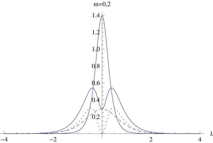
Figure 1: Distribution density of $Q_{x}$ for the ground state $1/\sqrt{2\pi})$ (solid line with highest peak near at $1.4$), and that for 2nd excited state $\exp{(2i\varphi)}/\sqrt{2\pi})$ which is the sum of $|\alpha(\lambda)|^{2}$ (dotted) and $|\beta(\lambda)|^{2}(\neq|\alpha(\lambda)|^{2})$ (dashed). Neither has a node.

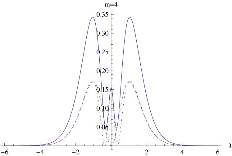
Figure 2: Distribution density of $Q_{x}$ for the 4th excited state $\exp{(4i\varphi)}/\sqrt{2\pi}$, which is the sum of $|\alpha(\lambda)|^{2}$ (dotted) and $|\beta(\lambda)|^{2}$ (dashed) but $|\alpha(\lambda)|^{2}$ and $|\beta(\lambda)|^{2}$ differ appreciately only near $\lambda=0$. This density has no node either.

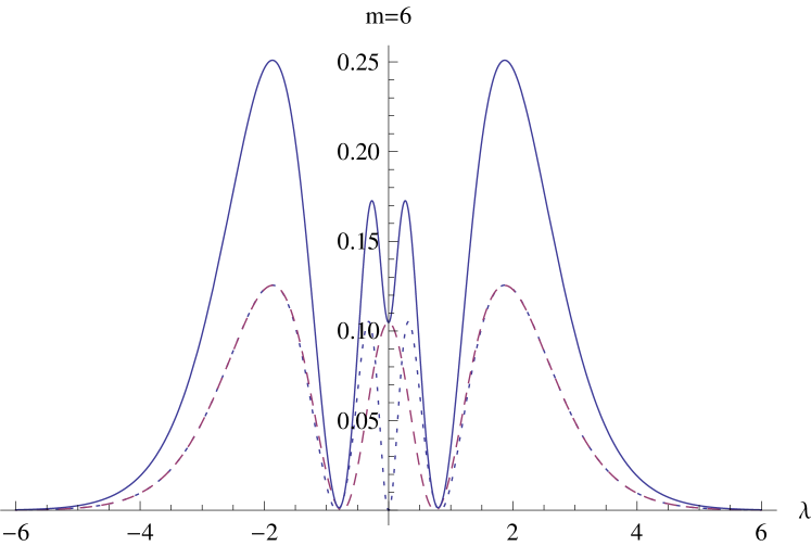
Figure 3: Distribution density of $Q_{x}$ for the 6th excited state $\exp{(6i\varphi)}/\sqrt{2\pi}$, which is the sum of $|\alpha(\lambda)|^{2}$ (dotted) and $|\beta(\lambda)|^{2}$ (dashed) and we see again that $|\alpha(\lambda)|^{2}$ and $|\beta(\lambda)|^{2}$ differ appreciately only near $\lambda=0$. The density exhibits no node but two minimum points over interval of finite $\lambda$ almost reach the zero.

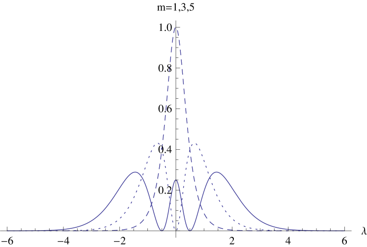
Figure 4: Distribution density of $Q_{x}$ for the 1st (dashed), 3rd (dotted) and 5th (solid) state $\exp{(im\varphi)}/\sqrt{2\pi})$, $(m=1,3,5)$. These distribution densities and the momentum distribution densities for the 0th, 1st and 2nd state of one-dimensional simple harmonic oscillator (not shown), are respectively similar.

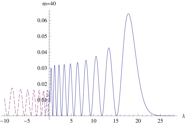
Figure 5: Distribution density of $Q_{x}$ for the 40th excited state $\exp{(40i\varphi)}/\sqrt{2\pi}$, which is symmetrical about $\lambda=0$ but only portion over the postive $\lambda$ is depicted. It is the sum of $|\alpha(\lambda)|^{2}$ (dotted) and $|\beta(\lambda)|^{2}$ (dashed) and they differ only near point $\lambda=0$; both symmetrical about $\lambda=0$ but half portions over the negative $\lambda$ are plotted. This distribution density has clearly $21$ peaks and $20$ minima in the interval of finite $|\lambda|<\infty$ but apparently $18$ nodes. To note that two minima near $\lambda=0$ appraoch closer as if they are a single one. We can infer that in the limit of large $m$ that is even, it is more and more similar to the distribution density for the $(m/2-1)$th state of one-dimensional simple harmonic oscillator.

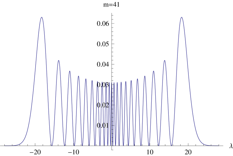
Figure 6: Distribution density of $Q_{x}$ for the 41th excited state $\exp{(41i\varphi)}/\sqrt{2\pi})$, which is the sum of two identical part $|\alpha(\lambda)|^{2}$ and $|\beta(\lambda)|^{2}$. The distribution density and the momentum distribution density for the $20$th excited state of one-dimensional simple harmonic oscillator (not shown), are almost the same. So, we can infer that in the limit of large $m$ that is odd, it becomes more and more similar to the distribution density for the $\{(m-1)/2\}$th state of one-dimensional simple harmonic oscillator.

IV Conclusions

The posmom offers a new way to understand the quantum motions, constrained or not. This study explores the posmom on a circular circle, and identify that the momentum in it is the geometric momentum that is recently proposed to properly describe of the momentum for the motions constrained on the curved surface. For construction of the complete basis, we need to resort to the mutual commutativity between posmom and parity operators, and then obtain the satisfactory bases each of them is in general four-valued. The posmometry of the eigenstates of the $z$-axis component of the angular momentum is worked out, and is found to be similar to the momentum distributions of stationary states for the one-dimensional simple harmonic oscillators. Then any states on the circle can thus go through the posmometry analysis. Once the posmometer is successfully designed and built up, the ground state of the planar rotation of some molecules, which can be easily prepared, can be visualized via the distribution of density of the posmom.

The present exploration riches not only our appreciation of the quantum dynamical behavior, but also our understanding of the fundamental aspect of the quantum mechanics.

References

(1) Y. A. Bernard, and P. M. W. Gill, New J. Phys.
11(2009)083015;
J. Phys. Chem. Lett. 1(2010)1254.
(2) P. M. W. Gill, Annu. Rep. Prog. Chem., Sect. C,
107(2011)229;
Y. A. Bernard, P. F. Loos, and P. M. W. Gill, Mol. Phys. 111(2013)2414.
(3) C. J. van Winter, Math. Phys. 39(1998)3600.
(4) J. Twamley, and G. J. Milburn, New J. Phys, 8(2006)328.