Field-ionization threshold and its induced ionization-window phenomenon for Rydberg atoms in a short single-cycle pulse

Abstract

We study the field-ionization threshold behavior when a Rydberg atom is ionized by a short single-cycle pulse field. Both hydrogen and sodium atoms are considered. The required threshold field amplitude is found to scale inversely with the binding energy when the pulse duration becomes shorter than the classical Rydberg period, and, thus, more weakly bound electrons require larger fields for ionization. This threshold scaling behavior is confirmed by both 3D classical trajectory Monte Carlo simulations and numerically solving the time-dependent Schrödinger equation. More surprisingly, the same scaling behavior in the short pulse limit is also followed by the ionization thresholds for much lower bound states, including the hydrogen ground state. An empirical formula is obtained from a simple model, and the dominant ionization mechanism is identified as a nonzero spatial displacement of the electron. This displacement ionization should be another important mechanism beyond the tunneling ionization and the multiphoton ionization. In addition, an “ionization window” is shown to exist for the ionization of Rydberg states, which may have potential applications to selectively modify and control the Rydberg-state population of atoms and molecules.

Studies on the ionization of atoms and molecules in an external field(s) have greatly broadened our knowledge of the microscopic electron dynamics, and also deepened our understanding on the correspondence between quantum and classical mechanicsexternal_field ; intense_field ; Gallagher ; Gutzwiller . Correspondingly, various ionization mechanisms have been identified for a diversity of interesting phenomena in different field configurations, such as closed-orbit theoryCOT , “simple-man’s” modelsimple_man00 ; simple_man01 ; simple_man02 , energy-level splitting and crossingsramp , successive Landau-Zener transitionmicro_wave , dynamical localizationlocalization , and also impulsive-kick ionization in a short half-cycle pulse (HCP) half00 ; half01 ; half_add . Recently, an intense single-cycle THz pulse has been applied to explore the ionization dynamics for low-lying Rydberg states of sodium atomsBob , where the field ionization threshold was found to scale as $n^{-3}$ ( $n$ denotes the principal quantum number), in contrast with all the threshold behaviors discovered beforeramp ; micro_wave ; localization ; half00 ; half01 . The threshold value is defined as the required field amplitude $F_{10\%}$ for $10\%$ ionization probability. Different threshold behavior corresponds to different ionization mechanism. This novel threshold behavior indicates that, when the pulse duration $t_{w}$ becomes comparable with (or even smaller than) the Rydberg period $T_{Ryd}=2\pi n^{3}$ (atomic units are used unless specified otherwise), the possible time effects imprinted by a short single-cycle pulse can be expected in the ionization dynamics.

In this paper, a new counterintuitive threshold scaling behavior is found in the short single-cycle pulse limit for both Rydberg states and much lower bound states, including the hydrogen ground state. The required threshold field amplitude is proportional to $(n/t_{w})^{2}$, which suggests that a stronger threshold field is required for higher Rydberg states. This threshold behavior is confirmed by comparing 3D classical trajectory Monte Carlo (CTMC) simulations with numerical results from directly solving the time-dependent Shrödinger (TDS) equation. It is further supported by a simple model where the dominant ionization mechanism is identified as a sudden and finite displacement of the electron in the short pulse duration. This displacement-ionization mechanism adds a new element in the strong-field ionization regime, which has received little attention before.

By combining with the adiabatic-ionization threshold in the low-frequency limitramp , it can be shown that there is an “ionization window” in the Rydberg series. The location of this “ionization window” can be adjusted by the pulse duration, and its width and height are dependent on the field strength. Since the generation of Rydberg states has been a routine, and the selective-field-ionization (SFI) technique has also been developed to identify the Rydberg-state population in atoms and moleculesGallagher , this “ionization window” phenomenon may have potential applications in future experiments to modify and control the Rydberg-state population.

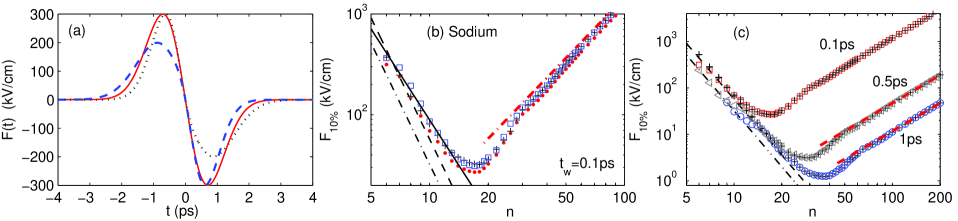
Figure 1: (Color online) (a) presents three typical single-cycle pulses. The solid, the dashed and the dotted curves represent, respectively, a “symmetric”, an “asymmetric” and an “inverted” field profiles given by Eq.(1). (b) displays the threshold behaviors for sodium with $t_{w}=0.1ps$. The red solid points, the open squares and the points indicated by “$+$” correspond respectively to a “symmetric” , an “asymmetric” and an “inverted” pulses. The bold dot-dashed line is from Eq.(4). The solid line indicates the $n^{-3}$ scaling behavior. (c) shows the threshold behaviors for both hydrogen and sodium with different $t_{w}$ values, where a “symmetric” pulse is applied. The blue circles, the gray triangles and the red squares display the thresholds for sodium with $t_{w}=1ps$, $t_{w}=0.5ps$ and $t_{w}=0.1ps$, respectively. The corresponding thresholds for hydrogen are denoted by “$+$”. The bold dashed lines are from Eq.(5). In both (b) and (c), the thin dashed and the thin dot-dashed lines (black online) represent the thresholds for hydrogen and sodium in the long pulse limit , respectively.

The single-cycle pulses in our calculations are constructed by the following vector potential,

$$A(t)=-\frac{F_{m}t_{w}}{C_{0}}e^{-\big{[}1\pm\frac{1}{a}\tanh\big{(}\frac{bt}{t_{w}}\big{)}\big{]}\big{(}\frac{t}{t_{w}}\big{)}^{2}},$$ (1)

where $F_{m}$ and $t_{w}$ are, respectively, the pulse maximum amplitude and the defined pulse duration; $a$ and $b$ are two adjustable parameters, and $C_{0}$ is dependent on the values of $a$ and $b$. Here, we first set $a=3$, $b=2$, and $C_{0}=1.016$. The signs“$+$” and “$-$” in the exponential factor correspond to an “asymmetric” pulse as in Ref.Bob and the “inverted” one, respectively. An amplitude-symmetric pulse is given by Eq.(1) with $b=0$ and $C_{0}=\sqrt{2}~{}e^{-1/2}$. Three typical pulses are plotted in Fig.1(a) with $t_{w}=1ps$. The total pulse length is about $4t_{w}$. For convenience, a related variable $\omega=\pi/(2t_{w})$ is defined to approximately denote the “field frequency”FT . The applied pulse field ($F(t)=-dA(t)/dt$) is assumed to be linearly polarized along the $z$-axis. A pure Coulomb potential is adopted for hydrogen. For sodium atoms, the following model potential is used,

$$V_{m}(r)=-\frac{Z^{*}(r)}{r}-\frac{\alpha}{2r^{4}}\Big{(}1-e^{-(\frac{r}{r_{c}})^{3}}\Big{)}^{2}$$ (2)

where $r$ is the radial coordinate of electron relative to the nucleus. $\alpha=0.9457$ and $r_{c}=0.7$. $Z^{*}(r)=1+10e^{-a_{1}r}+a_{2}re^{-a_{3}r}$ with $a_{1}=3.8538$, $a_{2}=11.0018$ and $a_{3}=3.0608$. Using 3D CTMC simulationsMC00 ; Topcu , the calculated thresholds $F_{10\%}$ (field amplitudes $F_{m}$ for $10\%$ ionization probability) are displayed in Fig.1(b)-(c) as a function of $n$, where $10^{5}$ trajectories are launched and the Rydberg electron is assumed to be initially in a $d$ state with the quantum angular momentum ($l=2$, $m=0$). The semiclassical angular momentum $l+0.5$ is used in the classical simulationsMC00 .

By applying the different pulses as those shown in Fig.1(a), the thresholds for sodium are displayed, respectively, in Fig.1(b) with $t_{w}=0.1ps$, which shows no qualitative change induced by the detailed pulse shape. The other similar results are presented in Fig.2, including those calculations with different initial angular momenta. We find that the threshold behaviors are not sensitive to the $l$ values, except that an effective quantum number $n^{*}$ should be adopted for sodium by considering the larger quantum defect for an $s$ state or a $p$ state induced by the ionic-core electrons. Therefore, the results presented in the following discussions are mainly for the atoms initially in a $d$ state, and a “symmetric” pulse is applied.

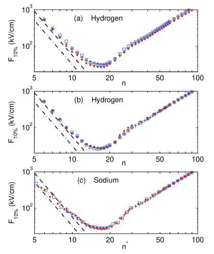
Figure 2: (Color online) Other similar results as those in Fig.1(b). (a) displays the threshold behaviors for hydrogen with different pulse profiles. The red solid points, the open squares and the points indicated by “$+$” correspond respectively to a “symmetric” , an “asymmetric” and an “inverted” pulses. (b) shows the threshold values for hydrogen Rydberg states with different angular-momentum quantum numbers, where a “symmetric” field profile is used. The red solid points, the open squares and the points labeled by “$+$” correspond respectively to the required threshold amplitudes for the Rydberg atom initially at an $s$ state, a $p$ state and a $d$ state. (c) is the same as (b) but for sodium, where an effective quantum number $n^{*}$ is used by including the quantum defects. In all the subplots (a)-(c), $t_{w}=0.1ps$. The dashed and the dot-dashed lines (black online) represent the thresholds for hydrogen and sodium in the long pulse limit , respectively.

For different field durations, a very similar threshold behavior is observed except a global shift between the different cases (see Fig.1(c)). This is not a surprise, because the classical Hamiltonian is invariant by defining two scaled variables ($Fn^{4}$, $t_{w}/n^{3}$) instead of the three quantities ($n$, $F$, $t_{w}$). As a result of this invariancescaling ; note , all the threshold curves in Fig.1 can be represented by one curve in the scaled space ($Fn^{4}$, $\omega n^{3}$) in Fig.3(a), where the displayed points are directly from the data in Fig.1(c) with $t_{w}=1ps$, and the results from other $t_{w}$ values are not displayed due to indistinguishability.

In the regime near the thin dashed lines in Fig.1 and Fig.3(a), where the pulse duration is much longer than $T_{Ryd}$, the threshold behaviors can be understood based on a picture of the energy-level splitting and crossingsramp . For much lower Rydberg states, the threshold for sodium is approximately equal to $n^{-4}/16$ indicated by the dot-dashed line, in contrast with that for hydrogen ($n^{-4}/9$) denoted by the thin dashed line. The corresponding ionization mechanism has been identified as an adiabatic over-the-barrier ionization, and the lower threshold for sodium is a signature of an avoided-crossing effect between energy levels due to the presence of ionic-core electrons. This adiabatic-ionization threshold supplies a fundamental principle for the SFI techniqueGallagher ; SFI . With the field varying faster, the threshold for sodium gradually deviates from $n^{-4}/16$ as a result of diabatic transition near the avoided crossings, and finally behaves in the same way as that for hydrogen. This effect can be observed clearly by comparing the threshold curves with $t_{w}=0.1ps$ and $t_{w}=1ps$ in Fig.1(c).

When the pulse duration becomes comparable with $T_{Ryd}$, the required threshold field strength can again deviate from the diabatic ionization threshold, and the time effect seems to be dominant in the ionization dynamics. For the initial stage, it has been observed to scale as $n^{-3}$ recentlyBob , as that indicated by the thin solid line in Fig.1(b). However, by going to the higher-lying Rydberg states where the pulse duration is shorter than $T_{Ryd}$, the required threshold will not continue to decrease. We find that a larger field amplitude is required for a more weakly-bound state. In the short pulse limit, the required threshold is proportional to $n^{2}$ as shown by the bold dashed line (red online) in Fig.1(c). Here, we would like to stress that, in the short pulse regime, there is no qualitative discrepancy between the threshold behaviors for sodium and hydrogen atoms.

To further confirm this counterintuitive behavior, a quantum calculation is made for hydrogen $15d$ state at different “scaled frequencies” ($\omega n^{3}$) by numerically solving the TDS equationTopcu ; TDS . We represent the wave function on a 2D space spanned by discrete radial points and an angular momentum basis, where a split operator method is used with a Crank-Nicolson approximation to propagate the wave function. For the radial part, a square-root-mesh scheme is used with a Numerov approximation. The results are displayed by the open squares in Fig.3(a), which agrees with the classical simulations.

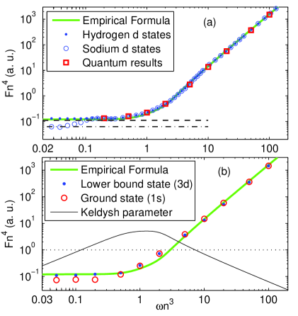
Figure 3: (Color online) Threshold scaling behaviors with (a) for Rydberg atoms and (b) for much lower bound states. $\omega$ is defined as $\pi/(2t_{w})$. A “symmetric” pulse is applied. In (a), the open and the solid circles are from Fig.1(c) for $t_{w}=1ps$. The quantum results for hydrogen $15d$ state at different scaled frequencies are shown by the red open squares. The dashed and the dot-dashed lines represent the thresholds for hydrogen and sodium in the low-frequency limit, respectively. In (b), the open and the solid circles correspond to the thresholds for hydrogen atoms initially in $1s$ state and $3d$ state, respectively. In both (a) and (b), the bold solid curve (green online) is from Eq.(6). The thin solid curve in (b) shows the variation of Keldysh parameter $\gamma$ associated with the bold solid line. The unity value of $\gamma$ is indicated by the dotted line.

In the short pulse limit, the observed threshold can be understood from a simple model. A similar idea was discussed in Ref.displacement . Consider a semiclassical atom with a quantized total energy $E_{n}=-\frac{1}{2n^{2}}$, an electron moves around the nucleus with $r_{n}=n^{2}$. Such a simple Bohr’s model is not fully correct for highly elliptical states, but, as a first approximation, it provides a reasonable estimation and also insight for the electron dynamics in an atombook . By interacting with a very short pulse field, the ionization can only occur during a very short fraction of one Rydberg period. The electron experiences a sudden displacement $\Delta r$, and its kinetic energy is assumed to be unchanged approximately during the short-time displacement. Following this simple assumption, the condition for ionization should be

$$E_{n}+\frac{1}{r_{n}}-\frac{1}{r_{n}+\Delta r}\geq 0~{},$$ (3)

which requires $\Delta r\geq n^{2}$. In a single-cycle pulse given by Eq.(1), it can be shown that a freely-motion electron gets no momentum transfer from the field, but has a finite displacement. For a “symmetric” pulse, $\Delta r=\sqrt{(\pi e)/2}\cdot F_{m}t_{w}^{2}$. Hence, the threshold field amplitude $F_{th}$ is

$$F_{th}=\sqrt{\frac{2}{\pi e}}\cdot\frac{n^{2}}{t_{w}^{2}}~{}.$$ (4)

Note the symbol ‘$e$’ on the right-hand side of Eq.(4) refers to the base of natural logarithms. The predicted threshold in Eq.(4) is displayed by the bold dot-dashed line in Fig.1(b), where a good agreement with the numerical results can be observed except for a small quantitative discrepancy. We attribute this small discrepancy to the rough approximations in estimating $r_{n}$ and $\Delta r$.

By slightly modifying the constant coefficient on the right-hand side of Eq.(4), a best fit can be obtained with the numerical results, and we arrive at

$$F_{th}=\frac{\pi}{8}\cdot\frac{n^{2}}{t_{w}^{2}}$$ (5)

which is shown by the bold dashed lines in Fig.1(c). By incorporating the experimental observationBob ($F_{10\%}\varpropto n^{-3}$) in the middle regime as that shown in Fig.1(b), we find that the threshold behavior can be described very well by the following empirical formula in the whole range from a long pulse limit to a short pulse limit,

$$Fn^{4}=\frac{1}{9}e^{-\Omega}+\frac{1}{10}{\Omega}^{\frac{1}{3}}e^{-({\Omega}-1)^{2}}+\frac{1}{2\pi}{\Omega}^{2}e^{-(1/{\Omega})}$$ (6)

where $\Omega=T_{Ryd}/4t_{w}$ ($=\omega n^{3}$) which can be considered as an approximate “scaled frequency”. The above empirical expression in Eq.(6) is a simple combination of the different threshold behaviors in the three scaled-frequency regimes (an exponential factor is used in each term on the right-hand side of Eq.(6) to turn on the corresponding threshold scaling relation in each regime): the first term corresponds to the hydrogen threshold ($F_{10\%}=1/(9n^{4})$) in the low-frequency limitramp ; the second term is from the recent observationBob ; and the last term comes from Eq.(5) directly, corresponding to the threshold behavior in the short pulse limit. The predicted threshold curves are shown by the bold solid lines in Fig.3.

The same threshold scaling behavior in the short pulse limit is also observed for much lower bound states. For hydrogen $3d$ and $1s$ states, respectively, the required thresholds at different scaled frequencies are displayed in Fig.3(b) from numerically solving the TDS equation. To estimate the Keldysh parameter $\gamma$ ($=\omega n^{3}/(Fn^{4})$) in Fig.3(b), Eq.(6) is used. The $\gamma$ value is often used to estimate the importance of tunneling-ionization Keldysh00 ; Keldysh01 ; Keldysh02 . In the low-frequency regime where $\gamma$ is comparable with (or smaller than) one, the threshold for the ground state is lower than that for the highly-excited states, as a result of the larger tunneling rate. However, in the short pulse limit, the ionization threshold for the ground state also follows the same scaling relation as that observed for Rydberg states, despite the much smaller $\gamma$ valuenote_add . This observation suggests that the above discussed displacement ionization is another important mechanism for the strong-field ionization in short laser pulses, beyond the tunneling ionization and the multi-photon ionizationsimple_man00 ; simple_man01 ; simple_man02 . We note that the signature of non-zero displacement effect has been discussed recently by Ivanov et al. using a multi-cycle extreme-ultraviolet pulseIvanov .

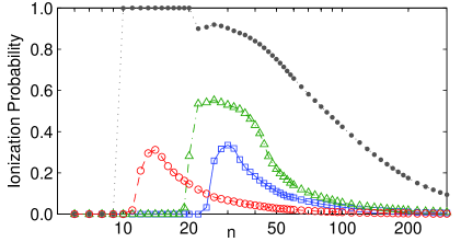
Figure 4: (Color online) “Ionization window” for Hydrogen Rydberg atoms initially in a $d$ state. The “symmetric” pulse in Fig.1(a) is used. The applied field amplitudes for the squares, the triangles, the open and the solid circles are $2.5kV/cm$, $5kV/cm$, $50kV/cm$ and $100kV/cm$, respectively. $t_{w}=0.1ps$ for the open circles, and $t_{w}=1ps$ for the others.

The proposed displacement-ionization mechanism has several fundamental differences from both the ionization dynamics induced by HCP(s) and the conventional field ionization. First of all, the dominant ionization induced by a short HCP occurs through a sudden impulsive kick, where a certain amount of momentum is transferred to an electronhalf00 ; half01 ; half_add , and which mainly changes the electron kinetic energy. In our present situation, however, displacement ionization is the dominant path, and the ionization occurs through a sudden spatial displacement of electron, which mainly changes the potential energy between electron and atomic nucleus. More importantly, the field ionization threshold in the short HCP limit has been proved to scale as $n^{-1}$half00 , which suggests that the more-weakly bound electron is still easier to be ionized. In contrast, the increasing threshold behavior ($n^{2}$) induced by the displacement ionization suggests that the more-deeply bound electron is easier to get ionized. The following “ionization window” phenomenon is one benefit from this displacement-ionization mechanism induced by a single-cycle pulse. What is more, HCP is a particularly-tailored pulse in practice. A real optical pulse must satisfy a zero net-force condition ($\int F(t)dt=0$) which is required by the Maxwell’s equations. Nevertheless, the net spatial displacement ($\int A(t)dt$) can be nonzero. Therefore, the single-cycle pulse is a natural limit of the fast-developing short-pulse generation technique. When the electric field of HCP or the present single-cycle pulse varies slowly enough, the situation will correspond to the conventional field ionizationramp , which we have discussed in the above context associated with Fig.1(c) where the differences between the threshold behavior in the low-frequency limit and that in the short-pulse limit can be observed clearly. It is these differences that make the following “ionization window” effect predictable and observable.

Based on the above observed threshold behaviors, an interesting phenomenon can be expected if a specific single-cycle pulse is applied to ionize a series of Rydberg states. It is shown in Fig.4 for hydrogen $d$ states by using 3D CTMC simulations. To avoid the possible influence of other $m$ states in the larger ionization probability, the initial $z$-component of classical angular momentum is restricted to be from $-0.5$ to $0.5$MC00 . For the low-lying Rydberg states where $t_{w}$ is much longer than $T_{Ryd}$, the adiabatic ionization is dominant, and the more deeply bound states cannot be ionized because $F_{th}\varpropto n^{-4}$. However, for the high-lying Rydberg states where $t_{w}$ is much shorter than $T_{Ryd}$, the displacement ionization is dominant, and the more weakly bound states can be hardly ionized since $F_{th}\varpropto n^{2}$. Consequently, an “ionization window” is formed by the different threshold scaling relations between the adiabatic-ionization regime and the displacement-ionization regime.

Only the Rydberg states falling in the “ionization window” are strongly ionized. The location of this “window” is determined by the pulse duration and can be estimated from Fig.1(c) and Eq.(6). Its width and height can be adjusted by the field amplitude. The width can also be estimated using Eq.(6). These features are demonstrated in Fig.4 by the squares, the open circles and the triangles, which supplies a possible application in future experiments as we discussed above. It is interesting to note that the ionization seems saturated suddenly for the Rydberg states with $n=10\thicksim 20$ in Fig.4 when $F_{m}=100kV/cm$. To understand this, we first note that the scaled frequency $\omega n^{3}=0.3$ for $n=20$ when $t_{w}=1ps$. For the Rydberg states with $n$ lower than $20$, the value of $\omega n^{3}$ is less than $0.3$, and the applied pulse falls in the low-frequency regime in Fig.4, where the time effect is much smaller, and the ionization probability can increase quickly once the applied field strength becomes slightly larger than the required threshold amplitude, which accounts for the saturated ionization in Fig.4.

In conclusion, inspired by a recent experiment on the ionization of sodium Rydberg atom by an intense single-cycle pulse Bob , we have investigated the threshold behaviors for both hydrogen and sodium atoms in a short single-cycle pulse field. Besides the newly reported threshold behaviorBob , the required threshold field amplitude was found to scale as $n^{2}$ in the short pulse limit. This result has been confirmed by both 3D CTMC simulations and numerically solving TDS equation. The ionization threshold for the hydrogen ground state also follows the same scaling behavior in the short pulse limit. The dominant ionization mechanism was identified as a sudden displacement of the electron by a short single-cycle pulse, and an empirical expression was also obtained. This displacement ionization is a new mechanism for the strong-field ionization of atoms and molecules, which holds important implications for the future experiments, especially with short laser pulses. Finally, an “ionization window” was predicted for the ionization of Rydberg states, which may have potential applications.

We thank Prof. C. H. Greene for the helpful discussions. This work was supported by the U.S. Department of Energy, Office of Science, Basic Energy Sciences, under Award number DE-SC0012193.

References

- (1) P. Schmelcher and W. Schweizer (Eds.), Atoms and Molecules in Strong External Fields, (Plenum Press, New York 1998).
- (2) T. Brabec (Ed.), Strong field laser physics, (Springer, New York 2008).
- (3) T. F. Gallagher, Rydberg Atoms, (Cambridge University Press, Cambridge, England, 1994), 1st ed..
- (4) M. C. Gutzwiller, Chaos in Classical and Quantum Mechanics, (Springer, New York, 1990).
- (5) M. L. Du and J. B. Delos, Phys. Rev. Lett. 58, 1731 (1987); D. Kleppner and J. B. Delos, Found. Phys. 31, 593 (2001) and references therein.
- (6) H. B. van Linden van den Heuvell and H. G. Muller, in Multiphoton Processes, edited by S. J. Smith and P. L. Knight (Cambridge University Press, Cambridge, England, 1988).
- (7) T. F. Gallagher, Phys. Rev. Lett. 61, 2304, (1988); E. S. Shuman, R. R. Jones, and T. F. Gallagher, Phys. Rev. Lett. 101, 263001, (2008).
- (8) P. B. Corkum, N. H. Burnett, and F. Brunel, Phys. Rev. Lett. 62, 1259, (1989); P. B. Corkum, Phys. Rev. Lett. 71, 1994, (1993).
- (9) T. W. Ducas, M. G. Littman, R. G. Freeman, and D. L. Kleppner, Phys. Rev. Lett. 35, 366 (1975); T. H. Jeys et al., Phys. Rev. Lett. 44, 390 (1980); J. L. Dexter and T. F. Gallagher, Phys. Rev. A 35, 1934 (1987). G. M. Lankhuijzen and L. D. Noordam, Adv. At. Mol. Opt. Phys. 38, 121 (1997) and the references therein.
- (10) P. Pillet, W. W. Smith, R. Kachru, N. H. Tran, and T. F. Gallagher, Phys. Rev. Lett. 50, 1042 (1983); P. Pillet, H. B. van Linden van den Heuvell, W. W. Smith, R. Kachru, N. H. Tran, and T. F. Gallagher, Phys. Rev. A 30, 280 (1984); L. Perotti, Phys. Rev. A 73, 053405 (2006).
- (11) S. Fishman, D. R. Grempel, and R. E. Prange, Phys. Rev. Lett. 49, 509 (1982); H. Maeda and T. F. Gallagher, Phys. Rev. Lett. 93, 193002 (2004); A. Schelle, D. Delande, and A. Buchleitner, Phys. Rev. Lett. 102, 183001 (2009).
- (12) R. R. Jones, D. You, and P. H. Bucksbaum, Phys. Rev. Lett. 70, 1236 (1993); C. O. Reinhold, M. Melles, and J. Burgdörfer, Phys. Rev. Lett. 70, 4026 (1993); M. T. Frey, F. B. Dunning, C. O. Reinhold, and J. Burgdörfer, Phys. Rev. A 53, 2929 (1996).
- (13) C. Raman, C. W. S. Conover, C. I. Sukenik, and P. H. Bucksbaum, Phys. Rev. Lett. 76, 2436 (1996); R. B. Vrijen, G. M. Lankhuijzen, and L. D. Noordam, Phys. Rev. Lett. 79, 617 (1997).
- (14) A. Emmanouilidou and T. Uzer, Phys. Rev. A 77, 063416 (2008); J. S. Briggs and D. Dimitrovski, New J. Phys. 10, 025013 (2008).
- (15) Sha Li and R. R. Jones, Phys. Rev. Lett. 112, 143006 (2014).
- (16) One can show that a fourier-transformed spectra of the “symmetric” pulse in Fig.1(a) has a peak at about .
- (17) F. Robicheaux, Phys. Rev. A 56, 3358(R) (1997).
- (18) T. Topçu and F. Robicheaux, J. Phys. B 40, 1925, (2007).
- (19) B. Kaulakys, V. Gontis, G. Hermann, and A. Scharmann, Phys. Lett. A 159, 261, (1991).
- (20) To get exactly the same results, the initial angular momentum also needs to be scaled as accordingly, but the influence of this angular-momentum term in the Hamiltonian is relatively small and is hardly to be observed clearly, especially for the Rydberg states.
- (21) F. Robicheaux, C. Wesdorp, and L. D. Noordam, Phys. Rev. A 62, 043404 (2000) and the references therein.
- (22) F. Robicheaux, J. Phys. B 45, 135007, (2012).
- (23) C. Wesdorp, F. Robicheaux, and L. D. Noordam, Phys. Rev. Lett. 87, 083001 (2001).
- (24) C. E. Burkhardt and J. J. Leventhal, Topics in Atomic Physics, (New York, Springer, 2006).
- (25) L. V. Keldysh, Sov. Phys. JETP 20, 1307 (1965).
- (26) V. S. Popov, Phys. Usp. 47, 855 (2004) and the references therein.
- (27) T. Topçu and F. Robicheaux, Phys. Rev. A 86, 053407, (2012).
- (28) There is a small contribution from tunneling ionization, which can decrease the corresponding threshold value slightly, but it can be hardly seen in Fig.3(b).
- (29) I. A. Ivanov, A. S. Kheifets, K. Bartschat, J. Emmons, S. M. Buczek, E. V. Gryzlova, and A. N. Grum-Grzhimailo, Phys. Rev. A 90, 043401, (2014).