Local tests of global entanglement
and a counterexample to the generalized area law

Abstract

We introduce a technique for applying quantum expanders in a distributed fashion, and use it to solve two basic questions: testing whether a bipartite quantum state shared by two parties is the maximally entangled state and disproving a generalized area law. In the process these two questions which appear completely unrelated turn out to be two sides of the same coin. Strikingly in both cases a constant amount of resources are used to verify a global property.

1 Introduction

In this paper we address two basic questions:

1. Can Alice and Bob test whether their joint state is maximally entangled while exchanging only a constant number of qubits? More precisely, Alice and Bob hold two halves of a quantum state $|\psi\rangle$ on a $D^{2}$-dimensional space for large $D$, and would like to check whether $|\psi\rangle$ is the maximally entangled state $|\phi_{D}\rangle=\frac{1}{\sqrt{D}}\sum_{x}|x\rangle|x\rangle$ or whether it is orthogonal to that state. The first entanglement tester is the hashing protocol of the influential 1996 paper by Bennett, DiVincenzo, Smolin and Wootters [9]; further results are summarized in table Table 1. Entanglement testing has found various applications, including entanglement distillation and error correction [9], state authentication [6] and bounding the communication capacities of bipartite unitary operators [18]. As can be seen from this table, all known protocols for this task require resources (communication, shared randomness or catalyst) which grow with $D$ [9, 6, 18].

2. Is there a counterexample to the generalized area law? A sweeping conjecture in condensed matter physics, and one of the most important open questions in quantum Hamiltonian complexity theory, is the so called “area law,” which asserts that ground states of quantum many body systems on a lattice have limited entanglement. Specifically, assume the system is described by a gapped local Hamiltonian $H=H_{1}+\ldots+H_{m}$, where each $H_{i}$ describes a local interaction between two neighboring particles of a lattice. The area law conjectures that for every subset $S$ of the particles, the entanglement entropy between $S$ and $\bar{S}$ for the ground state of $H$ is bounded by a constant times the size of the boundary of $S$. The area law, which has been proven for 1-D lattices [19] and is conjectured for higher degree lattices, is of central importance in condensed matter physics as it provides the basic reason to hope that ground states of gapped local Hamiltonians on lattices might have a (relatively) succinct classical description. The generalized area law (a folklore conjecture) transitions from this physically motivated phenomenon to a very clean and general graph theoretic formulation, where in place of edges of the lattice, the terms of the Hamiltonian correspond to edges of an arbitrary graph. The generalized area law then states that for any subset $S$ of vertices (particles), the entanglement entropy between $S$ and $\bar{S}$ for the ground state is bounded by some constant times the cut-set of $S$ (the number of edges leaving $S$).

We affirmatively answer both questions, based on a common technique that may be thought of as applying quantum expanders in a distributed fashion. Indeed these two questions which at first sight seem completely unrelated turn out to be two sides of the same coin.

reference	form of $|\psi\rangle$	communication required	other resources
[9]	$n$ EPR pairs	$O(n\log(1/\varepsilon))$	consumes only $O(\log(1/\varepsilon))$ EPR pairs
[6]	$n$ EPR pairs	$(2+o(1))\log(n/\varepsilon)$	$O(n/\log(n/\varepsilon))$ bits of shared randomness
[18]	$n$ EPR pairs	$O(\log(1/\varepsilon))$	$n/\varepsilon$ EPR pairs
this paper	$n$ EPR pairs	$O(\log(1/\varepsilon))$

Table 1: Comparison of different entanglement-testing protocols. When we say that communication $x$ is required, this means that we need to consume either $x$ qubits or, alternatively (by teleportation), $2x$ classical bits and $x$ EPR pairs. The exception is the first row, which uses classical communication to verify entanglement, and hence the entanglement cost is lower.

1.1 Main idea and results

The main ingredient in both proofs is the notion of quantum expanders, which we discuss further in Section 2. A quantum expander can be thought of as a collection of $d$ unitaries $U_{1},\ldots,U_{d}$, (think of $d$ as a constant) each acting on a (possibly large) dimension-$D$ Hilbert space. For any matrix $X$ on the $D$-dimensional Hilbert space, the operator associated with the expander, $\mathcal{E}(X)=\frac{1}{d}\sum_{i=1}^{d}U_{i}XU_{i}^{\dagger}$, has the unique eigenvalue 1 for the eigenvector $X=\mathbb{I}$ and next highest singular value $\lambda<1$. It thus shrinks any matrix orthogonal to the identity by a constant factor. The key to the results in the paper is an equivalent way to view quantum expanders, by considering their action on maximally entangled states. It is well known that for any $U$, $U\otimes U^{*}$ acting on the maximally entangled state $|\phi_{D}\rangle=\frac{1}{\sqrt{D}}\sum_{i=1}^{D}|i\rangle\otimes|i\rangle$ leaves it as is. Of course, this remains true even if $U$ is drawn uniformly at random from the set $U_{1},\ldots,U_{d}$ of the expander. Remarkably, even though quantum expanders use only a constant number $d$ of unitaries, they leave intact only the maximally entangled state, and cause all other states to shrink by at least a constant amount.

For the entanglement-testing problem, we use the above intuition to derive a communication protocol which uses only a constant number of qubits, and detects a maximally entangled state of arbitrary dimension. This is described in Section 3. The idea is to determine whether Alice and Bob share a state that is invariant under $U_{i}\otimes U_{i}^{*}$ for $i=1,\ldots,d$, or far from invariant; i.e. whether the shared state is $|\phi_{D}\rangle$ or something orthogonal. To achieve this with $O(1)$ communication, suppose Alice and Bob each had access to a joint register initialized with $1/\sqrt{d}\sum_{i=1}^{d}|i\rangle$. Each could then apply controlled operators from this register to their share of the state $|\psi\rangle$: Alice would apply a controlled $U_{i}$ and Bob a controlled $U_{i}^{*}$. This “shared register” model could more naturally be achieved by having Alice create the state and perform her controlled $U_{i}$ before sending the state to Bob, who then performs his controlled $U_{i}^{*}$. Bob should then test that the control state remained intact, which happens iff the original state of the $D$-dimensional registers was indeed the maximally entangled state. With only a little more algebra, this shows that for any $D$, $\epsilon>0$, there exists a protocol which uses $O(\log 1/\epsilon)$ qubits of communication, after which Bob always accepts if the shared state is $|\phi_{D}\rangle$. If the shared state is orthogonal to $|\phi_{D}\rangle$, he accepts with probability at most $\epsilon$. Moreover, if Alice and Bob do start with the maximally entangled state $|\phi_{D}\rangle$, the protocol does not damage the state.

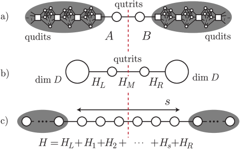
Figure 1: a) A counterexample to the generalized area law, consisting of a chain of complete graphs separated by the middle edge. The entropy across the cut is shown in Section 5 to grow as $\Omega\left(n^{c}\right)$, where $n$ is the total number of particles. b) A four-particle construction, analyzed in Section 4. c) Short-chain framework for proving 1-D area law, from [4].

For a counterexample to the generalized area law, we use the above intuition to exhibit a gapped local Hamiltonian acting on the graph featured in Figure 1 a), for which the entanglement entropy of the ground state across the middle cut is $\Omega(n^{c})$ for some $0<c<1$ (rather than $O(1)$ as predicted by the generalized area law). The core step in generating this example is the construction of a simpler system consisting of four particles on a line in Figure 1 b): two particles of dimension $d=3$ (qutrits) in the middle, and two particles of dimension $D$ at the two ends, with arbitrarily large $D$. The gapped Hamiltonian is of the form $H=H_{L}+H_{M}+H_{R}$, where $H_{L}$ acts between the left particle and the left qutrit, $H_{M}$ between the two qutrits, and $H_{R}$ between the right qutrit and the right particle. Crucially, the entanglement entropy of the ground state across the middle cut is $\Omega(\log D)$, as shown in Section 4. The idea here, like in the communication protocol, is to use the middle particles to synchronize the application of a quantum expander on the left and right sides. This requires only a single term of the Hamiltonian, acting on two $d$-dimensional particles.

Enforcing a large amount of entanglement (in the ground state) by the single constraint $H_{M}$ acting on a constant-dimensional system is a surprising quantum phenomenon. In the analogous probabilistic situation, consider a graph whise vertices are each associated with constant-dimensional variables, and whose edges are associated with classical constraints. Each constraint forbids some subset of the possible assignments to the variables at the two ends of the edge. This describes a constraint satisfaction problem (CSP). Now consider the uniform distribution over the set of all possible solutions to this set of constraints, namely all assignments that violate no constraint. It is easy to see that the middle constraint in the graph in Figure 1 a) can only enforce a convex combination of a constant number of product distributions .

This simple example of a four-particle system is already important within the context of proofs of the 1-D area law and prospects for extending those techniques to higher dimensions. The best current 1-D area law [4] works within a model very similar to our four-body Hamiltonian, except the middle link in [4] is extended into a finite chain of $s=\Omega(\log^{2}d/\epsilon)$ particles, each of dimension $d$ (see figure 1 c). This yields an area law bound of $S_{1-D}=O(\log^{3}(d)/\epsilon)$ across the middle cut. It was observed in [4] that any slight improvement in the exponent of $\log d$ would imply a non-trivial sub-volume law for 2-D systems. The crucial parameter in improving the result is the length of the middle chain; Our four-body Hamiltonian shows that in the extreme case of a length $1$ chain, no area law holds. Understanding the intermediate regime is thus an important open question.

Our four-particle example involves non-physical particles of arbitrarily large dimension. In Section 5 this example is converted to a counterexample to the generalized area law with bounded dimensional particles (albeit with unbounded degree of interaction). This is done by applying Kitaev’s circuit-to-Hamiltonian construction to implement the $U_{i}$, followed by an application of the strengthening gadgets of [13] (see Section 5 for details).

What is the connection between our two results? The above described Hamiltonian constructions are based on quantum expanders, just like our entanglement testers. In Section 6 we explore a deeper connection between very efficient communication protocols for EPR testing and violations of generalized area laws. We show that it is possible to derive a counterexample to the generalized area law, starting from a solution to the first problem (an EPR testing protocol with limited communication) and converting it using Kitaev’s circuit-to-Hamiltonian construction into a Hamiltonian violating the generalized area law. This, we believe, points at a fundamental link between the two seemingly unrelated topics. We discuss this and many other open questions and related work in Section 7.

Notation: For a matrix $X$, let $X^{*}$ be the entry-wise complex conjugate of $X$ and $X^{\dagger}$ the transpose of $X^{*}$. Define the Frobenius norm $|X|:=\sqrt{\operatorname{tr}X^{\dagger}X}$; the operator norm $\|X\|$ is the largest singular value of $X$.

2 Quantum Expanders

The key structural component to our results are quantum expanders. We will only make use here of expanders based on applying one out of $d$ unitaries at random (a more general definition using Kraus operators exists).

Definition 1.

The operator $\mathcal{E}:L(\mathbb{C}^{D})\rightarrow L(\mathbb{C}^{D})$ (here we use $L(\mathbb{C}^{D})$ to denote the set of linear operators on $\mathbb{C}^{D}$) is termed a $(D,d,\lambda)$ quantum expander if

• There are $d$ unitaries, $U_{1},U_{2},...,U_{d}$, such that $\mathcal{E}(X)=\frac{1}{d}\sum_{i=1}^{d}U_{i}XU_{i}^{\dagger}$.

• Interpreted as a linear map, $\mathcal{E}$ has second-largest singular value $\leq\lambda$.

Just as classical expanders may be thought of as constant-degree approximations to the complete graph, quantum expanders are constant-degree approximations to the application of unitaries drawn at random from the Haar measure.

By definition, the identity map $X=\mathbb{I}$ is the unique fixed point of $\mathcal{E}$. The second condition is equivalent to saying that for any $X$ with $\operatorname{tr}(X)=0$

$$|\mathcal{E}(X)|\leq\lambda|X|.$$ (1)

This interpretation suggests an alternate formulation where we think of each $X\in L(\mathbb{C}^{D})$ as a vector in $\mathbb{C}^{D}\otimes\mathbb{C}^{D}$ and the operator $\mathcal{E}$ then gets mapped to the operator $\hat{\mathcal{E}}=\frac{1}{d}\sum_{i=1}^{d}U_{i}\otimes U_{i}^{*}$. Then $\hat{\mathcal{E}}$ fixes the maximally entangled state $|\phi_{D}\rangle=\frac{1}{\sqrt{D}}\sum_{x\in[D]}|x\rangle|x\rangle$, and has second largest singular value $\lambda$.

Quantum expanders were introduced independently in [20] and [7] although many of the relevant ideas were implicit in [3]. In [21], it was proved that taking $U_{i}$ for $i\in\{1,...,d\}$ to be Haar uniform results in a “Ramanujan” expander with high probability; that is, $\lambda\approx 1/\sqrt{d}$. Since random unitaries cannot be constructed efficiently, other work [8, 17, 15, 24] gave efficient constructions, in which the unitaries can be applied by polynomial-size quantum circuits. Essentially all of these constructions achieve $\log(d)=O(\log 1/\lambda)$. For our communication protocols, we will need $d$ to be a variable (since the error depends on it); whereas for the area law counter example, we will take $d$ to be a small constant. In what follows we will assume for simplicity of exposition that $d=3$ is possible, although the smallest $d$ that has been verified is $d=8$ using [15].

Why are expanders relevant to our results? To understand the gap condition better, let us see why $|\phi_{D}\rangle$, the maximally entangled state on $\mathbb{C}^{D}\otimes\mathbb{C}^{D}$, is a $+1$ eigenvector. Observe that for any $D\times D$ matrix $X$, we have $(X\otimes I)|\phi_{D}\rangle=(I\otimes X^{T})|\phi_{D}\rangle$. Thus $\frac{1}{d}\sum_{i=1}^{d}(U_{i}\otimes U_{i}^{*})|\phi_{D}\rangle=\frac{1}{d}\sum_{i=1}^{d}(U_{i}U_{i}^{\dagger}\otimes I)|\phi_{D}\rangle=|\phi_{D}\rangle$. Since the second-largest singular value of $\hat{\mathcal{E}}$ is $\lambda$, then we have

$$\left\|\hat{\mathcal{E}}-|\phi_{D}\rangle\langle\phi_{D}|\right\|=\lambda.$$ (2)

Thus, $\hat{\mathcal{E}}$ gives an approximation of a projector onto $|\phi_{D}\rangle$ up to operator-norm error $\lambda$.

In the rest of our paper we will explore two settings in which this allows us to use resources proportional to $d$ (which we should think of as small) to force a state on $\mathbb{C}^{D}\otimes\mathbb{C}^{D}$ (with $D$ large) to be close to $|\phi_{D}\rangle$.

• In Section 3 we will show how $\log(d)$ qubits of communication can perform the projective measurement $\{|\phi_{D}\rangle\langle\phi_{D}|,I-|\phi_{D}\rangle\langle\phi_{D}|\}$ up to error $1/d^{\Omega(1)}$.

• In Section 4 we will show how interactions between a pair of constant-dimensional and a pair of two $D$-dimensional particles can have a ground state with maximal entanglement on the $D$-dimensional particles and a constant gap.

3 A communication protocol for certifying global entanglement

3.1 The EPR testing problem

As above, set $|\phi_{D}\rangle$ to be the maximally entangled state on $\mathbb{C}^{D}\otimes\mathbb{C}^{D}$. The EPR testing problem is to determine whether a given shared state $|\psi\rangle\in\mathbb{C}^{D}\otimes\mathbb{C}^{D}$ is equal to or orthogonal to $|\phi_{D}\rangle$. More precisely, two parties (Alice and Bob) would like to simulate the joint two-outcome POVM $\{|\phi_{D}\rangle\langle\phi_{D}|,\mathbb{I}-|\phi_{D}\rangle\langle\phi_{D}|\}$.

An $(D,\varepsilon)$ EPR tester is a communication protocol for performing a two-outcome measurement $\{M,\mathbb{I}-M\}$ such that $\|M-|\phi_{D}\rangle\langle\phi_{D}|\|\leq\varepsilon$.

In general EPR testers may differ in a variety of ways:

• If $M\geq|\phi_{D}\rangle\langle\phi_{D}|$ then we say the EPR tester has perfect completeness.

• The communication requirements and computational efficiency may vary.

• The protocol may be performed with quantum or classical communication. If quantum communication is used, then it is reasonable to assume that upon input $\rho$ the post-measurement state is $M^{1/2}\rho M^{1/2}/\operatorname{tr}[M\rho]$ or $(\mathbb{I}-M)^{1/2}\rho(\mathbb{I}-M)^{1/2}/\operatorname{tr}[(\mathbb{I}-M)\rho]$, depending on the outcome. If classical communication is used, we need to also consume some entanglement. We say that the test consumes $k$ EPR pairs if given an input of $n$ EPR pairs, it outputs at least $n-k$ EPR pairs (up to $\varepsilon$ error) when it reports success. There are no guarantees for orthogonal input states.

We are aware of three previous implementations of EPR testers (previously described in Table 1). Ref. [9] gave a $\left(2^{n},2^{-k}\right)$ EPR tester with perfect completeness that used a message of $O(nk)$ classical bits and consumed $k$ EPR pairs. This was improved by [6] to a $(2^{n},\frac{2n}{k(2^{k}+1)})$ EPR tester that sent $2k$ classical bits, consumed $k$ EPR pairs and used $\approx n/k$ bits of shared randomness. The paper [18] provides a protocol which uses only $\log 1/\varepsilon$ communication qubits, but with the assistance of an additional $n/\varepsilon$ trusted EPR pairs. Our protocol achieves a protocol with this amount of communication, without the need for any extra resources.

3.2 EPR testing with constant quantum communication

Our main result in this section is an EPR tester using only a constant amount of quantum communication that is independent of the dimension $D$.

Theorem 1.

For any $D$ and any $\varepsilon>0$ there exists a $(D,\varepsilon)$ EPR tester with perfect completeness using one-way communication from Alice to Bob. The protocol has several variants:

• Using $(2+o(1))\log(1/\varepsilon)$ qubits sent from Alice to Bob, but $\operatorname{poly}(D)$ run-time.

• Using $C\log(1/\varepsilon)$ qubits sent from Alice to Bob and $\operatorname{poly}\log(D)$ run-time for some universal constant $C>0$.

• Using either $(8+o(1))\log(1/\varepsilon)$ or $\approx\!4C\log(1/\varepsilon)$ classical bits sent from Alice to Bob (depending on whether computational efficiency is needed) and consuming the same number of EPR pairs.

• Using 2 bits of shared randomness and 1 qubit of communication, $\operatorname{poly}\log(D)$ run-time and achieving $\varepsilon=\frac{8+\sqrt{5}}{16}\leq 0.64$.

We remark that replacing the state $|\phi_{D}\rangle$ in Theorem 1 with a general entangled state can result in a much larger (and $D$-dependent) communication cost [18]. Thus we refer to the result as an EPR tester rather than a general entanglement tester.

One application of this result relates to the open question of whether entanglement helps quantum communication complexity. Classically, shared randomness does not significantly reduce communication complexity because large random strings can be replaced by pseudo-random strings that fool protocols[33]. This is called a blackbox reduction because it replaces the random input but does not change the protocol. Quantumly such blackbox reductions are ruled out by efficient entanglement-testing protocols, since they cannot be fooled by any low-entanglement state. A similar result is in [27] but their construction does not yield an EPR tester. See also [34] for a non-blackbox entanglement reduction that increases the communication cost by an exponential amount.

Proof of Theorem 1.

The main idea is to interpret the results of Section 2 as a way to test maximally entangled states. By Section 2 it suffices for Alice and Bob to implement a two-outcome measurement $\{M,\mathbb{I}-M\}$ on their shared state with $M=\hat{\mathcal{E}}$ for $\mathcal{E}$ a $(D,k,\sqrt{\varepsilon})$ expander. However, it is not immediately clear how to implement this measurement. To do this, we will use a trick that has been used in a variety of contexts (e.g. [5], [18] and Section 2.2.2 of [31]) and can be thought of as a variant of phase estimation. The protocol (depicted in Figure 3a) is as follows.

1. Alice and Bob initially share a state in registers $L,R$.

2. Alice prepares the $\log(d)$-qubit state $\frac{1}{\sqrt{d}}\sum_{i=1}^{d}|i\rangle$ in register $a$.

3. She performs $W=\sum_{i=1}^{d}|i\rangle\langle i|\otimes U_{i}$ on $a,L$.

4. She sends system $a$ to Bob.

5. Bob performs $W^{*}=\sum_{i=1}^{d}|i\rangle\langle i|\otimes U_{i}^{*}$ on $a,R$.

6. Bob does a two-outcome measurement on $a$, with the “accept” outcome corresponding to the state $\frac{1}{\sqrt{d}}\sum_{i=1}^{d}|i\rangle$ and the “reject” outcome corresponding to the orthogonal subspace.

If Alice and Bob start with the shared state $|\psi\rangle$, then step 5, their state is

$$\frac{1}{\sqrt{d}}\sum_{i=1}^{d}|i\rangle^{a}\otimes(U_{i}\otimes U_{i}^{*})|\psi\rangle^{LR}.$$ (3)

Step 6 then accepts with probability equal to the norm squared of $\frac{1}{d}\sum_{i=1}^{d}(U_{i}\otimes U_{i}^{*})|\psi\rangle=:M|\psi\rangle$ where we have defined

$$M=\frac{1}{d}\sum_{i=1}^{d}U_{i}\otimes U_{i}^{*}.$$ (4)

This results in the two-outcome measurement $\{M^{\dagger}M,I-M^{\dagger}M\}$. By Eq. (2), $M^{\dagger}M$ is $\varepsilon$ close to the desired measurement operator $|\phi_{D}\rangle\langle\phi_{D}|$.

The communication cost is $\log(d)$. If we do not care about computational efficiency, we can obtain $\varepsilon\approx 1/\sqrt{d}$ using random unitaries [21]. For a $\operatorname{poly}\log(d,D)$ run-time, we can iterate an efficient expander; e.g. applying the construction of [15] $k$ times yields $d=8^{k}$ and $\varepsilon\leq(2\sqrt{5}/8)^{k}$. To use classical bits instead, we first use the construction of [6] which uses $O(\log 1/\varepsilon)$ classical bits to verify $O(\log 1/\varepsilon)$ EPR pairs. Those EPR pairs are then used to teleport the qubits in the above protocol, which can therefore be applied to verify the rest of the EPR pairs.

For the last construction that uses two rbits and one qubit, we start with the quantum Margulis expander [15]. This consists of unitaries $U_{1},\ldots,U_{4},U_{5}=U_{1}^{\dagger},\ldots,U_{8}=U_{4}^{\dagger}$. The modified protocol is as follows. Let $r\in\{1,2,3,4\}$ be the value of the shared randomness. Run the above protocol with the pair of unitaries $\{I,U_{r}\}$. The resulting measurement operator, conditioned on $r$, is $M_{r}=\frac{I+U_{r}\otimes U_{r}^{*}}{2}$. Averaging over $r$ we obtain

$$M^{\dagger}M:=\frac{1}{4}\sum_{r=1}^{4}M_{r}^{\dagger}M_{r}=\frac{I+\frac{1}{8}\sum_{i=1}^{8}U_{i}\otimes U_{i}^{*}}{2}.$$

From the expansion properties proved in [15], we have that $\|M^{\dagger}M-|\phi_{D}\rangle\langle\phi_{D}|\|\leq\frac{1}{2}(1+\frac{2\sqrt{5}}{8})=\frac{8+\sqrt{5}}{16}$. ∎

To help prepare for the next sections, it is useful to view this test also in matrix form, as follows. If the initial state of the left/right registers was $|x\rangle_{L}|y\rangle_{R}$, after Alice’s operation, the state has to have the form

$$\frac{1}{\sqrt{d}}\sum_{i=1}^{d}|i\rangle(U_{i}|x\rangle_{L})|y\rangle_{R}.$$ (5)

After Bob gets the ancilla and performs his operation $W^{*}$, the state has to have the form

$$\frac{1}{\sqrt{d}}\sum_{i=1}^{d}|i\rangle\left(U_{i}|x\rangle_{L}\right)\left(U_{i}^{*}|y\rangle_{R}\right).$$ (6)

Let us represent the initial state $|\psi\rangle_{AB}=\sum_{k,\ell}x_{k,\ell}|k,\ell\rangle$ by a matrix $X$, such that $X_{k,\ell}=x_{k,\ell}$. We now rewrite the final state as a matrix with components $\beta_{(a,L),R}$:

$$\beta=\frac{1}{\sqrt{d}}\left[\begin{array}[]{c}U_{1}XU_{1}^{\dagger}\\ U_{2}XU_{2}^{\dagger}\\ \vdots\end{array}\right].$$ (10)

Passing the final test now means that

$$U_{i}XU_{i}^{\dagger}=U_{j}XU_{j}^{\dagger},\quad\forall i,j,$$ (11)

which is possible (if we have a quantum expander) only for $X=\mathbb{I}$. This means the initial state was $|\psi\rangle_{LR}=|\phi_{D}\rangle$, and that the final state is $\left(\frac{1}{\sqrt{d}}\sum_{i=1}^{d}|i\rangle_{a}\right)\otimes|\phi_{D}\rangle$.

4 A counterexample to the generalized area law

In this Section we present our second result: a Hamiltonian with a small “bridge” term connecting two large halves of a system. Strikingly, this single-link bridge of constant dimensions has a large influence on the entanglement entropy between the two parts of the system, in the ground state.

Figure 2: A single-link chain with side operators $L$ and $R$.

4.1 Background about local Hamiltonians

We consider Hamiltonians on finite-size spin systems, where each term in the Hamiltonian is a bounded-strength interaction between a bounded number of spins; in fact our constructions will involve only pairwise interactions. Unlike many physical systems, we do not require spatial locality but allow interactions between any pair of spins. We will also consider systems in which individual spin dimension $d_{i}$ can be large.

A quantum state on $n$ particles, of dimensions $d_{1},..,d_{n}$ respectively, is a unit vector in $\mathcal{H}:=\mathbb{C}^{d_{1}}\otimes\dots\otimes\mathbb{C}^{d_{n}}$. A Hamiltonian $H$ is a Hermitian matrix acting on $\mathcal{H}$. A $k$-local Hamiltonian can be written as $H=\sum_{i=1}^{m}H_{i}$ where each $H_{i}$ acts nontrivially on at most $k$ particles. Conventionally, each $\|H_{i}\|\leq 1$. If the $H_{i}$’s are all diagonal, $H$ is equivalent to a classical constraint satisfaction problem; in general the $H_{i}$ may not always be diagonal or even commute. The eigenvector of $H$ with the smallest eigenvalue is called the ground state. We say that a Hamiltonian is frustration free if the ground state of $H$ is also the eigenvector with lowest eigenvalue for each $H_{i}$; otherwise we call $H$ frustrated.

If the eigenvalues of $\mathcal{H}$ are $E_{0}\leq E_{1}\leq\cdots\leq E_{D-1}$ then the gap of $H$ is defined to be $E_{1}-E_{0}$. When $H$ belongs to a family of Hamiltonians indexed by $n$, we say this family is gapped if the gap of each $H$ is lower-bounded by a constant independent of $n$. (Otherwise the family is said to be gapless.) Often we identify $H$ with the family of Hamiltonians, and simply say that $H$ itself is gapped or gapless.

4.2 Construction of the Hamiltonian

Let the system $W$ consist of two qutrits ($\sigma_{1}$ and $\sigma_{2}$) and two high dimensional systems ($\Sigma_{L}$ and $\Sigma_{R}$):

$$W=\Sigma_{L}\otimes\sigma_{1}\otimes\sigma_{2}\otimes\Sigma_{R}=C^{D}\otimes C^{3}\otimes C^{3}\otimes C^{D}.$$

We design a gapped Hamiltonian $H=H_{L}+H_{M}+H_{R}$, where $H_{L}$ (left) $H_{M}$ (middle) and $H_{R}$ (right) are projectors acting on $\Sigma_{L}\otimes\sigma_{1}$, $\sigma_{1}\otimes\sigma_{2}$ and $\sigma_{2}\otimes\Sigma_{R}$, respectively, that defies the area law through the cut $\Sigma_{L}\otimes\sigma_{1}\,\mid\,\sigma_{2}\otimes\Sigma_{R}$. For convenience we write all elements of $W$ in the form

$$\sum_{i,j\in[3]}|\psi_{i,j}\rangle|i\rangle|j\rangle,$$

where $\psi_{i,j}\in\Sigma_{L}\otimes\Sigma_{R}$, and $\sum_{i,j\in[3]}|\psi_{i,j}|^{2}=1$. If we fix a basis in $\Sigma_{L}$ and $\Sigma_{R}$, respectively, we can think of $\psi_{i,j}$ for every $i,j\in[3]$ as $D\times D$ matrices. Our construction will rely on quantum expanders using $D\times D$ unitary matrices with $U_{1}=I$, and $U_{2}$ and $U_{3}$ such that for any $D\times D$ matrix $X$ with $|X|^{2}=\operatorname{tr}(XX^{\dagger})=1$, $\operatorname{tr}(X)=0$ we have:

$$|\mathcal{E}(X)|=\frac{1}{3}|X+U_{2}XU_{2}^{\dagger}+U_{3}XU_{3}^{\dagger}|\leq(1-c),$$ (12)

where $c:=1-\lambda>0$ is a fixed constant, independent of $D$. Equation (12) and the triangle inequality imply that for any $D\times D$ matrix $X$ with $|X|=1$, $\operatorname{tr}(X)=0$:

$$|U_{2}XU_{2}^{\dagger}-X|+|U_{3}XU_{3}^{\dagger}-X|\geq 3c$$ (13)

We now define projectors $H_{L}$, $H_{R}$ and $H_{M}$ via their zero subspaces ${\cal L}$, ${\cal R}$ and ${\cal M}$. We describe these subspaces by writing states of $W$ in the block matrix form

$$\left(\begin{array}[]{lll}\psi_{1,1}&\psi_{1,2}&\psi_{1,3}\\ \psi_{2,1}&\psi_{2,2}&\psi_{2,3}\\ \psi_{3,1}&\psi_{3,2}&\psi_{3,3}\\ \end{array}\right).$$

Note that our way to present a (pure) state of $W$ is unlike the density matrix presentation, and it is only meaningful, because $W$ is a tensor product of four components. The above matrix form (of a vector) is simply a convenient way of rendering the $(3D)^{2}$ coordinates of a state in $W$. In this presentation ${\cal L}$, ${\cal R}$ and ${\cal M}$ have convenient expressions. ${\cal L}$ is the set of states of the form

$$\left(\begin{array}[]{rrr}\psi_{1,1}&\psi_{1,2}&\psi_{1,3}\\ U_{2}\psi_{1,1}&U_{2}\psi_{1,2}&U_{2}\psi_{1,3}\\ U_{3}\psi_{1,1}&U_{3}\psi_{1,2}&U_{3}\psi_{1,3}\\ \end{array}\right),$$

where $\psi_{1,1}$, $\psi_{1,2}$ and $\psi_{1,3}$ are arbitrary. ${\cal R}$ is the set of states of the form

$$\left(\begin{array}[]{rrr}\psi_{1,1}&\psi_{1,1}U_{2}&\psi_{1,1}U_{3}\\ \psi_{2,1}&\psi_{2,1}U_{2}&\psi_{2,1}U_{3}\\ \psi_{3,1}&\psi_{3,1}U_{2}&\psi_{3,1}U_{3}\\ \end{array}\right),$$

where $\psi_{1,1}$, $\psi_{2,1}$ and $\psi_{3,1}$ are arbitrary. ${\cal M}$ is the set of states of the form

$$\left(\begin{array}[]{lll}\psi_{1,1}&X&Y\\ X&\psi_{2,2}&\psi_{2,3}\\ Y&\psi_{3,2}&\psi_{3,3}\\ \end{array}\right),\hskip 36.135pt$$

where $X$, $Y$ and the remaining $\psi_{i,j}$’s are arbitrary. It is easy to check that $H_{L},H_{M},H_{R}$ are indeed local. For instance ${\cal M}$ is a tensor product of $\Sigma_{L}\otimes\Sigma_{R}$ with the subspace $S$ of $\sigma_{1}\otimes\sigma_{2}$ that equates the coefficients of $|1\rangle|2\rangle$ and $|2\rangle|1\rangle$ and also the coefficients of $|1\rangle|3\rangle$ and $|3\rangle|1\rangle$. Explicitly

$$H_{L} :=\mathbb{I}-\frac{1}{3}\sum_{i,i^{\prime}=1}^{3}U_{i}U_{i^{\prime}}^{\dagger}\otimes|i\rangle\langle i|^{\prime},$$ (14a)

$$H_{R} :=\mathbb{I}-\frac{1}{3}\sum_{j,j^{\prime}=1}^{3}|j\rangle\langle j|^{\prime}\otimes\left(U_{j}U_{j^{\prime}}^{\dagger}\right)^{T},$$ (14b)

$$H_{M} :=\frac{(|12\rangle-|21\rangle)(\langle 12|-\langle 21|)}{2}+\frac{(|13\rangle-|31\rangle)(\langle 13|-\langle 31|)}{2}.$$ (14c)

4.3 The ground state is highly entangled

Lemma 2.

The unique normalized ground state $|G\rangle$ of $H=H_{L}+H_{R}+H_{M}=(\mathbb{I}-\Pi_{\cal L})+(\mathbb{I}-\Pi_{\cal R})+(\mathbb{I}-\Pi_{\cal M})$ written out as a matrix is

$$G=\frac{1}{3\sqrt{D}}\left(\begin{array}[]{lll}I&U_{2}&U_{3}\\ U_{2}&U_{2}^{2}&U_{2}U_{3}\\ U_{3}&U_{3}U_{2}&U_{3}^{2}\\ \end{array}\right).$$

It satisfies $H|G\rangle=H_{L}|G\rangle=H_{M}|G\rangle=H_{R}|G\rangle=0$.

Proof.

Equation (13) guarantees that $I$ is the only $D\times D$ matrix that commutes with both $U_{2}$ and $U_{3}$. From this together with the above forms of ${\cal L},{\cal R}$ and ${\cal M}$, it follows that $|G\rangle$ is the only normalized state vector in ${\cal L}\cap{\cal R}\cap{\cal M}$. ∎

Lemma 3.

The entanglement entropy of $|G\rangle$ along the $\Sigma_{L}\otimes\sigma_{1}\,\mid\,\sigma_{2}\otimes\Sigma_{R}$ cut is $\log_{2}D$.

Proof.

Let $|Z\rangle$ be any state on our-four particle system, and let $Z$ be its matrix notation. By a direct calculation, the reduced density matrix of $|Z\rangle$ on the $\Sigma_{L}\otimes\sigma_{1}$ systems is exactly $ZZ^{\dagger}$. Since $G=\frac{1}{3\sqrt{D}}\sum_{i,j=1}^{3}U_{i}U_{j}\otimes|i\rangle\langle j|$ (letting $U_{1}:=\mathbb{I}$), we have that for the ground state $|G\rangle$ the reduced density matrix

$$GG^{\dagger}=\frac{1}{3D}\sum_{i,i^{\prime}=1}^{3}U_{i}U_{i^{\prime}}^{\dagger}\otimes|i\rangle\langle i^{\prime}|.$$ (15)

To diagonalize $GG^{\dagger}$, let $W:=\sum_{i=1}^{3}U_{i}\otimes|i\rangle\langle i|$. Then

$$W^{\dagger}(GG^{\dagger})W=\frac{\mathbb{I}}{D}\otimes\frac{1}{3}\sum_{i,i^{\prime}=1}^{3}|i\rangle\langle i^{\prime}|,$$ (16)

which has $D$ eigenvalues equal to $1/D$. ∎

4.4 The Hamiltonian is gapped

Lemma 4.

Denote the energy gap above the ground space for the Hamiltonian $H=H_{L}+H_{M}+H_{R}$ by $\Delta$. Then $\Delta\geq c/4$ with $c$ defined in (12).

First we state a Lemma about the spectrum of the sum of two projectors.

Lemma 5.

Let $P_{1},P_{2}$ be projectors onto subspaces $V_{1},V_{2}$. Let

$$\mu:=\min\{\langle\psi|P_{2}|\psi\rangle:|\psi\rangle\in V_{1},\langle\psi|\psi\rangle=1\}=\lambda_{\min}(P_{1}P_{2}P_{1}).$$ (17)

Then the minimum eigenvalue of $\mathbb{I}-P_{1}+P_{2}$ is $1-\sqrt{1-\mu}\geq\mu/2$.

Proof.

By Jordan’s Lemma [28], it suffices to consider the case when

$$P_{1}=\begin{pmatrix}1&0\\ 0&0\end{pmatrix}\qquad\text{and}\qquad P_{2}=\begin{pmatrix}\mu&\sqrt{\mu(1-\mu)}\\ \sqrt{\mu(1-\mu)}&1-\mu\end{pmatrix}$$ (18)

In this case $P_{1}+P_{2}=I-(1-\mu)\sigma_{z}+\sqrt{\mu(1-\mu)}\sigma_{x}$ which has eigenvalues $1\pm\sqrt{1-\mu}$. ∎

Proof of Lemma 4.

Let $V_{LR}$ be the ground space of $H_{L}+H_{R}$ and let $\tilde{V}_{LR}$ be the subspace of $V_{LR}$ that is orthogonal to $|G\rangle$. Let $P_{LR},\tilde{P}_{LR}$ be the corresponding projectors and observe that

$$H_{L}+H_{R}\geq\mathbb{I}-P_{LR}\qquad\text{and}\qquad H_{L}+H_{R}+|G\rangle\langle G|\geq\mathbb{I}-\tilde{P}_{LR}.$$ (19)

Let $|\psi\rangle\in\tilde{V}_{LR}$ be a unit vector. Since $|\psi\rangle\in V_{LR}$, we can write it in matrix form as

$$|\psi\rangle=\left(\begin{array}[]{rrr}X&XU_{2}&XU_{3}\\ U_{2}X&U_{2}XU_{2}&U_{2}XU_{3}\\ U_{3}X&U_{3}XU_{2}&U_{3}XU_{3}\\ \end{array}\right).$$ (23)

Since $\langle G|\psi\rangle=0$ we additionally have $\operatorname{tr}[X]=0$. From normalization we have $|X|=1/3$. Now we calculate

$$\mu:=\langle\psi|H_{M}|\psi\rangle=\frac{|XU_{2}-U_{2}X|+|XU_{3}-U_{3}X|}{2}\stackrel{{\scriptstyle(\ref{eq:qexp2})}}{{\geq}}\frac{|X|}{2}3c=\frac{c}{2}$$ (24)

Setting $P_{1}=\tilde{P}_{LR}$ and $P_{2}=H_{M}$ we can now apply Lemma 5 and find that the minimum eigenvalue of $(\mathbb{I}-\tilde{P}_{LR})+H_{M}$ is $\geq c/4$. Finally, the second-smallest eigenvalue of $H_{L}+H_{M}+H_{R}$ is the minimum of $\langle\psi|H_{L}+H_{M}+H_{R}|\psi\rangle$ over all unit vectors $|\psi\rangle$ satisfying $\langle\psi|G\rangle=0$. For such a vector we have

$$\langle\psi|H_{L}+H_{M}+H_{R}|\psi\rangle=\langle\psi|(H_{L}+H_{M}+H_{R}+|G\rangle\langle G|)|\psi\rangle\geq\langle\psi|\mathbb{I}-\tilde{P}_{LR}+H_{M}|\psi\rangle\geq\frac{c}{4}$$ (25)

Combined with Lemma 2 this shows that the gap is $\geq c/4$. ∎

5 The abstract Hamiltonian can be implemented locally

The Hamiltonian construction in Section 4 has very interesting properties (a unique, very entangled ground state and a constant gap), but the $H_{L}$ and $H_{R}$ terms act on particles of arbitrary dimension. Alternatively, we can think of them as being nonlocal Hamiltonians for a system of qubits. We now wish to decompose them into local terms, acting on particles of dimension $O(1)$, while retaining their desirable properties. This is done in two steps: we first construct a Hamiltonian $H^{\prime}_{LMR}$ with the desired properties except the interactions are of polynomial strength, and then we correct this unphysical assumption and derive our final Hamiltonian $H^{\text{gadget}}_{LMR}$.

We start by showing in Subsection 5.1 that $H_{L}$ can be made local. We do this using Kitaev’s circuit-to-Hamiltonian construction applied to the circuit computing the application of the expander, padded with polynomially many identity gates at the end of the computation. This derives a local Hamiltonian $H^{\text{Kit}}_{L}$ with ground states very close to the ground states of $H_{L}$ in Section 4, tensored with some state in an additional ancilla register. The price we pay in this construction is an inverse polynomial gap instead of a constant one since Kitaev’s construction has an inverse polynomial gap. To avoid this, we multiply the local interaction terms in $H_{L}^{\text{Kit}}$ by a polynomial prefactor and arrive at a Hamiltonian $H^{\prime}_{L}$ with a constant gap, as stated in Claim 6. However, its terms have polynomially large, unphysical norms.

Next, in Subsection 5.2, we show in Theorem 7 that by using the above local construction on both sides of the $4$-particle chain of Section 4, without changing the middle interactions, we arrive at a Hamiltonian whose strength of the middle interaction remains $O(1)$, while its unique ground state retains all the desired properties of of the four-particle Hamiltonian $H$ from Section 4. Note that the interaction terms which are not in the middle are still of polynomial strength. This gives us a local Hamiltonian $H^{\prime}_{LMR}=H^{\prime}_{L}+H^{\prime}_{R}+H_{M}$ with a constant gap, and a unique, entangled ground state, just as we had for $H$. We now wish to make the strength of the interactions on both sides bounded as well.

In Theorem 12, we decompose each high-norm local interaction term in $H^{\prime}_{L}$ and $H^{\prime}_{R}$ into many local, constant-norm terms, using the strengthening gadgets of [13]. Thus, we end up with a local Hamiltonian $H^{\text{gadget}}_{LMR}$ with all the desired properties of $H_{LMR}$ from Section 4. We note that once again a price is to be paid: in our final local, bounded-interactions Hamiltonian, each particle is involved in polynomially many 2-body interactions. It remains open to make the degree of interaction bounded.

5.1 Evaluating a quantum expander locally (3 computations in parallel)

Let us translate the Hamiltonian from Section 4 into a local one. We start by mimicking $H_{L}$ by a sum of local terms. The Hamiltonian $H_{L}$ acts on a space of dimension $3D$, and its ground states have form

$$|\Phi_{x}\rangle=\frac{1}{\sqrt{3}}\sum_{i=1}^{3}|i\rangle\otimes U_{i}|x\rangle.$$ (26)

We will now enlarge our system and find a local Hamiltonian $H^{\prime}_{L}$, whose ground state will be close to

$$|\Phi_{x}\rangle\otimes|w\rangle,$$ (27)

with $|w\rangle$ some state of an extra register.

Claim 6.

There exists a frustration-free local Hamiltonian with a constant spectral gap, set on a chain of $2N+2$ constant-dimensional qudits, such that all ground states are $\epsilon$-close to the form (27), with $\epsilon$ inverse polynomial in $N$. The local terms of the Hamiltonian are of norm bounded by $O(\operatorname{poly}(N))$.

We prove Claim 6 with $N^{\prime}=\operatorname{poly}(n)$ qubits and $5$-local interactions (in general geometry). This construction can then be recast on a chain of $2N+2=\operatorname{poly}(n)$ qudits using [2] or [16]. There, the clock/data registers (with $N$ particles each) can be seen as sitting on top of each other, and pair clock/data particles into larger qudits. These will then sit on a chain $b_{N}$-$\cdots$-$b_{1}$-$\sigma_{1}$-$\sigma_{2}$-$b^{\prime}_{1}$-$\cdots$-$b^{\prime}_{N}$, with qutrits $\sigma_{1}$, $\sigma_{2}$ in the middle.

We construct the Hamiltonian of Claim 6 following Kitaev’s Circuit-to-Hamiltonian construction [29]. It allows us to write down a Hamiltonian whose ground states are the history states of a quantum computation $V$, i.e. states of the form

$$|\psi^{\text{hist}}_{y}\rangle=\frac{1}{\sqrt{T}}\sum_{t=0}^{T}|t\rangle_{k}\otimes V_{t}\dots V_{1}\left(|y\rangle\otimes|0\rangle_{q}\right),$$ (28)

where $k$ is an extra “clock” register, $q$ is an ancilla register, $|y\rangle$ is some initial state of a data register and $V_{t}$ are the gates of some circuit $V$, acting on the data register. Our data register will contain $n$ data qubits (for simplicity, set $2^{n}=D$) and a “control” qutrit $a$. We want to get the history state of the circuit $V$ with unitaries

$$V_{t}=\sum_{i=1}^{3}|i\rangle\langle i|_{a}\otimes U_{i,t},$$ (29)

for $t=1,\dots,\tau$. Here $U_{i,1},\ldots,U_{i,\tau}$ are the gates that together implement $U_{i}$ from the quantum expander, including uncomputing any changes to the ancilla register $q$ at the end. On top of this, we pad the circuit $V$ with many identity gates $V_{t}=\mathbb{I}$ for $\tau<t\leq T$, for some $T\gg\tau$, setting $\epsilon=\frac{\tau}{T}=\frac{1}{\operatorname{poly}(n)}$. We also require an extra clock register $k$ capable of locally implementing a clock with $T+1$ clock states, as well as an ancilla scratch register $q$. The ground states (history states of $V$) for the new Hamiltonian $H^{\prime}_{L}$ have form

$$|\Psi_{x}\rangle =\frac{1}{\sqrt{T+1}}\sum_{t=0}^{T}|t\rangle_{k}\otimes V_{t}\dots V_{1}\left(\frac{1}{\sqrt{3}}\sum_{i=1}^{3}|i\rangle_{a}|x\rangle_{d}|0\cdots 0\rangle_{q}\right).$$ (30)

We will build $H^{\text{Kit}}_{L}=H_{\text{init}}+H_{\text{prop}}$ from two parts. First, propagation-checking:

$$H_{\text{prop}} =\frac{1}{2}\sum_{t=1}^{T}\left(|t-1\rangle\langle t-1|_{k}+|t\rangle\langle t|_{k}\right)-\frac{1}{2}\sum_{t=1}^{T}\left(|t-1\rangle\langle t|_{k}\otimes V_{t}^{\dagger}+|t\rangle\langle t-1|_{k}\otimes V_{t}\right).$$ (31)

Second, we need to ensure proper initialization by adding a projector that prefers a uniform superposition on the control qutrit when the clock register is $|0\rangle_{k}$ (we want all three computations to run on the same input). Adding standard ancilla initialization-checking, we get

$$H_{\text{init}} =|0\rangle\langle 0|_{k}\otimes\left[\mathbb{I}-|\alpha_{3}\rangle\langle\alpha_{3}|_{a}+\sum_{i=1}^{s}|1\rangle\langle 1|_{q_{i}}\right],$$

with $|\alpha_{3}\rangle=\frac{1}{\sqrt{3}}\left(|1\rangle+|2\rangle+|3\rangle\right)$. We can now implement the clock register and the corresponding projectors by a a 5-local, unary clock with $T+1$ qubits [29]. The Hamiltonian $H^{\text{Kit}}_{L}$ is positive-semidefinite, and frustration-free. It has a zero-energy state of the form (30) for any basis state $|x\rangle$ of the $n$ working qubits. Furthermore, the energy gap of $H^{\text{Kit}}_{L}$ to eigenstates with nonzero energy is $\Delta^{\text{Kit}}_{L}=\Theta\left(T^{-2}\right)$ [29]. Using the 1-D construction for a line of constant ($8$-dimensional) qudits from [16] based on [2], which also has a gap that scales as an inverse polynomial in $T$, this results in a 1-D Hamiltonian with the properties we want.

Let us consider the ground states more closely. For $t\geq\tau$, the data register is in the desired state $|\Phi_{x}\rangle$ (26), the ancilla register is uncomputed, and it is only the clock register that changes. Recalling $T\gg\tau$, we realize that each $|\Psi_{x}\rangle$ can be rewritten as

$$|\Psi_{x}\rangle =\frac{1}{\sqrt{T}}\sum_{t=1}^{\tau}|\varphi_{x,t}\rangle+|\Phi_{x}\rangle_{cd}\otimes\frac{1}{\sqrt{T}}\left(\sum_{t=\tau+1}^{T}|t\rangle_{k}\right)\otimes|0\cdots 0\rangle_{q}$$

$$=\sqrt{\epsilon}\,|v_{x}\rangle+\sqrt{1-\epsilon}\,|\Phi_{x}\rangle_{cd}\otimes|w\rangle,$$ (32)

with some normalized vectors $|v_{x}\rangle$ and $|w\rangle$. Each ground state is thus as close to $|\Phi_{x}\rangle|w\rangle$ (27) as we want, because we are free to choose $T$ as large a polynomial as we want, making $\epsilon=\tau/T$ an inverse polynomial as small as we want.

The gap of the Hamiltonian $H^{\text{Kit}}_{L}$ is however not constant. We rescale the interaction strengths of all terms in $H^{\text{Kit}}_{L}$ by $T^{2}$ (or by a higher polynomial in $T$ for the 1-D construction), and look at $H^{\prime}_{L}=\operatorname{poly}(T)\cdot H^{\text{Kit}}_{L}$. This new $H^{\prime}_{L}$ satisfies the requirements of Claim 6.

5.2 A local Hamiltonian with an entangled ground state

We now take two copies of the system from the previous Subsection, and construct a Hamiltonian $H^{\prime}_{LMR}=H^{\prime}_{L}+H^{\prime}_{R}+H_{M}$. We keep the same two-qutrit middle term $H_{M}$ from Eq. (14c) in Section 4, but will replace the left and right terms $H_{L},H_{R}$ with the construction from Subsection 5.1.

Theorem 7.

The 1-D qudit Hamiltonian $H^{\prime}_{LMR}=H^{\prime}_{L}+H^{\prime}_{R}+H_{M}$ with terms of norm $\operatorname{poly}(n)$ has a unique ground state, whose entanglement accross the middle cut is at least $\Omega(\log(D))$, and a constant energy gap.

Unlike in Section 4, this Hamiltonian is no longer frustration free. However, a qualitatively similar version of the argument from that section will work. One change is that we will work with an approximate ground state. Define

$$|G^{\prime}\rangle :=\frac{1}{\sqrt{D}}\sum_{x=1}^{D}|\Phi_{x}\rangle|\Phi_{x}\rangle|w\rangle|w\rangle$$ (33)

$$=\frac{1}{3\sqrt{D}}\left[\begin{array}[]{rrr}\mathbb{I}&U_{2}&U_{3}\\ U_{2}&U_{2}^{2}&U_{2}U_{3}\\ U_{3}&U_{3}U_{2}&U_{3}^{2}\end{array}\right]\otimes|w\rangle\otimes|w\rangle=|G\rangle|w\rangle|w\rangle,$$ (37)

with $|\Phi_{x}\rangle$ from (26), $|G\rangle$ from Lemma 2, and $|w\rangle$ a state of an ancilla register. Thus the state $|G^{\prime}\rangle$ is exactly the ground state we have in Section 4.3, with ancilla states added. It is not the ground state of $H^{\prime}_{LMR}$, nor can we even prove that it has low energy. However, we will later construct a state $|G_{\varepsilon}^{\prime}\rangle$ that both has low enough energy to be close to the true ground state, and is close enough to $|G^{\prime}\rangle$ to have large entanglement.

The rest of our argument breaks up into the following subsidiary claims.

Claim 8.

$\langle G_{\varepsilon}^{\prime}|H^{\prime}_{LMR}|G_{\varepsilon}^{\prime}\rangle\leq 1/\operatorname{poly}(n)$ (with $|G^{\prime}_{\varepsilon}\rangle$ defined later).

Claim 9.

The second-smallest eigenvalue of $H^{\prime}_{LMR}$ is $\geq\Omega(1)$, implying that the gap is large.

Claim 10.

The ground state of $H^{\prime}_{LMR}$ has large overlap with $|G^{\prime}\rangle$, and therefore high entanglement.

We begin by showing a precise sense in which $H_{L}^{\prime},H_{R}^{\prime}$ give an approximation of $H_{L},H_{R}$. Define $H^{\prime}_{LR}:=H^{\prime}_{L}+H^{\prime}_{R}$ to be the Hamiltonian acting on the two sides of the chain without interaction. The ground space of $H^{\prime}_{LR}$ is spanned by basis states of the form

$$|\Psi_{x}\rangle|\Psi_{y}\rangle =\sqrt{\epsilon(2-\epsilon)}\,|z^{\epsilon}_{xy}\rangle+(1-\epsilon)|\Phi_{x}\rangle|\Phi_{y}\rangle|w\rangle^{\otimes 2},$$ (38)

where $|\Psi_{x}\rangle$ and likewise $|\Psi_{y}\rangle$ are given by (32), and $\epsilon=\frac{\tau}{T}$ is an inverse polynomial which we can make as small as we want by increasing $T$ to a large polynomial in $n$.

Definition 2.

$S_{0},S_{\epsilon}$: Define $S_{0}$ to be the space spanned by states of the form $|\Phi_{x}\rangle\otimes|\Phi_{y}\rangle$, where $|\Phi_{x}\rangle$ (and likewise $|\Phi_{y}\rangle$) are defined in (26). Define $S_{\epsilon}$ to be the space spanned by all states of the form with $|\Psi_{x}\rangle\otimes|\Psi_{y}\rangle$, defined in (32). Define the corresponding projectors to be $P_{0},P_{\varepsilon}$.

Claim 11.

Let $|s_{\epsilon}\rangle$ be any state in $S_{\epsilon}$; then there exists a state $|s_{0}\rangle\in S_{0}$ such that

$$|s_{\epsilon}\rangle=\sqrt{1-\epsilon^{\prime 2}}|s_{0}\rangle|w\rangle|w\rangle+\epsilon^{\prime}|\epsilon\rangle,$$ (39)

for $\epsilon^{\prime}\leq 2\epsilon$, and $|\epsilon\rangle$ orthogonal to $|s_{0}\rangle|w\rangle|w\rangle$. As a result

$$\frac{1}{2}\||s_{0}\rangle\langle s_{0}|-|s_{\varepsilon}\rangle\langle s_{\varepsilon}|\|_{1}\leq 2\varepsilon.$$ (40)

Proof.

The proof follows by direct calculation, using Definition 2 of $S_{0}$ and $S_{\epsilon}$ and the observation that the normalized error vectors $|z_{xy}^{\epsilon}\rangle$ from (32) are all orthogonal for different pairs of $x,y$. This follows from their definition as history states of different initial vectors, as seen in (32). ∎

As a direct consequence of Claim 11 we establish Claim 8. Indeed, $|G^{\prime}\rangle\in S_{0}\otimes|w\rangle\otimes|w\rangle$ and by Claim 11 there exists an $\varepsilon$-close state $|G_{\varepsilon}^{\prime}\rangle\in S_{\varepsilon}$ in the ground space of $H_{LR}^{\prime}$. Thus

$$\langle G^{\prime}_{\varepsilon}|H_{L}^{\prime}+H_{M}+H_{R}^{\prime}|G^{\prime}_{\varepsilon}\rangle=\langle G^{\prime}_{\varepsilon}|H_{M}|G^{\prime}_{\varepsilon}\rangle\leq 2\varepsilon\leq 1/\operatorname{poly}(n),$$ (41)

where in the last step we have used (40) and $0\leq H_{M}\leq I$.

Now we consider gap. The Hamiltonians $H^{\prime}_{L}$ and $H^{\prime}_{R}$ act on independent subspaces, while both Hamiltonians have a constant energy gap above the ground state subspace as we proved in Claim 6. Therefore, $H^{\prime}_{LR}$ has constant gap. Let us denote this gap by $\Delta^{\prime}_{LR}$, so that (using also the fact that $H_{LR}^{\prime}$ has lowest eigenvalue 0) we have the operator inequality

$$H^{\prime}_{LR}\geq\Delta^{\prime}_{LR}(\mathbb{I}-P_{\varepsilon}).$$ (42)

Continuing along the lines of the proof of Lemma 4, define $\tilde{P}_{\varepsilon}:=P_{\varepsilon}-|G_{\varepsilon}^{\prime}\rangle\langle G_{\varepsilon}^{\prime}|$, $\tilde{P}_{0}=P_{0}-|G\rangle\langle G|$ and define $\tilde{S}_{\varepsilon},\tilde{S}_{0}$ to be their supports. Now calculate

$$\mu :=\min\{\langle\psi|H_{M}|\psi\rangle:|\psi\rangle\in\tilde{S}_{\varepsilon},\langle\psi|\psi\rangle=1\}$$ (43a)

$$\stackrel{{\scriptstyle(\ref{eq:s0-seps})}}{{\geq}}\min\{\langle\psi|H_{M}|\psi\rangle:|\psi\rangle\in\tilde{S}_{0}\otimes|w\rangle\otimes|w\rangle,\langle\psi|\psi\rangle=1\}-2\varepsilon$$ (43b)

$$\stackrel{{\scriptstyle(\ref{eq:HM-exp-high})}}{{\geq}}\frac{c}{2}-2\varepsilon$$ (43c)

Denote the second-smallest eigenvalue of a Hermitian matrix $X$ by $\lambda_{2}(X)$. A variant of the Courant-Fischer min-max principle gives the following variational characterization of $\lambda_{2}(X)$:

$$\lambda_{2}(X)=\sup_{|v\rangle}\lambda_{\min}(X+|v\rangle\langle v|).$$ (44)

We can apply this to our problem by observing that

$$\lambda_{2}(H_{LMR}^{\prime}) =\sup_{|v\rangle}\lambda_{\min}(H_{LMR}^{\prime}+|v\rangle\langle v|)$$ (45)

$$\geq\lambda_{\min}(H_{LMR}^{\prime}+\Delta^{\prime}_{LR}|G_{\varepsilon}^{\prime}\rangle\langle G_{\varepsilon}^{\prime}|)$$ (46)

$$\stackrel{{\scriptstyle(\ref{eq:prime-op-ineq})}}{{\geq}}\Delta^{\prime}_{LR}\lambda_{\min}(\mathbb{I}-\tilde{P}_{\varepsilon}+H_{M})$$ (47)

$$\stackrel{{\scriptstyle\text{Lemma~{}\ref{lem:two-proj}}}}{{\geq}}\;\frac{c}{4}-\varepsilon\geq\Omega(1)$$ (48)

This establishes Claim 9.

To complete the proof, we need to show that the ground state is highly entangled. Two challenges which complicate the usual continuity arguments are that $H_{LMR}^{\prime}$ has a large norm and a large ancilla dimension. We sidestep these as follows. Let $|\gamma\rangle$ denote the ground state of $H_{LMR}^{\prime}$. Adjust its overall phase so that $\langle\gamma|G_{\varepsilon}^{\prime}\rangle$ is real, implying $|G_{\varepsilon}^{\prime}\rangle=\sqrt{1-\delta}|\gamma\rangle+\sqrt{\delta}|\gamma^{\perp}\rangle$ for some orthogonal state $|\gamma^{\perp}\rangle$. Then

$$\varepsilon\stackrel{{\scriptstyle(\ref{eq:Geps-low-E})}}{{\geq}}\langle G_{\varepsilon}^{\prime}|H^{\prime}_{LMR}|G_{\varepsilon}^{\prime}\rangle=(1-\delta)\langle\gamma|H^{\prime}_{LMR}|\gamma\rangle+\delta\langle\gamma^{\perp}|H^{\prime}_{LMR}|\gamma^{\perp}\rangle\geq\delta\left(\frac{c}{4}-\varepsilon\right),$$ (49)

where this last inequality follows from the fact that $H_{LMR}^{\prime}$ is positive semi-definite and has gap $\geq c/4-\varepsilon$. Thus $\delta\leq 5\varepsilon/c$ (assuming $\varepsilon\leq c/20$).

Combining this with previous facts we have

$$|\gamma\rangle\approx_{\delta}|G_{\varepsilon}^{\prime}\rangle\approx_{2\varepsilon}|G^{\prime}\rangle=|G\rangle\otimes|w\rangle\otimes|w\rangle$$ (50)

and the latter state is highly entangled according to Lemma 3. Assume WLOG that $\langle\gamma|G^{\prime}\rangle$ is real and nonnegative. Thus $\langle g|G^{\prime}\rangle\geq 1-\varepsilon^{\prime}$ for some $\varepsilon^{\prime}=\operatorname{poly}(1/n)$. However, the large dimension of the ancilla states means we cannot directly use Fannes’s inequality. Let the Schmidt decomposition of $|\gamma\rangle$ be

$$|\gamma\rangle=\sum_{i}\sqrt{\lambda_{i}}|L_{i}\rangle\otimes|R_{i}\rangle,$$

with $\lambda_{1}\geq\lambda_{2}\geq\ldots\geq 0$ and $\sum_{i}\lambda_{i}=1$. Then

$$1-\varepsilon^{\prime}\leq\langle\gamma|G^{\prime}\rangle\leq\frac{1}{\sqrt{D}}\sum_{i=1}^{D}\sqrt{\lambda_{i}}.$$

Let $r$ be the largest $r$ for which $\lambda_{r}\geq\kappa/D$ for $\kappa>1$ to be chosen later. By normalization, $r\leq D/\kappa\leq D$. Let $\beta=\sum_{i\leq r}\lambda_{i}$. Then

$$\sqrt{D}(1-\varepsilon^{\prime})\leq\sum_{i=1}^{D}\sqrt{\lambda_{i}}\leq\sqrt{\frac{D}{\kappa}}\sum_{i\leq r}\lambda_{i}+\sqrt{D}\sum_{i=r+1}^{D}\lambda_{i}\leq\sqrt{D}(\beta\kappa^{-1/2}+(1-\beta)).$$

The second inequality follows from $\sqrt{\lambda_{i}}\leq\sqrt{\frac{D}{\kappa}}\lambda_{i}$ for $i\leq r$ in the first term and Cauchy-Schwarz in the second term. Rearranging we find that $\beta\leq\varepsilon^{\prime}(1-\kappa^{-1/2})$. We conclude that the entropy of entanglement is

$$\sum_{i}\lambda_{i}\log\left(\frac{1}{\lambda_{i}}\right)\geq\sum_{i>r}\lambda_{i}\log\left(\frac{D}{\kappa}\right)\geq(1-\varepsilon^{\prime}(1-\kappa^{-1/2}))\log\left(\frac{D}{\kappa}\right).$$

Optimizing over $\kappa$ we find that the entanglement is $(1-o(1))\log(D)$. This concludes the proof of Claim 10 and therefore Theorem 7.

5.3 Decomposing the Hamiltonian $H^{\prime}_{L}$ into $O(1)$-strength interaction terms

We now handle the problem of large interaction norm. The interactions in the Hamiltonian $H^{\prime}_{L}$ have norm $\operatorname{poly}(T)$. Each such term can be decomposed using the strengthening quantum gadget construction by Nagaj and Cao [13], into $\operatorname{poly}(T)$ bounded-strength interactions acting on the original set of qudits plus $\operatorname{poly}(T)$ extra ancilla qubits. The gap of this new $H^{\prime}_{L}$ will remain a constant, while any state in its ground state will now be $1/\operatorname{poly}(T)$ close to some $|\Psi_{x}\rangle|0\cdots 0\rangle_{\textrm{new ancillas}}$, with $|\Psi_{x}\rangle$ from (32). This also implies that each (less than a small constant energy) state of $H^{\prime}_{L}$ is $1/\operatorname{poly}(T)$ close to the state $|\Phi_{x}\rangle|w\rangle|0\cdots 0\rangle_{\textrm{new ancillas}}$ for some $x$. However, this is just what we had in (27), with an expanded ancilla register state $|w^{\prime}\rangle=|w\rangle|0\cdots 0\rangle$. Therefore, all of the arguments of Section 5.2 go through, and we have shown that

Theorem 12.

There exists a 2-body Hamiltonian on $n$ qudits, whose terms are of $O(1)$ norm. The interaction graph is as in Figure 1, where the two particles on the two sides of the cut are qutrits. All particles are involved in at most $\operatorname{poly}(n)$ interactions. Moreover, the Hamiltonian is gapped with a unique ground state, such that the entanglement entropy across the middle cut scales as $\Omega\left(n^{c}\right)$ for some $0<c<1$.

6 Entanglement testing and ground states of Hamiltonians

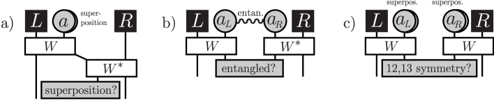
Figure 3: EPR testing procedures. a) The test from Section 3.2. b) A modified test with two ancillas. c) The Hamiltonian from Section 4 can be also easily recast as an EPR testing protocol.

We now connect our two results more directly, by providing an alternative derivation of the results in Section 4. Starting from the EPR testing protocol of Section 3.2, we turn it into a non-local Hamiltonian violating the generalized area law, using Kitaev’s circuit-to-Hamiltonian construction. In fact, we use a slight variant of the EPR testing protocol, which uses two ancillas (see Figure 3b), as it translates to a Hamiltonian more easily.

We first describe the modified EPR testing protocol. Alice has two registers, $L\otimes a_{L}$, and Bob has two registers denoted $a_{R}\otimes R$, where $R,L$ are of large dimension $D$ and $a_{R}$,$a_{L}$ are of constant dimension $d$. They wish to check whether their joint state $|\psi\rangle_{LR}$ on registers $L\otimes R$ is maximally entangled. First, Alice and Bob pre-share a maximally entangled state on $a_{L}\otimes a_{R}$:

$$|\phi_{d}\rangle=\frac{1}{\sqrt{d}}\sum_{i=1}^{d}|i\rangle_{a_{L}}|i\rangle_{a_{R}}$$ (51)

Second, Alice applies the unitary $W=\sum_{i=1}^{d}|i\rangle\langle i|\otimes U_{i}$ to $a_{L}\otimes L$, and Bob applies $W^{*}$ to $a_{R}\otimes R$. Finally, they apply a projective measurement on $a_{L}\otimes a_{R}$ of the state $|\phi_{d}\rangle$ (51). It is not difficult to see that this too is an EPR testing protocol; the test passes with probability close to 1 if and only if the original state $|\psi\rangle_{LR}$ was very close to the maximally entangled state.

To encode this protocol into a Hamiltonian via the circuit-to-Hamiltonian construction, we use two independent, two-step clocks. (We will think of the circuit $W$ as well as $W^{*}$ as applied in a single time step). The Hamiltonian will thus act on four registers, $L,R$ and two enlarged registers, $A_{L}=a_{L}\otimes C_{L}$ and $A_{R}=a_{R}\otimes C_{R}$ with $C_{L},C_{R}$ being the two $2$-dimensional spaces of the two clocks, respectively. We write the basis states of $A_{L},A_{R}$ as $|0,i\rangle$ and $|1,i\rangle$ for $i\in\{1,..,d\}$.

The Hamiltonian consists of the following terms. An “initialization” and “output” term on $A_{L}\otimes A_{R}$:

$$H_{M} =\sum_{s=0}^{1}\sum_{i,j=1}^{d}|s,i\rangle\langle s,i|_{A_{L}}\otimes|s,j\rangle\langle s,j|_{A_{R}}-\sum_{s=0}^{1}\sum_{i=1}^{d}|s,i\rangle\langle s,i|_{A_{L}}\otimes|s,i\rangle\langle s,i|_{A_{R}}$$ (52)

whose ground states have the form $|1,i\rangle|0,j\rangle$ and $|0,i\rangle|1,j\rangle$ for any $i,j$, but more importantly $\frac{1}{\sqrt{d}}\sum_{i=1}^{d}|0,i\rangle|0,i\rangle$ and $\frac{1}{\sqrt{d}}\sum_{i=1}^{d}|1,i\rangle|1,i\rangle$. These two states are maximally entangled states of the ancillas when the “clocks” are both $0$ (initialization) or both $1$ (output).

Second, we have the “left-computation-checking” Hamiltonian, which acts on the registers $a_{L}$ and $L$:

$$H_{L} =\frac{1}{2}\sum_{i=1}^{d}\left(|0i\rangle\langle 0i|+|1i\rangle\langle 1i|\right)_{a_{L}}\otimes\mathbb{I}_{L}-\frac{1}{2}\sum_{i=1}^{d}|1i\rangle\langle 0i|\otimes W-\frac{1}{2}\sum_{i=1}^{d}\otimes|0i\rangle\langle 1i|\otimes W^{\dagger}.$$ (53)

Similarly, we define $H_{R}$, the “right-computation-checking” Hamiltonian which acts on $A_{R}$ and $R$, replacing $W$ by $W^{*}$ and $W^{\dagger}$ by $W^{T}$:

$$H_{R} =\frac{1}{2}\sum_{i=1}^{d}\left(|0i\rangle\langle 0i|+|1i\rangle\langle 1i|\right)_{a_{R}}\otimes\mathbb{I}_{R}-\frac{1}{2}\sum_{i=1}^{d}|1i\rangle\langle 0i|\otimes W^{*}-\frac{1}{2}\sum_{i=1}^{d}|0i\rangle\langle 1i|\otimes W^{T}.$$ (54)

The final Hamiltonian, $H=H_{M}+H_{L}+H_{R}$ is our desired counterexample. We claim that its unique, frustration-free ground state is the “history” state

$$|\Psi\rangle =\frac{1}{\sqrt{d}}\sum_{i=1}^{d}\left(|0,i\rangle_{a_{L}}+\left(W\otimes\mathbb{I}\right)|1,i\rangle_{a_{L}}\right)\left(|0,i\rangle_{a_{R}}+\left(\mathbb{I}\otimes W^{*}\right)|1,i\rangle_{a_{R}}\right)|\phi_{D}\rangle_{LR}.$$

It is not difficult to check that this is a maximally entangled state of dimension $dD$, by observing that the Schmidt rank is $dD$ and the coefficients are uniform.

7 Discussion, related work and Open Questions

We have shown that in both the context of EPR testing, as well as ground states of Hamiltonians, constant resources suffice to enforce what seems to be a global property. Our results are reminiscent in spirit to the classical PCP theorem, or more generally to property testing. The common theme is that a small amount of resources (bits checked, Hamiltonian interactions, qubits transmitted, etc.) serve to verify the properties of some large object. However, the fact that such highly non-local properties as global entanglement can be detected using local resources seems rather counter-intuitive, and calls for further investigation in other contexts.

Our results leave many questions open. Below we discuss them as well as the broader context of these results.

The Area Law question Of course, the major open question of the 2-D area law, which was the main motivation for this work, is left wide open. A more modest goal would be to reduce the degree in our construction to a constant. Such a step already seems to require significant progress in our understanding of related notions, e.g., parallel circuit-to-Hamiltonian constructions (see e.g.,[12]), and quantum expanders which are geometrically constrained, as well as the notion of quantum degree reduction, as a possible route towards quantum PCP [1]. Alternatively, it might be true that the generalized area law does in fact hold with bounded-degree bounded-strength Hamiltonians.

Indeed, such a conjecture is not unplausible, and could potentially be motivated by the following intuition. The area law had been long believed, without proof, to be related to another very important physical property of gapped Hamiltonians: the exponential decay of correlations in the ground state. This means that a Hamiltonian has an associated correlation length $\xi$ such that $|\langle{AB}\rangle-\langle{A}\rangle\langle{B}\rangle|\leq\|A\|\,\|B\|\,e^{-\ell/\xi}$ where $\langle{X}\rangle:=\langle G|X|G\rangle$ and $A,B$ are observables separated by a distance $\ell$. Such an exponential decay is known to hold on a lattice of any constant dimension, and in fact in any constant-degree graph [25] It is perhaps natural to conjecture that if correlations in gapped Hamiltonians are in this way “local”, entanglement is also local; One way to quantify this is with the area law conjecture. However, we stress that only in 1-D this implication is known to hold [11].

Our results (in particular Theorem 7) provide a counterexample to another possible version of the area law: one in which the interaction degree is bounded, but the norms of the interactions are required to be bounded only accross the cut, and otherwise they can be polynomially large. The rationale of this condition is that large norm terms on each side of the cut should only increase the entanglement within the two regions on each side of the cut and therefore by monogamy of entanglement only decrease the entanglement across the cut. Our counterexample suggests that the above monogamy-of-entanglement argument is too naive.

Another possibile version of the area law that might still hold is that a subsystem with dimension $d_{i}$ at distance $\ell_{i}$ from the cut can contribute at most $\log(d_{i})e^{-\ell_{i}/\xi}$ entanglement, where $\xi$ is the correlation length. Attempting to strengthen our counter-example may either rule these conjectures out or, in failing to do so, give a hint of how they might be proved.

We note that the implications of an(y of the above forms of an) area law for general systems are not yet fully understood. For ground states of gapped one-dimensional systems, proving an area law was an important step towards proving that they can be efficiently described [22] and that these descriptions can be found efficiently [4, 30]. For Hamiltonians on general graphs, a partition into pieces with subvolume entanglement scaling (i.e. region $S$ has $\leq\varepsilon|S|$ entropy) would imply a classical description accurate enough to be incompatible with the quantum PCP conjecture [10]. Since entropy is a way to count effective degrees of freedom, another interpretation of area laws is that a quantum system can equivalently be represented by a theory living on its boundary. This idea is known as the holographic principle, and is currently a major conjecture in quantum field theory [35]. It remains to be clarified whether an area law of any of the suggested forms can lead to a more succinct description of the ground states.

Related work There are several related works that we would like to mention. First, Gottesman and Hastings [14], Irani [26], and Movassagh and Shor [32] have examined qudit chains with highly entangled ground states for Hamiltonians whose gaps are inverse-polynomial. To the best of our knowledge, our results cannot be derived in a straightforward manner from these works. Here, we focus on spin chains with a constant gap. One can attempt to get a constant-gap version of the above constructions by using the strengthening gadgets of Nagaj and Cao [13] as we did in this paper. However, this fails to provide the desired counterexample, since these gadgets introduce a complicated geometry of interactions, and we would need to apply them for every edge. Thus, the size of the cut in the resulting graph would no longer be small. It is crucial that in our present construction, the middle link is unchanged; only the rest of the interactions need to be strengthened by gadgets.

We mention another relevant prior work [20, 23], which described a state on a one-dimensional chain with a large amount of entanglement across cuts (say $\log n$) but only short-range correlations. The claim about decaying correlations here is rather subtle: two regions that are separated by a distance $\ell$ from each other and $\ell^{\prime}$ from the boundary have correlation no greater than $e^{-\ell/\xi}(1+ne^{-\ell^{\prime}/\xi})$. In this way it avoids contradicting the relation between decaying correlation and area law from [11]. See [23] for further discussion. This result is incomparable to ours because the states in question are not ground states of a gapped $O(1)$-local Hamiltonian.

More general implications Finally, we believe that our results point at a potentially useful link between two seemingly unrelated topics. Our paper shows that a counterexample to the generalized area law can be derived from an entanglement testing protocol of limited communication and converting it into a Hamiltonian using Kitaev’s circuit-to-Hamiltonian construction. Our area-law violating Hamiltonian can be viewed as a “tester” of its highly entangled ground state, where the norm of the Hamiltonian terms along the cut corresponds to the communication complexity of the protocol. Can any area-law-violating Hamiltonian be connected to an entanglement-testing protocol with communication pattern corresponding to the interaction graph of the Hamiltonian? More generally, in what ways can Hamiltonians be viewed as testers for their ground states? Whether such a “translation” always exists between entanglement testing protocols of limited communication, and entangled ground states of Hamiltonians with limited interactions between different parts of the system, remains to be explored. Making such an equivalence rigorous might open up a whole new set of tools to studying the area law question, and more generally, help develop better intuition for local Hamiltonians and their ground states. A related question is whether EPR testing is in fact equivalent in some sense to the property of being a quantum expander.

8 Acknowledgements

The authors thank the Simons Institute (the Quantum Hamiltonian Complexity program) where part of this work was done. DA acknowledges the support of ERC grant 030-8301 and BSF grant 037-8574. AWH was funded by NSF grant CCF-1111382 and ARO contract W911NF-12-1-0486. ZL was supported by NSF Grants CCF-0905626 and CCF-1410022 and Templeton Grants 21674 and 52536. DN thanks the Slovak Research and Development Agency grant APVV-0808-12 QIMABOS. MS is supported by the NSF Grant No. CCF-0832787, “Understanding, Coping with, and Benefiting from, Intractability” and by CISE/MPS 1246641. UV was supported by ARO Grant W911NF-12-1-0541, NSF Grant CCF-0905626, and Templeton Grants 21674 and 52536.

References

- [1] D. Aharonov, I. Arad, and T. Vidick. Guest column: The quantum PCP conjecture. SIGACT News, 44(2):47–79, June 2013, 1309.7495.
- [2] D. Aharonov, D. Gottesman, S. Irani, and J. Kempe. The power of quantum systems on a line. 2013 IEEE 54th Annual Symposium on Foundations of Computer Science, 0:373–383, 2007, 0705.4077.
- [3] A. Ambainis and A. Smith. Small pseudo-random families of matrices: Derandomizing approximate quantum encryption. In K. Jansen, S. Khanna, J. Rolim, and D. Ron, editors, APPROX-RANDOM, volume 3122 of Lecture Notes in Computer Science, pages 249–260. Springer, 2004, quant-ph/0404075.
- [4] I. Arad, A. Kitaev, Z. Landau, and U. Vazirani. An area law and sub-exponential algorithm for 1D systems. In Proceedings of the 4th Innovations in Theoretical Computer Science (ITCS), 2013, 1301.1162.
- [5] A. Barenco, B. André, D. Deutsch, A. Ekert, R. Jozsa, and C. Macchiavello. Stabilization of quantum computations by symmetrization. SIAM J. Comput., 26:1541–1557, 1997, quant-ph/9604028.
- [6] H. Barnum, C. Crepeau, D. Gottesman, A. Smith, and A. Tapp. Authentication of quantum messages. In Foundations of Computer Science, 2002. Proceedings. The 43rd Annual IEEE Symposium on, pages 449–458, 2002, quant-ph/0205128.
- [7] A. Ben-Aroya, O. Schwartz, and A. Ta-Shma. Quantum expanders and the entropy difference problem, 2007, quant-ph/0702129.
- [8] A. Ben-Aroya, O. Schwartz, and A. Ta-Shma. Quantum expanders: motivation and construction. In CCC, 2008, 0709.0911.
- [9] C. H. Bennett, D. P. DiVincenzo, J. A. Smolin, and W. K. Wootters. Mixed-state entanglement and quantum error correction. Phys. Rev. A, 52:3824–3851, 1996, quant-ph/9604024.
- [10] F. G. S. L. Brandão and A. W. Harrow. Product-state approximations to quantum ground states. In Proceedings of the 45th annual ACM Symposium on theory of computing, STOC ’13, pages 871–880, 2013, 1310.0017.
- [11] F. G. S. L. Brandão and M. Horodecki. An area law for entanglement from exponential decay of correlations. Nature Physics, 9:721–726, 2013, arXiv:1206.2947.
- [12] N. P. Breuckmann and B. M. Terhal. Space-time circuit-to-hamiltonian construction and its applications. Journal of Physics A: Mathematical and Theoretical, 47(19):195304, 2014.
- [13] Y. Cao and D. Nagaj. Perturbative gadgets without strong interactions, 2014. arXiv:1408.5881.
- [14] D. Gottesman and M. B. Hastings. Entanglement versus gap for one-dimensional spin systems. New Journal of Physics, 12(2):025002, 2010, 0901.1108.
- [15] D. Gross and J. Eisert. Quantum Margulis Expanders. Q. Inf. Comp., 8(8/9):722–733, 2008, 0710.0651.
- [16] S. Hallgren, D. Nagaj, and S. Narayanaswami. The local hamiltonian problem on a line with eight states is qma-complete. Quantum Information & Computation, 13(9-10):721–750, 2013.
- [17] A. W. Harrow. Quantum expanders from any classical Cayley graph expander. Quantum Inf. Comput., 8(8&9):715–721, 2008, 0709.1142.
- [18] A. W. Harrow and D. W. Leung. A communication-efficient nonlocal measurement with application to communication complexity and bipartite gate capacities. IEEE Trans. Inf. Theory, 57(8):5504–5508, 2011, 0803.3066.
- [19] M. B. Hastings. An area law for one-dimensional quantum systems. Journal of Statistical Mechanics: Theory and Experiment, 2007(08):P08024, 2007, 0705.2024.
- [20] M. B. Hastings. Entropy and entanglement in quantum ground states. Phys. Rev. B, 76:035114, 2007, cond-mat/0701055.
- [21] M. B. Hastings. Random unitaries give quantum expanders. Phys. Rev. A, 76:032315, 2007, 0706.0556.
- [22] M. B. Hastings. Quantum adiabatic computation with a constant gap is not useful in one dimension. Phys. Rev. Lett., 103:050502, Jul 2009, 0902.2960.
- [23] M. B. Hastings. Notes on some questions in mathematical physics and quantum information, 2014, 1404.4327.
- [24] M. B. Hastings and A. W. Harrow. Classical and quantum tensor product expanders. Q. Inf. Comp., 9(3&4):336–360, 2009, 0804.0011.
- [25] M. B. Hastings and T. Koma. Spectral gap and exponential decay of correlations. Communications in Mathematical Physics, 265(3):781–804, 2006, math-ph/0507008.
- [26] S. Irani. Ground state entanglement in one-dimensional translationally invariant quantum systems. Journal of Mathematical Physics, 51(2):–, 2010, 0901.1107.
- [27] R. Jain, J. Radhakrishnan, and P. Sen. Optimal direct sum and privacy trade-off results for quantum and classical communication complexity, 2008, 0807.1267.
- [28] C. Jordan. Essai sur la géométrie à dimensions. Bull. Soc. Math. France, 3:103–174, 1875.
- [29] A. Y. Kitaev, A. H. Shen, and M. N. Vyalyi. Classical and Quantum Computation. American Mathematical Society, Boston, MA, USA, 2002.
- [30] Z. Landau, U. Vazirani, and T. Vidick. An efficient algorithm for finding the ground state of 1d gapped local hamiltonians. In Proceedings of the 5th Conference on Innovations in Theoretical Computer Science, ITCS ’14, pages 301–302, 2014, 1307.5143.
- [31] A. Lutomirski, S. Aaronson, E. Farhi, D. Gosset, J. Kelner, A. Hassidim, and P. Shor. Making and breaking quantum money. In Innovations in Computer Science (ICS), pages 20–31, 2010, 0912.3825.
- [32] R. Movassagh and P. W. Shor. Power law violation of the area law in critical spin chains, 2014, 1408.1657.
- [33] I. Newman. Private vs. common random bits in communication complexity. Inf. Process. Lett., 39(2):67–71, 1991.
- [34] Y. Shi and Y. Zhu. Tensor norms and the classical communication complexity of nonlocal quantum measurement. SIAM J. Comput., 38(3):753–766, 2008, quant-ph/0511071.
- [35] B. Swingle. Entanglement renormalization and holography. Phys.Rev. D, 86:065007, 2012, 0905.1317.