Generation of entangled matter qubits in two opposing parabolic mirrors
Abstract
We propose a scheme for the remote preparation of entangled matter qubits in free space. For this purpose, a setup of two opposing parabolic mirrors is considered, each one with a single ion trapped at its focus. To get the required entanglement in this extreme multimode scenario, we take advantage of the spontaneous decay, which is usually considered as an apparent nuisance. Using semiclassical methods, we derive an efficient photon-path representation to deal with this problem. We also present a thorough examination of the experimental feasibility of the scheme. The vulnerabilities arising in realistic implementations reduce the success probability, but leave the fidelity of the generated state unaltered. Our proposal thus allows for the generation of high-fidelity entangled matter qubits with high rate.
pacs:
42.50.Pq 03.67.Bg 42.50.Ct 42.50.ExI Introduction
The distribution of entanglement between macroscopically separated parties constitutes a key ingredient of quantum information networks Nielsen and Chuang (2000); Kimble (2008). A quantum network is composed of nodes, for processing and storing quantum states, and channels linking the nodes. The implementation of quantum nodes is a major challenge: different approaches are currently being pursued, most of them involving single emitters, such as ions, atoms or nitrogen-vacancy centers Olmschenk et al. (2009a); Hofmann et al. (2012); Ritter et al. (2012); Bernien et al. (2013), even though they are inherently probabilistic.
Photonic channels are especially advantageous, as optical photons can carry information over long distances with almost negligible decoherence. In practice, there are two types of these channels: optical fibers and free space. Optical fibers are capable of transmitting single photons over large distances with high efficiency while suffering from effects like birefringence or dispersion. The free space channel, however, does not suffer from these effects, but photon losses due to beam wandering or beam broadening, for example, can play a prominent role. Thus both types of photonic channels have their own pros and cons Gisin et al. (2002) and distribution of entangled photonic qubits was successfully demonstrated for both of them, over a distance of 200 km Dynes et al. (2009) using optical fibers and over 144 km Ursin et al. (2007) in free space.
The main issue with a free-space channel is the low photon-collection efficiency. This can be improved by placing the single emitter at the focus of a parabolic mirror Maiwald et al. (2012), which in addition enhances the atom-field interaction Leuchs and Sondermann (2013); Fischer et al. (2014).
Here, we propose to use two opposing parabolic mirrors to prepare maximally entangled states of two matter qubits at the corresponding focal points. Our scheme involves an extreme multimode scenario ,i.e., the atoms couple to a continuum of modes of the radiations field, due to the fact that the parabolic mirror is a half-open cavity. Thereby, we deal with intrinsic multimode effects like spontaneous decay processes, which are usually considered as sources of undesirable decoherence. Interestingly enough, we will be able to use these effects as tools for entanglement generation, rather than avoiding them.
In other multimode schemes Moehring et al. (2007) each deviation from the ideal situation, such as non perfect mode matching, leads to a reduction of the fidelity of the generated state. In contradistinction, our scheme is robust against the vulnerabilities that arise in experimental implementations: they reduce the success probability, but leave the fidelity unaltered (and, accordingly, it can be very high). As outlined below, this is due to the use of photons originating from circular-dipole transitions, a suitable choice of the quantization axis and direct dispersive probing of the qubit states.
This paper is organized as follows. In Sec. II we advance the basic ingredients of our scheme, which is fully analyzed in Sec. III by resorting to a photon-path representation Alber et al. (2013); Milonni and Knight (1974) especially germane for a multimode description. To incorporate the boundary conditions for the relevant solution of the Helmholtz equation, we apply a semiclassical approximation Berry and Mount (1972); Maslov and Fedoriuk (1981). We discuss the results in Sec. IV and their feasibility in Sec. V. Finally, our conclusions are briefly summarized in Sec. VI.
II Remote entanglement preparation
Our setup, as roughly schematized in Fig. 1, consists of two parabolic mirrors opposing each other, so they direct any electromagnetic field from one focal point to the other with great efficiency.
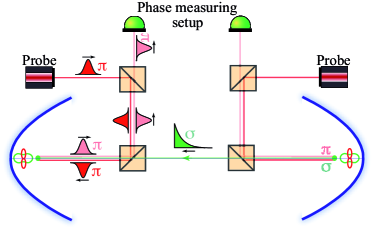
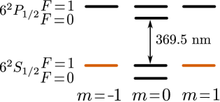
We consider a trapped ion at the focus of each parabolic cavity. This ion has quite a suitable hyperfine electronic structure due to its nuclear spin . We concentrate on the level scheme formed by the levels and shown in Fig. 2. The logical qubit is defined by the levels and (note the different choice in Ref. Olmschenk et al. (2007, 2009a)). The corresponding dipole matrix elements are denoted by , where and are the wave functions of the different states.
The basic idea is to initially prepare ions 1 and 2 in the states
| (1) | |||
and use the time evolution to generate an entangled state. For that, we notice that ion 1 can decay into three different states: , emitting a right-circularly polarized () photon, , emitting a left-circularly polarized () photon, and , emitting a linearly polarized () photon. Because we do not know which of the three mentioned processes actually take place, the complete state of the system is a linear superposition of the three corresponding probability amplitudes. As a consequence, ion 1 and the radiation field get entangled.
The geometry of the setup ensures that the photon wave packet generated by the spontaneous decay of ion 1 propagates to the focus of the second parabola, where it may excite ion 2. After the absorption, the second ion is in the state , if it absorbs a polarized photon, and in the state , if it absorbs a polarized photon. These absorption processes map the field state onto the state of the second ion and thereby generating entangled matter states.
The ion 2 being in an excited state (in the manifold), is affected by spontaneous decay. So, we have to perform a state transfer from the manifold to the manifold that is radiatively stable. One might think in using a single -pulse, but this is not a proper solution because the photon wave packet radiated by ion 1 has a certain temporal width, which yields a probabilistic determination for the time when the photon is absorbed by ion 2. If ion 2 is still in the ground state when we apply the -pulse, the pulse does not have the desired effect. If we wait a certain time to make sure that the absorption has already taken place before applying the -pulse, it is also likely that the spontaneous decay process back to the manifold may have already occurred. We remind that unit excitation probability can only be achieved with a time-reversed single-photon wave packet Stobińska et al. (2009).
We suggest to use instead the spontaneous decay itself. To that end, we have to take into account the different decay channels. For example, consider that ion is in the state : it can decay into the states , and . But only the last process generates entanglement. In a similar way, one can treat the case that ion is in the state .
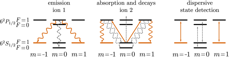
To discard the undesired decay processes, we have to perform a postselection. Since only in case of successful entanglement generation both ions end up in the qubit state, by probing the occupation of the qubit states we discard the undesired decay processes. This can be performed with negligible loss of entanglement by using dispersive state detection. It suffices to couple weak off-resonant coherent pulses to the transitions from to : population is then detected by the phase shifts imprinted onto the coherent states. This procedure allows us to check the population of the qubit states while preserving the possible linear superpositions and thus does not disturb the entangled state.
Furthermore, this postselection also detects photon losses, so that the scheme is loss tolerant. This is due to the fact that upon photon loss ion 2 remains in and post selection is probed on -transitions, which are for either forbidden or detuned so strongly that no phase shift of the probe pulse occurs. Of course, losses reduce the success probability, but the fidelity after a successful postselection is not affected. The low success probability can be overcome with a high repetition rate.
All the steps for generating entangled states described above are depicted in Fig. 3.
III Theoretical analysis
III.1 System Hamiltonian
In the rotating-wave and dipole approximations, the Hamiltonian of the foregoing system can be written as
| (2) |
where
| (3) | |||||
Here, describes the dynamics of the matter. We indicate by (excited) the set of states in the manifold and by (ground) the set of states in the manifold . The vectors , represent states of the ion 1 and ion 2 living in , with energies and , respectively. gives the dynamics of the field, characterized by the annihilation () and creation () operators of the modes (of frequency ) that couple to the ions (they depend on the boundary conditions). Finally, the interaction between the ions and the field is given by , wherein H.c. stands for the Hermitian conjugate and
and being the position of the first and second ion, respectively. The orthonormal mode functions are solutions of the Helmholtz equation with the proper boundary conditions, fulfilling, in addition, the transversality condition .
III.2 Photon-path-representation
Since only one excitation is available in our initial state, and the Hamiltonian (III.1) preserves the number of excitations, the state of the system at time can be written as
| (5) | |||||
where is the vacuum state and a single-photon state of the radiation field. The amplitude describes the evolution when the field is in the vacuum, the first ion is in one of the excited levels and the second ion is in one of the ground levels and an analogous interpretation for . The amplitude is related to the evolution when there is an excitation in the field mode and both ions are in one of the ground electronic levels .
Now, we can solve the time-dependent Schrödinger equation, with the ansatz (5). If we assume that the field is initially in a vacuum state and we use the Laplace transform, we get, after eliminating the transforms of the probability amplitudes for photonic excitations ,
| (6) |
where indexes the ions, and
| (7) |
The function
| (8) |
with
| (9) |
describes all possible photon emission and absorption processes and encodes the whole geometry of the setup through the modes . Its explicit calculation turns to be a difficult task, although in Appendix A we sketch a semiclassical method.
Equation (6) can be recast in a suggestive vectorial form
| (10) |
where the functions are arranged in a vector and is a diagonal matrix which represents the term . The contribution can be split as
| (11) |
where is equal to , with being the spontaneous decay rate in free space, and embodies exponentially decaying terms of the form . In principle, one could try to perform an inverse Laplace transform to solve (10). However, this involves finding the poles of the integrand, which is a formidable task because depends itself on in a highly nontrivial way.
To determine we use instead an alternative route based on the Neumann expansion
| (12) |
If we take we get
| (13) |
and each term in the series can be immediately Laplace inverted. The price we pay is that we have to deal with an infinite series.
In most circumstances, only a few terms contribute to Eq. (13): since each summand is damped by an exponential of the form , and when applying the inverse Laplace transform, each term leads to a Heaviside step function, i.e., a retardation, shifted into the positive direction by time . If we are looking at the evolution in a finite time interval, we can neglect terms which are so far retarded that they do not contribute.
The time interval of interest in our setup is of the order of , which is the typical travel time of a photon to go from the first to the second ion and being the focal length of the mirrors and the separation between foci. In consequence, we can neglect all terms in the sum; as shown in Ref. Alber et al. (2013), the higher-order terms are relevant when the focal length is comparable with the wavelength, which is not the case for our actual mirrors Maiwald et al. (2012) (2.1 mm and wavelength nm).
IV Results
If one uses the method of the preceding section in the time interval , it turns out that only four of the atomic probability amplitudes () are of relevance:
| (14) |
If the hyperfine splitting is large in comparison to the spontaneous decay rate , as it happens for in the time window of interest, we can also neglect .

In Fig. 4 we plot the excitation probabilities of the two ions for vanishing Zeeman splitting. As discussed in Sec. II, the process generates an entangled state if one uses the states and of the second ion as qubit. But these states do not form a stable qubit; spontaneous decay transfers them to the ground states and by emitting a single photon. By detecting whether or not both ions are in one of the states , we check if the entanglement generation was successful.
The postselection is equivalent to a von Neumann measurement described by the projection operator
| (15) |
where () correspond to the states of the logical qubit. In addition, we also have to deal with the photon emitted in the transfer from the excited to the ground states. This photon, which carries information about the state of the ions, might cause decoherence and therefore destroy the entangled state generated by the time evolution. To certify that this is not the case, we have to trace out the uncontrolled photonic degrees of freedom, which amounts to know
| (16) |
This density matrix is evaluated in Appendix C. In the limit with , we have that
| (17) |
The parameter characterizes the Zeeman splitting of the energy levels: is the splitting in the manifold and the splitting in the manifold. Note that the magnetic field has the same orientation and strength for both ions.
For , which is justified in our experimental setup Maiwald et al. (2012), we get
| (18) |
which corresponds to a maximal entangled state with a success probability . Of course, in a real experiment, one has to take additional effects into account. As we explore in the next Section, it should be possible to achieve free-space communication over several kilometers.
V Experimental feasibility
V.1 Realistic parabolic mirrors
In a real setup, the parabolic mirror does not cover the full solid angle. Actually, in our parabolic mirror Maiwald et al. (2012) we have
| (19) |
whereby the angle gives the front opening of the parabola and the angle accounts for the hole on the backside for inserting the ion trap. This has to be taken into account in integrations as in Eq. (A).
Furthermore, our mirrors are made out of aluminum, which has a finite electrical conductivity. The properties of the material are well described by introducing a frequency dependent dielectric constant . In our case Rakić et al. (1998). Now, we have to split the field in a transverse electric (TE) and a magnetic (TM) part and apply Fresnel equations to deal with the boundary conditions. But these equations are different for the two basic polarizations and give angle-dependent phase shifts and reflectivities, which leads to a further reduction of the efficiency for entanglement generation. One might think that this effect could also reduce the fidelity of the entangled state but this is not the case. Such a reduction could occur if a () decay of the first ion could drive a ( transition of the second ion, but due to the symmetry this does not occur.
This is obvious from the following reasoning: After collimation by the parabolic mirror, the polarization vector of the electric field in the exit pupil of the parabolic mirror reads Sondermann et al. (2008)
| (20) | ||||
with the distance to the optical axis in units of the mirror’s focal length, the azimuthal angle, and and the unit vectors in radial and azimuthal direction, respectively. Upon reflection on the parabolic surface, these vectors correspond to TM- and TE-components. The influence of the metallic mirror can be accounted for by additional complex pre-factors which depend on only. It is straightforward to show that the overlap of this modified field with the state of opposite helicity vanishes.
We can sum all the above effects in a factor which has to be multiplied with the probability for a successful entanglement creation to take the more realistic mirrors into account: corresponds to perfectly conducting parabolic mirrors that cover the full solid angle. In the specific case treated here, we have .
V.2 Free-space versus fiber-based transmission
Our scheme is designed to be compatible with free-space communication by photonic qubits, for it does not rely on the strong coupling regime, but on intrinsic multimode effects like spontaneous emission.
There are other multimode schemes, such as the one in Ref. Moehring et al. (2007), which might be adapted to free-space communication, but our proposal offers considerable advantages. The scheme in Ref. Moehring et al. (2007) heavily relies on fibers as mode filters to achieve almost perfect mode matching on a beam splitter and, besides, the fidelity is mainly limited by the fact that the postselection is performed on the radiation field and is sensitive to dark counts of the detectors. In contrast, in our proposal, postselection is performed on the ions, which circumvents detector dark counts.
Of course, we have to take into account experimental imperfections, mainly connected with the free-space transmission of the one-photon wave packet. This gives rise to beam wandering and phase-front distortions due to atmospheric turbulences Ursin et al. (2007). In both cases, the intensity at the focus is reduced Lieb (2001); Leuchs et al. (2008); April et al. (2011), affecting the success probability. Once the distance between the two parabolic mirrors becomes large enough, beam broadening plays a crucial role, which also results in a lower success probability. All these effects, however, diminish the success probability but seem to leave the fidelity rather untouched, which is of big importance for practical applications.
One could also think about the transmission of the photon from ion 1 to ion 2 via an optical fiber. This would circumvent all problems related to atmospheric transmission, but, due to their complex polarization pattern, cf. Eq. (20), the photons collimated by the parabolic mirror have subunit overlap with a fundamental Gaussian mode with circular polarization. Hence the efficiency in coupling these photons to a single-mode fiber is limited to a maximum of 49 % Sondermann et al. (2008). Therefore, fiber transmission alone would limit the success probability of our entanglement scheme to 24 %. Moreover, the strong attenuation of ultraviolet radiation in standard optical fibers reduces the success probability by orders of magnitude, even for distances about 1 km. Finally, fibers are not well suited to perform communication via polarization coding Gisin et al. (2002), as in our scheme.
V.3 Postselection
As advanced in Sec. II, the best way to perform postselection seems to probe qubit states directly by dispersive state detection. This can be implemented by coupling weak coherent-state pulses to the transitions from to . Population in the states is then detected by the phase shifts imprinted onto the coherent states. The detuning and pulse amplitudes can be chosen such that one is far from saturating the respective transitions. For example, choosing an on-resonance saturation parameter of and a detuning of two linewidths, the excitation probability is about , while the phase of the coherent pulse is shifted by , according to the formalism of Ref. Sondermann and Leuchs (2013).
One has to balance the amplitude and the detuning of the incident coherent state carefully. Larger amplitudes and smaller detunings result in lower error probabilities for detecting the phase of the coherent state, but also enforce a stronger excitation of the ion. The latter might lead to transferring the ion out of the state during state detection, hindering the phase shift of the coherent state and hence resulting in erroneous postselection. Furthermore, the reflectivity of the beam splitters in front of the parabolic mirrors not only affects the success probability of our entangling scheme, but also influences the error in measuring the phase of the coherent state.
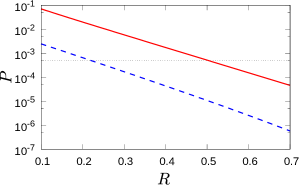
We compute the corresponding error probabilities according to the Helstrom bound Bergou (2010). The a priori probabilities in this calculation are obtained from all relevant branching ratios, excitation probabilities, and reflectivities. The amplitude of the coherent state is chosen such that the probability to excite the ions with the probe pulse is . We also choose this value as an upper bound for the acceptable error probability. This is motivated by the fact that postselection schemes probing the states are limited in fidelity to values by the branching ratio of the state to the state of 0.5%. Keeping all errors in our postselection scheme an order of magnitude below this value is reasonable and desirable.
The minimum error probabilities as a function of the reflectivity of the beam splitters coupling the coherent states into the parabolic mirrors is plotted in Fig. 5. First, we determined the reflectivity for the beam splitter in front of ion 1 that ensures being below the error threshold for a set of suitable parameters, yielding . Next, this result was used in the calculations for ion 2, leading to . From these reflectivity values one would obtain a reduction of the success probability for entanglement generation by 61 %.
In practice the Helstrom bound will not be reached entirely, with the actually obtainable error probability depending on the method employed for measuring the phase of the probe pulse. Nevertheless the error threshold marked in Fig. 5 can be reached. This may be achieved at the cost of using beam splitters with larger reflectivities and thus accepting lower success probabilities.
To guarantee that the entangled state is not destroyed, we have to ensure that no information about the state of the qubit is extracted by our postselection. The latter condition is fulfilled if the magnetic field fixing the quantization axis is sufficiently small (,i.e., the frequency shifts caused by the Zeeman effect are small compared to the spontaneous decay rate), so that the phase shift imprinted by an ion in the Zeeman state will be practically the same as for the other ion in the state. Therefore, probing the qubit dispersively will not project the ions into one of these states and entanglement is preserved. The parameter set in Fig. 5 yields a fidelity of 0.998 when postselecting. Even higher fidelities can be reached by larger beam splitter reflectivities (accompanied by decreasing success probabilities), lower pulse amplitudes or longer pulse lengths. A lower pulse amplitude has to be compensated for by larger beam splitter reflectivities or longer pulse lengths. The latter in turn affects the repetition rate.
V.4 Repetition rate
We finally estimate the achievable repetition rate. Typically, an experimental cycle starts with Doppler cooling the ion, which takes about 200 s for the ions treated here Olmschenk et al. (2009b). For the trap frequencies inherent to the parabolic mirror trap, 500 kHz in radial direction and 1 MHz along the optical axis, the average number of motional quanta according to the Doppler limit is 20 and 10, respectively. This corresponds to widths of the ion wave function in position space about 0.13 and 0.07 wavelengths. With these numbers we estimate that the ions experience 78 % of the focal intensity obtained by diffraction limited focusing. Applying only Doppler cooling the success probability of our entanglement scheme would be reduced accordingly. One could additionally apply resolved side-band cooling, but the increase of the success rate is obviously accompanied by a lower repetition rate due to the elongated cooling procedure. Furthermore, as soon as there is a broadened focus due to incompletely compensated atmospheric aberrations etc. the above spread of the ion’s wave function is negligible.
After cooling, both ions have to be prepared in the state which takes less than 1 s Olmschenk et al. (2007). Additionally, ion 2 has to be flipped to the state . This can be accomplished in 6 s using microwaves Olmschenk et al. (2007) or in 100 ps applying Raman transitions Campbell et al. (2010). Likewise, ion 1 is brought to the state by an optical -pulse on a time scale smaller than a nanosecond. The postselection requires around 80 s, as it was outlined in Sec. V.3. The photon traveling time from ion 1 to ion 2 is of the order of 10 s for distances of a few kilometers. At least, the same time has to be spent in communicating the postselection via a classical communication channel. Thus, the time spent for state preparation, attempting entanglement of the ions and postselection is on the order of 100 s.
From the numbers given above, one would estimate a repetition rate of 3.3 kHz if Doppler cooling is applied after each entanglement attempt. One could increase the repetition rate if Doppler cooling is performed regularly after a certain number of entanglement trials. Since one entanglement trial takes about 100 s, a repetition rate in excess of 10 kHz is not feasible, unless one accepts a reduced fidelity and/or success probability. Assuming a realistic heating rate of 10 quanta per ms McLoughlin et al. (2011), the spread of the ion wave function would roughly double in radial direction within 8 ms. Accepting the accompanying, continuously increasing loss of success probability, one could enhance the repetition rate towards 9.8 kHz, which is close to the inverse of the duration of one entanglement trial. Anyhow, in every experimental realization, the repetition rate is dictated by the specific requirements on fidelity, success probability and inter-ion distance.
VI Concluding remarks
In summary, we have presented a scheme for preparing maximally entangled states of two matter qubits with high fidelity by using a free-space channel. The qubits are encoded in the level structure of two distant ions located at the foci of two parabolic mirrors. The theoretical description of the setup involves an extreme multimode scenario to model the radiation field and a level structure far more complicated than a simple two level atom.
We have used a semiclassical photon-path representation to deal with the boundary conditions at the two parabolic mirrors, which leads to a intuitive representation of the quantum dynamics of the two ions and the radiation field.
To obtain a more realistic description, we have focused on the experimental details in Ref. Maiwald et al. (2012) and on more realistic boundary conditions. Our results confirm the feasibility of the scheme to achieve reasonable success probabilities, which in combination with a relatively high repetition rate leads to a proper rate for preparing entangled matter qubits. Indeed, we expect an entanglement rate of 54 per second under diffraction-limited focusing.
One of the main issues is the fidelity of these states. Our scheme is robust against imperfections arising in the experimental implementation. All these effects reduce the success probability of entanglement generation, but leave the fidelity untouched.
We hope that our work is a step towards an experimental realization of remote entangled matter qubits in free space, which is a key building block for future quantum technologies.
Acknowledgements.
N. T., J. Z. B., and G. A. acknowledge support by the BMBF Project Q.com and CASED III. M. S. and G. L. are grateful for the financial support of the European Research Council under the Advanced Grant PACART. Finally, L. L. S. S. acknowledges the support from the Spanish MINECO (Grant No. FIS2011-26786).Appendix A Determination of the functions
We describe here how to evaluate the functions . The main idea is to relate these functions with the Laplace transform of the retarded Green’s functions of the vectorial d’Alembert operator, which can be determined by using the multidimensional JWKB approximation. This is valid when the typical wavelength is much smaller compared to the focal length of the cavities . Besides, this will enable us to clarify the retardation effects in due to the propagation of a photon wave packet.
Let us introduce the functions
| (21) |
where denotes the Laplace transform and is the Green’s function of the vectorial d’Alembert operator satisfying the appropriate boundary conditions. We recall that can be expanded in terms of the mode functions as
| (22) |
where is the dyadic product and the Heaviside step function. We can immediately show that
| (23) | |||||
If we compare with our definition of , viz
| (24) |
we see that the two expressions just differ by
| (25) |
This term can be neglected by using the same argument employed to justify the rotating-wave approximation and, therefore, to a good approximation, we can identify with .
Our next step is to get a manageable expression for these functions. To achieve this we divide our cavity in three regions:
-
1.
A sphere of radius centered around the first ion. has to be chosen such that , but small when compared with and .
-
2.
The whole volume, except the spheres centered around the ions.
-
3.
A sphere of radius centered around the second ion.
In regions 1 and 3, we use the free-space propagator, while in region 2 we use a JWKB approximation for the Green’s function (which is presented in Appendix B). After matching the resulting expressions, we obtain
where
denotes the solid angle around the ions covered by the parabolic mirrors and denotes the transition frequency of the corresponding optical transitions.
Appendix B The multidimensional JWKB method
As heralded in appendix A, we derive here semiclassical approximations for the functions by using multidimensional JWKB method Maslov and Fedoriuk (1981). In region 1, we use the free-space Green’s function
| (28) |
and, since , we can use the approximation
| (29) | |||||
If we introduce for each focus a system of spherical coordinates, with the focus lying at the origin, we can represent this Green’s function in region 1 as
| (30) |
where has been defined in Eq. (A).
We use the multidimensional JWKB method to propagate this expression to the second focus; that is, in region 2. Therefore, we construct the rays from geometrical optics. The result reads
| (31) | |||||
We have introduced the typical time and we have neglected contributions that are small when . Of course, in Eq. (31) we have taken into account that the parabola covers only a finite solid angle .
Next, we have to take care of region 3. Here, we use the free-space propagator, because the JWKB method would cause a singularity at the second focus. The mentioned propagator for the electric field, which can be derived by using , is given by
| (32) | |||||
where . If we apply this expression to our problem with the dyadic Green’s function we finally obtain
| (33) |
In the limiting case that the mirrors cover the full solid angle, we obtain .
So far, we have neglected the fact that we could also continue the described geometrical rays, which would add further terms to our expression for the dyadic Green’s function. But as long we are only interested in time intervals we can neglected this continuation of the rays. Of course, the relation
| (34) |
holds true.
We have to calculate also and . We are retaining only the dominant contribution, which is associated to the free-space part of the Green’s function. The problem is that this part leads to a divergent expression that needs to be regularized. For simplicity, we only take care of the problem , because the symmetry of the problem leads to the general solution. So, we get
| (35) |
In this expression terms of the form appear. By applying a formal Taylor expansion, we get
As one can see the sum in the second line contains singular terms, which lead to the divergent Lamb-shift appearing after the dipole approximation. If we neglect those terms, we get
| (37) |
which, given the symmetry of the problem, gives the general solution
| (38) |
From here, we immediately get
| (39) |
for . Since the time evolution of the different probability amplitudes is dominated by rapid oscillations of the form , one can replace each by and we thus get directly the result in Eq. (A).
Appendix C Tracing out the photonic degrees of freedom
To calculate the fidelity of the entangled state generated by our scheme, we have to trace out the uncontrolled photonic degrees of freedom, which in general cause decoherence and destroy entanglement. Our goal is to determine the reduced density matrix
| (40) | |||||
The second line of this equation, which denote is of main interest, because the ions are affected by spontaneous emission and both of them will be in the ground state after a short while. To obtain an expression for we have to evaluate an infinite sum. It is possible to rewrite this sum to a finite sum by using the functions . The result is the following expression
| (41) |
References
- Nielsen and Chuang (2000) M. Nielsen and I. L. Chuang, Quantum Computation and Quantum Information (Cambridge University Press, Cambridge, 2000).
- Kimble (2008) H. J. Kimble, Nature 453, 1023 (2008).
- Olmschenk et al. (2009a) S. Olmschenk, D. Matsukevich, P. Maunz, D. Hayes, L. M. Duan, and C. Monroe, Science 323, 486 (2009a).
- Hofmann et al. (2012) J. Hofmann, M. Krug, N. Ortegel, L. Gérard, M. Weber, W. Rosenfeld, and H. Weinfurter, Science 337, 72 (2012).
- Ritter et al. (2012) S. Ritter, C. Nolleke, C. Hahn, A. Reiserer, A. Neuzner, M. Uphoff, M. Mucke, E. Figueroa, J. Bochmann, and G. Rempe, Nature 484, 195 (2012).
- Bernien et al. (2013) H. Bernien, B. Hensen, W. Pfaff, G. Koolstra, M. Blok, L. Robledo, T. Taminiau, M. Markham, D. Twitchen, L. Childress, and R. Hanson, Nature 497, 86 (2013).
- Gisin et al. (2002) N. Gisin, G. Ribordy, W. Tittel, and H. Zbinden, Rev. Mod. Phys. 74, 145 (2002).
- Dynes et al. (2009) J. F. Dynes, H. Takesue, Z. L. Yuan, A. W. Sharpe, K. Harada, T. Honjo, H. Kamada, O. Tadanaga, Y. Nishida, M. Asobe, and A. J. Shields, Opt. Express 17, 11440 (2009).
- Ursin et al. (2007) R. Ursin, F. Tiefenbacher, T. Schmitt-Manderbach, H. Weier, T. Scheidl, M. Lindenthal, B. Blauensteiner, T. Jennewein, J. Perdigues, P. Trojek, B. Ömer, M. Fürst, M. Meyenburg, J. Rarity, Z. Sodnik, C. Barbieri, H. Weinfurter, and A. Zeilinger, Nature Physics 3, 481 (2007).
- Maiwald et al. (2012) R. Maiwald, A. Golla, M. Fischer, M. Bader, S. Heugel, B. Chalopin, M. Sondermann, and G. Leuchs, Phys. Rev. A 86, 043431 (2012).
- Leuchs and Sondermann (2013) G. Leuchs and M. Sondermann, J. Mod. Optics 60, 36 (2013).
- Fischer et al. (2014) M. Fischer, M. Bader, R. Maiwald, A. Golla, M. Sondermann, and G. Leuchs, Appl. Phys. B 117, 797 (2014).
- Moehring et al. (2007) D. Moehring, P. Maunz, S. Olmschenk, K. Younge, D. Matsukevich, L. M. Duan, and C. Monroe, Nature 449, 68 (2007).
- Alber et al. (2013) G. Alber, J. Z. Bernád, M. Stobińska, L. L. Sánchez-Soto, and G. Leuchs, Phys. Rev. A 88, 023825 (2013).
- Milonni and Knight (1974) P. W. Milonni and P. L. Knight, Phys. Rev. A 10, 1096 (1974).
- Berry and Mount (1972) M. Berry and K. Mount, Rep. Prog. Phys. 35, 315 (1972).
- Maslov and Fedoriuk (1981) V. Maslov and M. Fedoriuk, Semi-Classical Approximation in Quantum Mechanics (Reidel, Dordrecht, 1981).
- Olmschenk et al. (2007) S. Olmschenk, K. C. Younge, D. L. Moehring, D. N. Matsukevich, P. Maunz, and C. Monroe, Phys. Rev. A 76, 052314 (2007).
- Stobińska et al. (2009) M. Stobińska, G. Alber, and G. Leuchs, Europhys. Lett. 86, 14007 (2009).
- Rakić et al. (1998) A. Rakić, A. Djurišić, J. Elazar, and M. Majewski, Appl. Opt. 37, 5271 (1998).
- Sondermann et al. (2008) M. Sondermann, N. Lindlein, and G. Leuchs, arXiv:0811.2098 (2008).
- Lieb (2001) M. Lieb, Opt. Express 8, 458 (2001).
- Leuchs et al. (2008) G. Leuchs, K. Mantel, A. Berger, H. Konermann, M. Sondermann, U. Peschel, N. Lindlein, and J. Schwider, Appl. Opt. 47, 5570 (2008).
- April et al. (2011) A. April, B. Pierrick, and P. Michel, Opt. Express 19, 9201 (2011).
- Sondermann and Leuchs (2013) M. Sondermann and G. Leuchs, J. Europ. Opt. Soc. Rap. Public. 8, 13502 (2013).
- Bergou (2010) J. Bergou, J. Mod. Optics 57, 160 (2010).
- Olmschenk et al. (2009b) S. Olmschenk, D. Hayes, D. N. Matsukevich, P. Maunz, D. L. Moehring, K. C. Younge, and C. Monroe, Phys. Rev. A 80, 022502 (2009b).
- Campbell et al. (2010) W. C. Campbell, J. Mizrahi, Q. Quraishi, C. Senko, D. Hayes, D. Hucul, D. N. Matsukevich, P. Maunz, and C. Monroe, Phys. Rev. Lett. 105, 090502 (2010).
- McLoughlin et al. (2011) J. J. McLoughlin, A. H. Nizamani, J. D. Siverns, R. C. Sterling, M. D. Hughes, B. Lekitsch, B. Stein, S. Weidt, and W. K. Hensinger, Phys. Rev. A 83, 013406 (2011).