Entanglement negativity after a global quantum quench

Abstract

We study the time evolution of the logarithmic negativity after a global quantum quench. In a 1+1 dimensional conformal invariant field theory, we consider the negativity between two intervals which can be either adjacent or disjoint. We show that the negativity follows the quasi-particle interpretation for the spreading of entanglement. We check and generalise our findings with a systematic analysis of the negativity after a quantum quench in the harmonic chain, highlighting two peculiar lattice effects: the late birth and the sudden death of entanglement.

1 Introduction

The non-equilibrium dynamics of isolated quantum systems is one of the most active research area of the last years. In a global quantum quench, a system is initially prepared in the ground state of a translationally invariant Hamiltonian $H_{0}$ and it is then left evolving with another translationally invariant Hamiltonian $H$ differing from $H_{0}$ for an experimentally tuneable parameter. Key questions in quench dynamics are whether the system reaches for long time a stationary state, how to characterise it from first principles, and how this steady state is approached in time (see e.g. Refs. [1, 2] for reviews).

Nowadays a number of advanced analytical and numerical techniques have been developed to study the quench dynamics for a variety of different situations and realistic models [3, 4, 5, 6, 7, 8]. However, many insights on these non-equilibrium dynamics came from the study of oversimplified theories such as 1+1 dimensional conformal field theory (CFT). Indeed, phenomena like the light-cone spreading of correlations [3, 9], the linear increase of entanglement entropy [10] and the structure of revivals in finite systems [11] have been first discovered in CFT, later generalised to more realistic models and even verified in experiments (see [12] for the experimental measure of the light-cone spreading of correlations).

The main goal of this paper is to shed some light on the time evolution of the entanglement between two different regions in an extended system following a quantum quench. We will quantify this entanglement by means of logarithmic negativity for which a general quantum field theory approach has been recently developed [13, 14, 15]. We consider this problem in the framework of CFT, closely following the approach introduced in Refs. [10, 9] for the time evolution of entanglement entropy and correlations. In order to understand the generality and the limits of this approach, we parallel the analytic CFT calculations with some exact numerical computations for the harmonic chain. The non-equilibrium evolution of the negativity in CFT, but for different quench protocols, has also been considered in Refs.  [16, 17].

1.1 Quench protocol

The system is prepared in the ground state $|\psi_{0}\rangle$ of the Hamiltonian $H_{0}$. The quantum quench consists in a sudden (instantaneous) change of a parameter in the Hamiltonian $H_{0}\rightarrow H$ at a given time that we set as $t=0$. Thus, the unitary evolution of $|\psi_{0}\rangle$ is

$$|\psi(t)\rangle=e^{-\textrm{i}Ht}\,|\psi_{0}\rangle\,.$$ (1)

The density matrix associated to this pure state is $\rho(t)=|\psi(t)\rangle\langle\psi(t)|$. In 1+1-dimensional CFT, the calculations become manageable when $|\psi_{0}\rangle$ is a boundary conformal state as we will explain in what follows. In this approach, analytical results have been obtained for the entanglement entropy of a single and more intervals [10], for correlation functions of primary operators [3, 9], and a few other quantities [18, 19, 20, 21]. We will not be interested here in the time evolution of the entanglement after a local quench, a subject which has been considered instead in Refs. [22, 23, 24, 25, 26, 27], but only for the entanglement entropies.

1.2 Quantities of interest

As we anticipated, we are interested here in the entanglement between two different regions, which in the case of a one dimensional system are two intervals, either adjacent or disjoint, as shown in Fig. 1. In order to define the entanglement, we should first introduce the reduced density matrix of the part $A$ of the system as $\rho_{A}={\rm Tr}_{B}\rho(t)$, where we traced over the degrees of freedom in $B$, which is the complement of $A$.

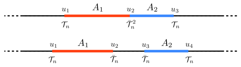
Figure 1: Configurations of two intervals in the infinite line that we consider: adjacent intervals (top) and disjoint intervals (bottom).

The entanglement of a bipartite system can be quantified by the entanglement entropy [28]

$$S_{A}=-{\rm Tr}\,\rho_{A}\ln\rho_{A}\,,$$ (2)

or alternatively by the Rényi entanglement entropies

$$S_{A}^{(n)}=\frac{1}{1-n}\ln{\rm Tr}\rho_{A}^{n}\,.$$ (3)

The limit $n\to 1$ of $S_{A}^{(n)}$ gives $S_{A}$, but $S_{A}^{(n)}$ contain much more information, since one can extract the full spectrum of $\rho_{A}$ from them [29]. Notice that, when $A=A_{1}\cup A_{2}$ is composed of two disjoint regions $A_{1}$ and $A_{2}$, the entanglement entropy quantifies only the entanglement between $A$ and the remainder of the system $B$, but not the entanglement between $A_{1}$ and $A_{2}$. In this case one can introduce the mutual information

$$I_{A_{1},A_{2}}\equiv\,S_{A_{1}}+S_{A_{2}}-S_{A_{1}\cup A_{2}}\,,$$ (4)

and, analogously, the Rényi mutual information

$$I^{(n)}_{A_{1},A_{2}}\equiv\,\frac{1}{n-1}\ln\left(\frac{{\rm Tr}\rho_{A}^{n}}{{\rm Tr}\rho_{A_{1}}^{n}{\rm Tr}\rho_{A_{2}}^{n}}\right).$$ (5)

However, these are not measures of the entanglement between $A_{1}$ and $A_{2}$, but quantify the amount of global correlations between the two subsystems, see e.g. [30].

A proper measure of entanglement in a bipartite mixed state is the negativity [31, 32, 33]. In order to define it, one first introduces the partial transpose with respect to the $A_{2}$’s degrees of freedom as

$$\langle e_{i}^{(1)}e_{j}^{(2)}|\rho^{T_{2}}_{A_{1}\cup A_{2}}|e_{k}^{(1)}e_{l}^{(2)}\rangle=\langle e_{i}^{(1)}e_{l}^{(2)}|\rho_{A_{1}\cup A_{2}}|e^{(1)}_{k}e^{(2)}_{j}\rangle\,,$$ (6)

and then the logarithmic negativity as

$${\cal E}_{A_{1},A_{2}}\equiv\ln||\rho^{T_{2}}_{A_{1}\cup A_{2}}||=\ln{\rm Tr}|\rho^{T_{2}}_{A_{1}\cup A_{2}}|\,,$$ (7)

where $||M||\equiv\sum_{i}|\lambda_{i}|$ is the trace-norm of the hermitian matrix $M$, defined through its eigenvalues $\lambda_{i}$. Notice that the negativity is symmetric for exchange of $A_{1}$ and $A_{2}$, as any good measure of the relative entanglement should be. While the negativity was introduced long time ago, only recently it has become a practical and useful tool for the study of many-body quantum systems [34, 35, 36, 37, 38, 39, 13, 14, 15].

1.3 Organisation of the manuscript

The main goal of this paper is to study the time dependence following a quantum quench of the negativity ${\cal E}_{A_{1},A_{2}}$ and compare it with the mutual information. The paper is organised as follows. In Sec. 2 we review the path integral approach to the quantum quench problem [10, 3, 9] and the known results from the time evolution of the entanglement entropy and mutual information in a CFT. In Sec. 3 we apply this formalism to the calculation of the negativity of two disjoint intervals after a quench to a CFT. In Sec. 4 we report the quasi-particle picture for the spreading of correlations and entanglement and we argue that it is valid also for the negativity. In Sec. 5 we report numerical calculation for the entanglement entropy, mutual information, and entanglement negativity for a quench of the frequency (mass) in the harmonic chain. We show that the results are in qualitative agreement with the CFT predictions and the differences are understood in terms of the effect of slow quasi-particles. Finally in Sec. 6 we draw our conclusions and we discuss some open problems.

2 Entanglement entropies and mutual information

In this section we briefly review the imaginary time formalism for the description of quenches in CFTs developed in Refs. [10, 3, 9]. In particular in Ref. [10], the entanglement entropies of an arbitrary number of disjoint intervals have been already derived. It is however useful to recall how this has been done, in order to set up the calculation and notations for the negativity.

2.1 The path integral approach to quenches

The expectation value of a product of equal-time local operators in the time dependent state (1) can be written as [3]

$$\langle{\cal O}(t,\{{r}_{i}\})\rangle=Z^{-1}\langle\psi_{0}|e^{\textrm{i}Ht-\tau_{0}H}{\cal O}(\{{r}_{i}\})e^{-\textrm{i}Ht-\tau_{0}H}|\psi_{0}\rangle\,,$$ (8)

where two damping factors $e^{-\tau_{0}H}$ have been added in such a way as the path integral representation of this expectation value is convergent. The normalisation factor is $Z=\langle\psi_{0}|e^{-2\tau_{0}H}|\psi_{0}\rangle$. Following Ref. [3], Eq. (8) may be represented by a path integral in imaginary time $\tau$

$$\frac{1}{Z}\int[d\phi(r,\tau)]{\cal O}(\{r_{i}\},0)\,e^{-\int_{\tau_{1}}^{\tau_{2}}Ld\tau}\langle\psi_{0}|\phi(r,\tau_{2})\rangle\langle\phi(r,\tau_{1})|\psi_{0}\rangle\,,$$ (9)

where $L$ is the (euclidean) Lagrangian corresponding to the dynamics of $H$. In order to match the expectation value (9) with the starting formula (8) we need to identify $\tau_{1}=-\tau_{0}-\textrm{i}t$ and $\tau_{2}=\tau_{0}-\textrm{i}t$. To further simplify the calculation and following Ref. [3], we consider the equivalent strip geometry between $\tau=0$ and $\tau=2\tau_{0}$, with $\cal O$ inserted at $\tau=\tau_{0}+\textrm{i}t$. The main idea of Refs. [10, 3] is to make the calculation considering $\tau$ real and only at the end of the computation to analytically continue it to the actual complex value $\tau=\tau_{0}+\textrm{i}t$.

Eq. (9) has the form of the equilibrium expectation value in a strip of width $2\tau_{0}$ with particular boundary conditions. The above expression is valid for an arbitrary field theory, but it is practically computable in the case we are interested in, i.e. a conformal invariant Hamiltonian. As detailed in Ref. [3] for a CFT, in the limit when $t$ and the separations $|r_{i}-r_{j}|$ are much larger than the microscopic length and time scales, we can replace the boundary condition $|\psi_{0}\rangle$ with a boundary conformal state $|\psi_{0}^{*}\rangle$ to which $|\psi_{0}\rangle$ flow under the renormalization group flow. Within this approach $\tau_{0}$ is identified with the correlation length (inverse mass) of the initial state and the predictions made with this approach are expected to be valid only in the regime $t,|r_{i}-r_{j}|\gg\tau_{0}$. The generalisation of this approach to some other initial conditions (both in one and higher dimensions) can be found in Refs. [18, 21, 40, 41, 42, 43, 44].

Before reporting the explicit results and technicalities for the entanglement entropies, it is worth spending few words on the regime of applicability of the above approach that often in the literature has been taken much beyond its scope, especially when comparing with results in lattice models. First of all, in a CFT all the quasi-particle excitations move with the same speed which here has been fixed to unity. This is not the case for a critical model even if its low-energy physics is described by a CFT. Indeed, while for small momenta $k$ the dispersion relation $\epsilon_{k}$ has a CFT form $\epsilon_{k}\sim v|k|$, for larger values of the momentum $k$ it becomes a non-trivial function. When performing a global quench, we always inject a large amount of energy into the system (unless we perform an infinitesimal quench) which populates also high-energy modes having a non-conformal scaling. Also the identification of $\tau_{0}$ should be handled with a lot of care. Indeed, for small initial correlation length $\xi_{0}$ we have $\tau_{0}\sim\xi_{0}$, but this relation should be seen only as an effective scaling for small $\xi_{0}$ in the continuum theory. However, in a given lattice model we need to have $\xi_{0}\gg a$ in order to be in the field theory scaling. Thus there is a competition between two different effects, which makes $\tau_{0}$ a non-univocally defined quantity. However, this is not our main interest in the following and, when comparing with the numerical results coming from the harmonic chain, we will simply limit ourself to use $\tau_{0}$ as a phenomenological fitting parameter which can depend also on the considered observable (as already noticed a few times in the literature [18, 41, 45]).

2.2 The entanglement entropy

Let us consider a subsystem $A=\cup_{i=1}^{N}A_{i}$ composed by $N$ disjoint intervals $A_{i}=[u_{2i-1},u_{2i}]$ on the infinite line. We are interested in the time-dependent Rényi entropies $S^{(n)}_{A}(t)$ as defined in Eq. (3) and in the entanglement entropy obtained as a replica limit. Given that ${\rm Tr}\rho_{A}^{n}$ is equivalent to a $2N$-point function of twist fields [46, 47, 48], we have that the desired imaginary-time expectation value is

$${\rm Tr}\rho_{A}^{n}=\langle\,\prod_{i=1}^{N}\mathcal{T}_{n}(w_{2i-1})\bar{\mathcal{T}}_{n}(w_{2i})\,\rangle_{\rm strip}\,,\qquad w_{i}=u_{i}+\textrm{i}\tau\,,$$ (10)

where we denoted by $w=u+\textrm{i}\tau$ the complex coordinate on the strip ($u\in\mathbb{R}$ and $0<\tau<2\tau_{0}$). The twist fields $\mathcal{T}_{n}$ and $\bar{\mathcal{T}}_{n}$ behave under conformal transformation as primary operators whose scaling dimensions are given by [46, 49]

$$\Delta_{n}=\frac{c}{12}\left(n-\frac{1}{n}\right).$$ (11)

The expectation values on the strip of width $2\tau_{0}$ can be obtained by employing the conformal map $z=e^{\pi w/(2\tau_{0})}$, which maps the strip to the upper half plane (UHP) parameterised by complex coordinate $z$. Eq. (10) can be then written as

$${\rm Tr}\rho_{A}^{n}=\bigg{[}\bigg{(}\frac{\pi}{2\tau_{0}}\bigg{)}^{2N}\prod_{i=1}^{N}\big{|}z_{2i-1}z_{2i}\big{|}\bigg{]}^{\Delta_{n}}\langle\,\prod_{i=1}^{N}\mathcal{T}_{n}(z_{2i-1})\bar{\mathcal{T}}_{n}(z_{2i})\,\rangle_{\rm UHP}\,,$$ (12)

where $\langle\dots\rangle_{\rm UHP}$ are correlators on the UHP and $z_{j}\equiv e^{\pi w_{j}/(2\tau_{0})}$.

The $2N$-point function of twist fields on the upper half plane occurring in (12) can be written as

$$\langle\,\prod_{i=1}^{N}\mathcal{T}_{n}(z_{2i-1})\bar{\mathcal{T}}_{n}(z_{2i})\,\rangle_{\rm UHP}\,=\,\frac{c_{n}^{N}}{\prod_{a=1}^{2N}|z_{a}-\bar{z}_{a}|^{\Delta_{n}}}\left(\frac{\prod_{j<k}^{N}\eta_{2k,2j}\,\eta_{2k-1,2j-1}}{\prod_{j,k}\eta_{2j-1,2k}}\right)^{\Delta_{n}}{\cal F}_{N,n}(\{\eta_{j,k}\})\,,$$ (13)

where $\eta_{i,j}$ are the $\binom{2N}{2}$ cross ratios that can be constructed from the $2N$ endpoints $z_{j}$ (and their images $\bar{z}_{j}$) of the $N$ intervals in the UHP as follows

$$\eta_{i,j}\equiv\frac{(z_{i}-z_{j})(\bar{z}_{i}-\bar{z}_{j})}{(z_{i}-\bar{z}_{j})(\bar{z}_{i}-z_{j})}\,.$$ (14)

The function $\mathcal{F}_{N,n}(\{\eta_{j,k}\})$ in (13) depends on the full operator content of the model and its computation is a very difficult task, even for simple models (see Refs. [50, 51, 52, 53, 54, 55, 56, 57, 58, 59, 60, 61, 62, 63] for some specific cases in the bulk case, the references in [64] for the holographic approach to the same problem, and [65, 66, 67, 68] for some higher dimensional field theoretical computations).

There is, however, some degree of arbitrariness in the way we wrote Eq. (13) since the product over the cross-ratios could be absorbed fully or partially in the function ${\cal F}_{N,n}$. However, writing it in the above form has the advantage to display the limiting behaviour for $\eta_{i,j}\to 0$ and $\eta_{i,j}\to 1$. Indeed, by employing the operator product expansion (OPE) (in the sense of Ref. [53])

$$\mathcal{T}_{n}(z)\bar{\mathcal{T}}_{n}(w)=\frac{c_{n}}{|z-w|^{2\Delta_{n}}}\,\mathbb{I}+\dots\,,\qquad w\rightarrow z\,,$$ (15)

it is easy to show that, in both limits $\eta_{i,j}\to 0$ and $\eta_{i,j}\to 1$, the leading power-law behaviour is fully encoded in the prefactor and the function ${\cal F}_{N,n}$ is just a constant. As we will see below, for the real time behaviour of the entanglement entropy only these two limits of the various four-point ratios matter [10, 3] and consequently we do not have to worry about the precise value of the function ${\cal F}_{N,n}$.

Plugging (13) into (12), we find

$${\rm Tr}\rho_{A}^{n}\,=\,c_{n}^{N}\Bigg{[}\left(\frac{\pi}{2\tau_{0}}\right)^{2N}\prod_{a=1}^{2N}\bigg{|}\frac{z_{a}}{z_{a}-\bar{z}_{a}}\bigg{|}\frac{\prod_{j<k}^{N}\eta_{2k,2j}\,\eta_{2k-1,2j-1}}{\prod_{j,k}\eta_{2j-1,2k}}\Bigg{]}^{\Delta_{n}}{\cal F}_{N,n}(\{\eta_{j,k}\})\,.$$ (16)

What still remains to be done is to write the r.h.s. of (16) in terms of the coordinates on the strip. The $a$-th term of the product in (16) is simply

$$\frac{|z_{a}|}{|z_{a}-\bar{z}_{a}|}=\frac{1}{|2\sin[\pi\tau/(2\tau_{0})]|}\,,$$ (17)

independently of $u_{a}$. For the cross ratios (14) we have that

$$\eta_{i,j}\,=\,\frac{2\sinh^{2}\big{(}\tfrac{\pi(u_{i}-u_{j})}{4\tau_{0}}\big{)}}{\cosh\big{(}\tfrac{\pi(u_{i}-u_{j})}{2\tau_{0}}\big{)}-\cos\big{(}\tfrac{\pi\tau}{\tau_{0}}\big{)}}\,.$$ (18)

This concludes the calculation on the strip of width $2\tau_{0}$. At this point, to obtain the real time evolution after a quench, we should analytically continue the parameter $\tau$ to the complex value

$$\tau=\tau_{0}+\textrm{i}\,t\,,$$ (19)

with $t\gg\tau_{0}$, as explained above. In this regime, the $a$-th term (17) gives $|z_{a}|/|z_{a}-\bar{z}_{a}|=e^{-\frac{\pi}{2\tau_{0}}t}+\dots$ . As for the cross ratio (18), when $t\gg\tau_{0}$ and $|u_{i}-u_{j}|\gg\tau_{0}$, it becomes

$$\eta_{i,j}\,=\,\frac{e^{\pi|u_{i}-u_{j}|/(2\tau_{0})}}{e^{\pi|u_{i}-u_{j}|/(2\tau_{0})}+e^{\pi t/\tau_{0}}}\,,$$ (20)

where $\eta_{i,j}\in[0,1]$. In the limit $\tau_{0}\rightarrow 0$, for the ratio (20) we have $\eta_{i,j}\to 0$ for $t>|u_{i}-u_{j}|/2$ and $\eta_{i,j}\to 1$ for $|u_{i}-u_{j}|/2>t$. However, we should keep the leading behaviour for $\eta_{i,j}\to 0$ and so we find useful to write it as

$$\ln(\eta_{i,j})\to\frac{\pi}{\tau_{0}}q(t,|u_{i}-u_{j}|)\,,\qquad{\rm for}\quad t,|u_{i}-u_{j}|\gg\tau_{0}\,,$$ (21)

where

$$q(t,\ell)\,\equiv\,\frac{\ell}{2}-\textrm{max}(t,\ell/2)\,=\,\left\{\begin{array}[]{ll}0&t<\ell/2\,,\\ \ell/2-t&t>\ell/2\,.\end{array}\right.$$ (22)

The time evolution of the Rényi entanglement entropies is then obtained by plugging the above analytic continuations to real time in Eq. (16), leading to [10]

$$S_{A}^{(n)}=\frac{c\pi(n+1)}{12\tau_{0}n}\left[Nt+\sum_{j,k=1}^{N}q(t,|u_{2j-1}-u_{2k}|)\right.\\ \left.-\sum_{1<j<k<N}q(t,|u_{2j}-u_{2k}|)+q(t,|u_{2j-1}-u_{2k-1}|)\right].$$ (23)

In the above equation a piece-wise constant (in time) term coming from the function ${\cal F}_{N,n}$ and for the various non-universal prefactors has been intentionally dropped because it has no physical meaning. Indeed the above formula describes only the leading term in the so-called space-time scaling limit [69, 70, 71] which corresponds to the limit $t\to\infty$, $|u_{i}-u_{k}|\to\infty$ with all the ratios fixed. The term we dropped is just one of the corrections to this leading behaviour and it has no meaning to consider it without taking into account all other corrections at the same order, such the dependence on the details of the initial state (which in this approach have been over-simplistically absorbed in the parameter $\tau_{0}$).

Let us now specialise Eq. (23) to the case of one interval of length $u_{2}-u_{1}=\ell$ and $n=1$ obtaining the well-known formula [10]

$$S_{A}=\frac{\pi c}{6\tau_{0}}\big{[}t+q(t,\ell)\big{]}=\left\{\begin{array}[]{ll}\displaystyle\frac{\pi c}{6\tau_{0}}t&t<\ell/2\,,\\ \\ \displaystyle\frac{\pi c}{12\tau_{0}}\ell&t>\ell/2\,,\end{array}\right.$$ (24)

i.e. the entanglement entropy grows linearly for $t<\ell/2$ and then saturates to an extensive value in the subsystem length $\ell$. Notice that the large time value of the entanglement entropy is the same as the thermodynamic entropy of a CFT at large finite temperature $T=4\tau_{0}$. This fact indeed holds for all local observable leading to the remarkable phenomenon of CFT thermalisation [3] (see also [72] for the holographic version of this phenomenon in arbitrary dimension). However, this is a specificity of the uncorrelated initial state we are considering and it has been shown that even an irrelevant boundary perturbation destroys it leading, for large time, to a generalised Gibbs ensemble where all the CFT constants of motion enter [41]. The discussion of this issue is however far beyond the goals of this paper.

In the case of two intervals $A_{1}$ and $A_{2}$ (the geometry depicted in Fig. 1 with $u_{2}-u_{1}$ and $u_{4}-u_{3}$ the lengths of the two intervals and $u_{3}-u_{2}$ their distance) the entanglement entropy is straightforwardly written down from Eq. (23). Specialising to the Rényi mutual information in Eq. (5), we have

$$I^{(n)}_{A_{1},A_{2}}=\frac{\pi c(n+1)}{12\tau_{0}n}\,\big{[}q(t,u_{3}-u_{1})+q(t,u_{4}-u_{2})-q(t,u_{4}-u_{1})-q(t,u_{3}-u_{2})\big{]}\,.$$ (25)

Notice that, once the explicit expressions for the $q$’s from (22) have been inserted in (25), the linear combination within the square brackets is such that only the terms involving the max’s remain. For large $t$, we have that $I^{(n)}_{A_{1}:A_{2}}$ vanishes for all $n$.

Taking the limit $u_{3}\rightarrow u_{2}$ in (25), we get $I^{(n)}$ for two adjacent intervals

$$I^{(n)}_{A_{1},A_{2}}=\frac{\pi c(n+1)}{12\tau_{0}n}\,\big{[}\,t+q(t,u_{2}-u_{1})+q(t,u_{4}-u_{2})-q(t,u_{4}-u_{1})\big{]}\,.$$ (26)

It is worth mentioning that the time evolution of the entanglement entropy and mutual information has been also considered in the framework of holographic approach to CFTs [73].

3 Entanglement negativity

In this section we present the original part of the CFT calculation of this manuscript concerning the temporal evolution of the negativity between two intervals after a global quench to a conformal Hamiltonian. We consider $A=A_{1}\cup A_{2}$, where the intervals $A_{1}$ and $A_{2}$ can be either adjacent or disjoint, as in Fig. 1. An important special case is when $A$ is the entire system (i.e. $B\to\emptyset$).

The quantum field theory approach to the logarithmic negativity $\cal{E}$ is based on a replica trick [13, 14]. Let us consider the traces ${\rm Tr}(\rho_{A}^{T_{2}})^{n}$ of integer powers of $\rho_{A}^{T_{2}}$. For $n$ even and odd, denoted by $n_{e}$ and $n_{o}$ respectively, we have

$${\rm Tr}(\rho_{A}^{T_{2}})^{n_{e}} = \sum_{i}\lambda_{i}^{n_{e}}=\sum_{\lambda_{i}>0}|\lambda_{i}|^{n_{e}}+\sum_{\lambda_{i}<0}|\lambda_{i}|^{n_{e}}\,,$$ (27)

$${\rm Tr}(\rho_{A}^{T_{2}})^{n_{o}} = \sum_{i}\lambda_{i}^{n_{o}}=\sum_{\lambda_{i}>0}|\lambda_{i}|^{n_{o}}-\sum_{\lambda_{i}<0}|\lambda_{i}|^{n_{o}}\,,$$ (28)

where $\lambda_{i}$ are the eigenvalues of $\rho_{A}^{T_{2}}$. Clearly, the functional dependence of ${\rm Tr}(\rho_{A}^{T_{2}})^{n}$ on $|\lambda_{i}|$ depends on the parity of $n$. Setting $n_{e}=1$ in (27), we formally obtain ${\rm Tr}|\rho_{A}^{T_{2}}|$, whose logarithm gives the logarithmic negativity $\mathcal{E}$. Instead, if we set $n_{o}=1$ in (28), we just get the normalization ${\rm Tr}\rho_{A}^{T_{2}}=1$. Thus, the analytic continuations from even and odd values of $n$ are different and the trace norm that we are interested in is obtained by performing the analytic continuation of the even sequence (27) at $n_{e}\to 1$. By introducing

$$\mathcal{E}^{(n)}\equiv\ln\Big{[}{\rm Tr}\big{(}\,\rho_{A}^{T_{2}}\big{)}^{n}\Big{]}\,,$$ (29)

we have that $\mathcal{E}^{(1)}=0$ identically and the logarithmic negativity $\mathcal{E}$ is given by the following replica limit

$$\mathcal{E}=\lim_{n_{e}\rightarrow 1}\mathcal{E}^{(n_{e})}\,.$$ (30)

For future convenience we also introduce the ratios

$$R_{n}\equiv\frac{{\rm Tr}(\rho_{A}^{T_{2}})^{n}}{{\rm Tr}\,\rho_{A}^{n}}\quad\Longrightarrow\qquad\ln(R_{n})=\mathcal{E}^{(n)}+(n-1)S^{(n)}_{A_{1}\cup A_{2}}\quad{\rm and}\quad\mathcal{E}=\lim_{n_{e}\to 1}\ln(R_{n_{e}})\,.$$ (31)

This replica approach has been introduced in the context of CFT [13, 14], but later it has been applied and generalised to many other circumstances [74, 75, 76, 77, 78, 79, 80].

In a 1+1 dimensional quantum field theory, the traces ${\rm Tr}(\rho_{A}^{T_{2}})^{n}$ can be computed through correlators of twist fields, as shown in Refs. [13, 14]. As we already reported in the previous section, ${\rm Tr}\rho_{A}^{n}$ for the union of $N$ disjoint intervals $A=\cup_{i=1}^{N}[u_{2i-1},u_{2i}]$ is given by the correlator $\langle\prod_{i=1}^{N}\mathcal{T}_{n}(u_{2i-1})\bar{\mathcal{T}}_{n}(u_{2i})\rangle$. Now let us take the partial transpose of the $j$-th interval $A_{j}$. The quantity ${\rm Tr}(\rho_{A}^{T_{j}})^{n}$ can be computed from the correlator above where the twist fields $\mathcal{T}_{n}$ and $\bar{\mathcal{T}}_{n}$ at the endpoints of $A_{j}$ are exchanged while the remaining ones stay untouched, i.e. ${\rm Tr}(\rho_{A}^{T_{j}})^{n}=\langle\dots\bar{\mathcal{T}}_{n}(u_{2j-1})\mathcal{T}_{n}(u_{2j})\dots\rangle$. This procedure can be generalized straightforwardly to the case where the partial transposition involves two or more intervals. The configurations including adjacent intervals can be obtained as a limit of the previous one, where the distances between the proper intervals vanish. After this limit, $\mathcal{T}^{2}_{n}$ or $\bar{\mathcal{T}}_{n}^{2}$ occur at the joining point between a partial transposed interval and the adjacent one that has not been partial transposed. Thus, the ratio (31) can be computed through the corresponding correlators of twist fields. For instance, when $A$ consists of two intervals $A_{1}$ and $A_{2}$, if they are disjoint we need to consider ${\rm Tr}(\rho_{A}^{T_{2}})^{n}=\langle\mathcal{T}_{n}(u_{1})\bar{\mathcal{T}}_{n}(u_{2})\bar{\mathcal{T}}_{n}(u_{3})\mathcal{T}_{n}(u_{4})\rangle$ while, when they are adjacent, ${\rm Tr}(\rho_{A}^{T_{2}})^{n}=\langle\mathcal{T}_{n}(u_{1})\bar{\mathcal{T}}^{2}_{n}(u_{2})\mathcal{T}_{n}(u_{3})\rangle$.

Specialising to the case of a 1+1 dimensional CFT, in order to compute correlation functions of twist fields, we need the scaling dimension of $\mathcal{T}^{2}_{n}$ and $\bar{\mathcal{T}}_{n}^{2}$ which depends on the parity of $n$ as [13, 14]

$$\Delta^{(2)}_{n}\equiv\left\{\begin{array}[]{ll}\displaystyle\Delta_{n}&\textrm{odd $n$\,,}\\ \rule{0.0pt}{14.22636pt}\displaystyle 2\Delta_{n/2}&\textrm{even $n$\,,}\end{array}\right.$$ (32)

where $\Delta_{n}$ has been defined in (11).

At this point we have all the needed ingredients to study the temporal evolution of the logarithmic negativity after a global quench. We can apply the method of Ref. [10] to the proper correlators on the strip, which involve both $\mathcal{T}_{n}$ ($\bar{\mathcal{T}}_{n}$) and $\mathcal{T}^{2}_{n}$ ($\bar{\mathcal{T}}^{2}_{n}$). This means that we have to slightly generalize the setup described in the previous section by taking into account correlators on the strip of fields which can have different dimensions. Instead of presenting general formulas, we find more instructive to limit ourselves to discuss few cases of two intervals in which we are interested.

3.1 Bipartite systems

Although trivial, it is useful to first discuss the case in which $A=A_{1}\cup A_{2}$ is the entire system and we consider the partial transpose with respect to $A_{2}$. Since the time dependent state $|\psi(t)\rangle$ is pure at any time, $\rho_{A}$ corresponds to a pure state, and we can use the standard results [31] that for a pure state the logarithmic negativity is the Rényi entropy with $n=1/2$, i.e.

$$\mathcal{E}(t)=S^{(1/2)}_{A_{2}}(t)\,,$$ (33)

independently of the Hamiltonian governing the time evolution.

When the evolution is conformal, we can re-obtain this trivial result by using the path integral approach discussed in the previous section. We need to evaluate $\langle\,\mathcal{T}^{2}_{n}(w_{1})\bar{\mathcal{T}}^{2}_{n}(w_{2})\rangle_{\rm strip}$ and then to analytically continue to real time. The strip two-point function is related to the one in the UHP which has the standard form

$$\langle\mathcal{T}^{2}_{n}(z_{1})\bar{\mathcal{T}}^{2}_{n}(z_{2})\rangle_{\rm UHP}=\frac{c^{(2)}_{n}}{|(z_{1}-\bar{z}_{1})(z_{2}-\bar{z}_{2})\,\eta_{1,2}|^{\Delta^{(2)}_{n}}}{\cal F}(\eta_{1,2})\,,$$ (34)

where the constants $c^{(2)}_{n}$ are related to $c_{n}$ in a known way [14], but their value is not important for what follows. Transforming the UHP to the strip, we find

$${\rm Tr}(\rho_{A}^{T_{2}})^{n}=\langle\,\mathcal{T}^{2}_{n}(w_{1})\bar{\mathcal{T}}^{2}_{n}(w_{2})\,\rangle_{\rm strip}=c^{(2)}_{n}\bigg{(}\frac{\pi}{2\tau_{0}}\bigg{)}^{2\Delta_{n}^{(2)}}\,\Bigg{|}\left(\,\prod_{a=1}^{2}\frac{z_{a}}{z_{a}-\bar{z}_{a}}\right)\frac{1}{\eta_{1,2}}\,\Bigg{|}^{\Delta_{n}^{(2)}}{\cal F}(\eta_{1,2})\,,$$ (35)

where $z_{a}=e^{\pi(u_{a}+\textrm{i}\tau)/(2\tau_{0})}$.

The time evolution of the powers of the partial transpose comes from the analytic continuation in Eq. (19). As usual, in the space-time scaling limit ($t\gg\tau_{0}$ and $u_{2}-u_{1}\gg\tau_{0}$), we should retain only the leading behaviour of the above expression and all the various constants and the function ${\cal F}$ can be dropped, obtaining

$$\mathcal{E}^{(n)}=-\frac{\pi\Delta_{n}^{(2)}}{\tau_{0}}\,\big{[}t+q(t,u_{2}-u_{1})\big{]}\,,\qquad\Rightarrow\quad\mathcal{E}=\frac{\pi c}{4\tau_{0}}\big{[}t+q(t,u_{2}-u_{1})\big{]}\,,$$ (36)

which coincides with the Rényi entropy for $n=1/2$, as it should from (33).

We need to comment at this point on the asymptotic large time value of the negativity. Indeed, it is obvious that the negativity of one interval with respect to the rest of the system does not thermalise, being very different from the finite temperature negativity calculated in [15] (see also [81, 82]). This is not a surprise since, by construction, this negativity is not a local quantity because it requires the partial transposition with respect to the infinitely large part $A_{2}$.

3.2 Two adjacent intervals

The conformal evolution of the entanglement negativity between two adjacent intervals after a global quench can be studied by considering the three point function $\langle\mathcal{T}_{n}\bar{\mathcal{T}}^{2}_{n}\mathcal{T}_{n}\rangle$ on the strip which can be obtained by the mapping from the UHP of the three-point function

$$\langle\mathcal{T}_{n}(z_{1})\bar{\mathcal{T}}^{2}_{n}(z_{2})\mathcal{T}_{n}(z_{3})\rangle_{\rm UHP}\,=\,\frac{c_{n}}{\prod_{a=1}^{3}|z_{a}-\bar{z}_{a}|^{\Delta_{(a)}}}\left(\frac{\eta_{1,3}^{\Delta_{n}^{(2)}-2\Delta_{n}}}{\eta_{1,2}^{\Delta_{n}^{(2)}}\eta_{2,3}^{\Delta_{n}^{(2)}}}\right)^{1/2}{\cal F}(\{\eta_{j,k}\})\,,$$ (37)

where $\Delta_{(1)}=\Delta_{(3)}=\Delta_{n}$ and $\Delta_{(2)}=\Delta^{(2)}_{n}$ (given by (11) and (32) respectively), the harmonic ratios $\eta_{j,k}$ are defined in Eq. (14) and again the function ${\cal F}$ depends on the full operator content of the theory and it is very difficult to calculate (see Refs. [14, 63] for some explicit examples). However, as it should be already clear at this point, we do not need this function in the space-time scaling limit, but we only need to ensure that the powers in the rest of the expression have been chosen in such a way that ${\cal F}$ is constant in the limits $\eta_{j,k}\to 0$ or $\eta_{j,k}\to 1$. This can be easily checked by employing the following OPE

$$\mathcal{T}_{n}(z)\bar{\mathcal{T}}^{2}_{n}(w)=\frac{C_{\mathcal{T}_{n}\bar{\mathcal{T}}_{n}^{2}\bar{\mathcal{T}}_{n}}}{|z-w|^{\Delta_{n}^{(2)}}}\,\bar{\mathcal{T}}_{n}(z)+\dots\,,\qquad w\rightarrow z\,.$$ (38)

Taking separately the limits $z_{2}\to z_{1}$ and $z_{2}\to z_{3}$ in (37), and using (38) it should be clear that ${\cal F}$ is constant in both the interesting limits. Then, the three-point function on the strip can be straightforwardly written by a conformal mapping, obtaining

$$\langle\mathcal{T}_{n}(u_{1})\bar{\mathcal{T}}^{2}_{n}(u_{2})\mathcal{T}_{n}(u_{3})\rangle_{\rm strip}\,=\,c_{n}\bigg{(}\frac{\pi}{2\tau_{0}}\bigg{)}^{\Delta}\prod_{a=1}^{3}\bigg{|}\frac{z_{a}}{z_{a}-\bar{z}_{a}}\bigg{|}^{\Delta_{(a)}}\left(\frac{\eta_{1,3}^{\Delta_{n}^{(2)}-2\Delta_{n}}}{\eta_{1,2}^{\Delta_{n}^{(2)}}\eta_{2,3}^{\Delta_{n}^{(2)}}}\right)^{1/2}{\cal F}(\{\eta_{j,k}\})\,,$$ (39)

where $\Delta=2\Delta_{n}+\Delta^{(2)}_{n}$ and $z_{a}=e^{\pi(u_{a}+\textrm{i}\tau)/(2\tau_{0})}$. The time evolution of ${\rm Tr}(\rho_{A}^{T_{2}})^{n}$ for two adjacent intervals is then obtained by the analytic continuation of the above to $\tau=\tau_{0}+\textrm{i}t$.

The CFT prediction for the temporal dependence of $\mathcal{E}^{(n)}$ in the space-time scaling regime ($t\gg\tau_{0}$ and $|u_{j}-u_{i}|\gg\tau_{0}$) is then found, as usual, by dropping the various multiplicative constants and the function ${\cal F}$, obtaining

$$\mathcal{E}^{(n)}=-\frac{\pi}{2\tau_{0}}\Big{[}\big{(}2\Delta_{n}+\Delta_{n}^{(2)}\big{)}t+\Delta_{n}^{(2)}\big{(}q(t,u_{2}-u_{1})+q(t,u_{3}-u_{2})\big{)}-(\Delta_{n}^{(2)}-2\Delta_{n})\,q(t,u_{3}-u_{1})\Big{]}\,.$$ (40)

Notice that, since $\Delta_{2}^{(2)}=0$, for $n=2$ the terms containing $u_{2}$ do not contribute and therefore the curve $\mathcal{E}^{(2)}(t)$ displays a change in its slope only at $t=(\ell_{1}+\ell_{2})/2$. This is a consequence of the trivial fact that $\bar{\mathcal{T}}^{2}_{2}=\mathbb{I}$ in (39). Finally, taking the replica limit of (40), we find the evolution of the logarithmic negativity for adjacent intervals

$$\mathcal{E}\,=\,\frac{\pi c}{8\tau_{0}}\,\big{[}\,t-q(t,u_{3}-u_{1})+q(t,u_{2}-u_{1})+q(t,u_{3}-u_{2})\big{]}\,.$$ (41)

Considering the ratio (31) for two adjacent intervals, since $A=A_{1}\cup A_{2}$ is the interval $[u_{1},u_{3}]$ in the spatial slice of the strip, ${\rm Tr}\,\rho_{A}^{n}$ corresponds to $[u_{1},u_{3}]$ and (31), in terms of the CFT quantities, reads

$$R_{n}\equiv\frac{\langle\mathcal{T}_{n}(u_{1})\bar{\mathcal{T}}^{2}_{n}(u_{2})\mathcal{T}_{n}(u_{3})\rangle_{\rm strip}}{\langle\mathcal{T}_{n}(u_{1})\bar{\mathcal{T}}_{n}(u_{3})\rangle_{\rm strip}}\,.$$ (42)

Notice that since $\mathcal{T}^{2}_{2}=\bar{\mathcal{T}}^{2}_{2}=\mathbb{I}$, we have that $R_{2}=1$ identically. The time dependence of $R_{n}$ in the space-time scaling regime is readily obtained by combining the expressions for the numerator and the denominator in (42), finding

$$\ln(R_{n})\,=\,\frac{\pi\Delta^{(2)}_{n}}{2\tau_{0}}\big{[}-t+q(t,u_{3}-u_{1})-q(t,u_{2}-u_{1})-q(t,u_{3}-u_{2})\big{]}\,,$$ (43)

where, once the expressions for the $q$’s from (22) have been plugged in, only the terms with the max’s remain within the square brackets. This expression shows why the quantities $R_{n}$ are very useful when comparing these predictions with numerical calculations, indeed when comparing with Eq. (40) for ${\cal E}^{(n)}$ one immediately notices that all the dependence on $\Delta_{n}$ is not there.

3.3 Two disjoint intervals

The time evolution of logarithmic negativity between two disjoint intervals after a global quench can be computed from the analytic continuation of the four-point function $\langle\mathcal{T}_{n}\bar{\mathcal{T}}_{n}\bar{\mathcal{T}}_{n}\mathcal{T}_{n}\rangle$ on the strip (notice the order of the operators along the line which is crucial). The strip four-point function is derived from the conformal map from the same function on the UHP, which can be written as

$$\langle\mathcal{T}_{n}(z_{1})\bar{\mathcal{T}}_{n}(z_{2})\bar{\mathcal{T}}_{n}(z_{3})\mathcal{T}_{n}(z_{4})\rangle_{\rm UHP}\,=\,\frac{c_{n}^{2}}{\prod_{a=1}^{4}|z_{a}-\bar{z}_{a}|^{\Delta_{n}}}\frac{1}{\eta_{1,2}^{\Delta_{n}}\,\eta_{3,4}^{\Delta_{n}}}\left(\frac{\eta_{1,4}\,\eta_{2,3}}{\eta_{1,3}\,\eta_{2,4}}\right)^{\Delta^{(2)}_{n}/2-\Delta_{n}}{\cal F}(\{\eta_{j,k}\})\,.$$ (44)

Again for the time evolution we do not need the knowledge of the function ${\cal F}$, but only to ensure that for $\eta_{j,k}\to 0$ and $\eta_{j,k}\to 1$ the form used above gives that ${\cal F}$ is constant. This can be easily checked by requiring that when the two intervals are far apart (i.e. $|z_{3}-z_{2}|\to\infty$), the four-point function factorizes into the product of two two-point functions and that for $z_{3}\to z_{2}$ the following OPE holds

$$\bar{\mathcal{T}}_{n}(z)\bar{\mathcal{T}}_{n}(w)=\frac{C^{\bar{\mathcal{T}}^{2}}_{\bar{\mathcal{T}}\bar{\mathcal{T}}}}{|z-w|^{2\Delta_{n}-\Delta_{n}^{(2)}}}\,\bar{\mathcal{T}}^{2}_{n}(z)+\dots\,,\qquad w\rightarrow z\,.$$ (45)

Mapping this four point-function on the strip, we get

$${\rm Tr}(\rho_{A}^{T_{2}})^{n}\,=\,c_{n}^{2}\bigg{(}\frac{\pi}{2\tau_{0}}\bigg{)}^{\Delta}\prod_{a=1}^{4}\bigg{|}\frac{z_{a}}{z_{a}-\bar{z}_{a}}\bigg{|}^{\Delta_{n}}\frac{1}{\eta_{1,2}^{\Delta_{n}}\,\eta_{3,4}^{\Delta_{n}}}\left(\frac{\eta_{1,4}\,\eta_{2,3}}{\eta_{1,3}\,\eta_{2,4}}\right)^{\Delta^{(2)}_{n}/2-\Delta_{n}}{\cal F}(\{\eta_{j,k}\})\,,$$ (46)

being $\Delta=4\Delta_{n}$ and $z_{a}=e^{\pi(u_{a}+\textrm{i}\tau)/(2\tau_{0})}$.

The time evolution of $\mathcal{E}^{(n)}$ in the space-time scaling regime ($t\gg\tau_{0}$ and $|u_{j}-u_{i}|\gg\tau_{0}$) is found by employing the analytic continuation (19). The result reads

$$\mathcal{E}^{(n)}=-\frac{\pi}{\tau_{0}}\bigg{[}\,2\Delta_{n}\,t+\Delta_{n}\Big{(}q(t,u_{2}-u_{1})+q(t,u_{3}-u_{4})\Big{)}$$ (47)

$$-\big{(}\Delta_{n}^{(2)}/2-\Delta_{n}\big{)}\Big{(}q(t,u_{4}-u_{1})+q(t,u_{3}-u_{2})-q(t,u_{3}-u_{1})-q(t,u_{4}-u_{2})\Big{)}\bigg{]},$$

whose replica limit is

$$\mathcal{E}\,=\,\frac{\pi c}{8\tau_{0}}\big{[}q(t,u_{3}-u_{1})+q(t,u_{4}-u_{2})-q(t,u_{4}-u_{1})-q(t,u_{3}-u_{2})\big{]}\,.$$ (48)

The resulting expression for the negativity is identical to Eq. (25) for the Rényi mutual information apart from the prefactor. Notice that in $\mathcal{E}^{(n)}$, for small $t$, the expression (47) displays a linear regime in the initial part of the evolution, whose slope is $-2\pi\Delta_{n}/\tau_{0}$. Being $\Delta_{n=1}=0$, this linear regime does not occur for the logarithmic negativity (30). We find it useful to compare (47) with the corresponding quantity (40) for adjacent intervals and observe that for $n=2$ all the dependences on $t$ and $u_{j}$ remain when the intervals are disjoint, while for adjacent intervals the $n=2$ is characterised by the cancellation of some variables.

The ratio $R_{n}$ in Eq. (31) for two disjoint intervals on the strip has the easy form

$$R_{n}=\frac{\langle\mathcal{T}_{n}(u_{1})\bar{\mathcal{T}}_{n}(u_{2})\bar{\mathcal{T}}_{n}(u_{3})\mathcal{T}_{n}(u_{4})\rangle_{\rm strip}}{\langle\mathcal{T}_{n}(u_{1})\bar{\mathcal{T}}_{n}(u_{2})\mathcal{T}_{n}(u_{3})\bar{\mathcal{T}}_{n}(u_{4})\rangle_{\rm strip}}\,\simeq\,\left(\frac{\eta_{1,4}\,\eta_{2,3}}{\eta_{1,3}\,\eta_{2,4}}\right)^{\Delta^{(2)}_{n}/2},$$ (49)

where we dropped the two functions ${\cal F}$ in numerator and denominator since they do not contribute in the the space-time scaling limit after analytic continuation in time. From this expression, we get $R_{2}=1$ identically because $\mathcal{T}_{2}=\bar{\mathcal{T}}_{2}$. Also the time evolution of this ratio in the space-time scaling regime is particularly easy:

$$\ln R_{n}\,=\,\frac{\pi\Delta_{n}^{(2)}}{2\tau_{0}}\,\big{[}q(t,u_{4}-u_{1})+q(t,u_{3}-u_{2})-q(t,u_{3}-u_{1})-q(t,u_{4}-u_{2})\big{]}\,.$$ (50)

Plugging the explicit expressions of the $q$’s (see (22)) in this expression, we find that only the terms involving the max’s remain. Remarkably, also for disjoint intervals, these ratios $R_{n}$ do not depend on $\Delta_{n}$.

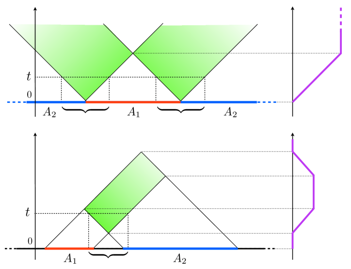
Figure 2: Graphical representation for the quasi-particle spreading of entanglement (for the case with all quasi-particles having the same velocity $v=1$ as in a CFT). The quasi-particles emitted from every point at $t=0$ and reaching one $A_{1}$ (red) and the other $A_{2}$ (blue) are responsible of the entanglement between them. The entanglement at a given time $t$ is proportional to the section of the green shaded area, which is the intersection of the light cones starting from all the points of $A_{1}$ and $A_{2}$ (in the figure these lengths are the braces). The time-dependence of the entanglement obtained in this way are depicted as purple curves on the right for a single interval in the infinite line (top) and two disjoint intervals (bottom): they are proportional to the CFT calculations in Eqs. (24) and (48) respectively. The regions from where the corresponding quasi-particles have been emitted at $t=0$ are obtained by projecting the intersections at time $t=0$ (vertical dashed lines).

4 Quasi-particle interpretation and horizon effect

The time evolution of entanglement and total correlations after a quantum quench can be understood in terms of the quasi-particles interpretation for the propagation of entanglement, first suggested in [10]. According to this argument, since the initial state $|\psi_{0}\rangle$ has a very high energy relative to the ground state of the Hamiltonian which governs the time evolution, it acts as a source of quasi-particle excitations. Particles emitted from points further apart than the correlation length in the initial state are incoherent, but pairs of particles emitted from a given point and subsequently moving to the left or right are highly entangled and correlated. Let us suppose that a pair of quasi-particles with opposite momenta $(p,-p)$ is produced with a probability $\rho(p)$ (which depends on both the Hamiltonian governing the evolution and on the initial state). After their production, these quasi-particles move ballistically with velocity $v_{p}=-v_{-p}$. A quasi-particle of momentum $p$ produced at $x$ is therefore at $x+v_{p}t$ at time $t$. In general there is also a maximum allowed speed of propagation $v_{\rm max}$ (which is connected with the existence of a Lieb-Robinson bound in a lattice model [83]).

Now let us consider two regions of the system $A_{1}$ and $A_{2}$ (which can be either finite, infinite, semi-infinite, etc). According to the argument in [10], the field at some point $x_{1}\in A_{1}$ will be entangled with that at a point $x_{2}\in A_{2}$ if a pair of entangled particles emitted from a point $x$ arrive simultaneously at $x_{1}$ and $x_{2}$. The entanglement and the total correlation between $A_{1}$ and $A_{2}$ are proportional to the length of the interval in $x$ for which this can be satisfied and it can be written as [10]

$${\rm entanglement}\approx\int_{x_{1}\in A_{1}}dx_{1}\int_{x_{2}\in A_{2}}dx_{2}\int_{-\infty}^{\infty}dx\int dp\,\rho(p)f(p)\,\delta(x_{1}-x-v_{p}t)\,\delta(x_{2}-x+v_{p}t)\,,$$ (51)

where $f(p)$ is the contribution of the pair of quasi-particles to the given entanglement or correlation measure.

When all the quasi-particles move with the same speed $|v_{p}|=v$ (as in the case of a CFT discussed in the previous sections where we fixed $v=1$), the $\delta$ functions do not depend on the momentum anymore and therefore the integral over $p$ gives just an overall normalisation (depending on the quantity we are considering), while the integral over the space coordinate can be easily done for arbitrary $A_{1}$ and $A_{2}$. In particular, in the cases of one and two intervals, one straightforwardly recovers all the CFT expressions for the entanglement entropy, mutual information and negativity such as Eqs. (23), (24), (25) and (48). A graphical interpretation of this quasi-particle picture is reported in Fig. 2.

Furthermore, the above argument allows us also to understand what happens in the case of a non-linear dispersion relation leading to a mode dependent velocity, which will be fundamental for the interpretation and the understanding of the numerical data reported in the next section. Indeed, assuming that a maximum speed $v_{\rm max}$ exists, we have that the first linear increase of the entanglement is always present, but when $v_{\rm max}t$ equals the half of some typical length of the configuration given by $A_{1}$ and $A_{2}$, the quasi-particles with velocity smaller than $v_{\rm max}$ start influencing the entanglement because we cannot ignore anymore the integral over $p$ in Eq. (51). These slow quasi-particles lead to non-linear effects discussed e.g. for the entanglement entropy in Refs. [10, 69]. In particular we have that for very long times, the quasi-particles with approximately zero velocity govern the approach to the asymptotic value of the entanglement which usually is power-law as can be easily seen expanding Eq. (51) close to the points where $v_{p}=0$.

It is important to stress at this point that, while it was already established [10, 84, 85] that the mutual information is correctly described by this quasi-particle picture, it is far from obvious that the same reasoning carries over to a complicated measure of the entanglement such as the negativity. The previous section represents a proof of this fact in the context of CFT, while the following one will confirm it also for the harmonic chain.

5 Numerical evaluation of the negativity and mutual information for the harmonic chain

In this section we report the numerical evaluation of the time evolution of entanglement negativity and mutual information after a global quantum quench of the frequency parameter. The Hamiltonian of the periodic harmonic chain with nearest neighbour interactions is

$$H(\omega)=\sum_{s=0}^{L-1}\left(\frac{1}{2m}\,p_{s}^{2}+\frac{m\omega^{2}}{2}\,q_{s}^{2}+\frac{K}{2}(q_{s+1}-q_{s})^{2}\right)\,,\qquad q_{0}=q_{L}\,,\qquad p_{0}=p_{L}\,.$$ (52)

where $L$ is the number of lattice sites of the chain, $m$ a mass scale, $\omega$ the one-particle oscillation frequency, and $K$ a nearest neighbour coupling. The variables $p_{i}$ and $q_{i}$ satisfy standard commutation relations $[q_{i},q_{j}]=[p_{i},p_{j}]=0$ and $[q_{i},p_{j}]=\textrm{i}\delta_{ij}$. We consider the harmonic chain because it is the only lattice model in which the partial transpose and the negativity can be obtained by means of correlation matrix techniques [86, 87]. The model is critical for $\omega=0$ and its continuum limit is conformal with central charge $c=1$. A canonical rescaling of the variables allows to rewrite it in a form where the parameters $\omega$, $m$, $K$ occur only in the global factor and in the coupling between nearest neighbour sites [86, 87]. We consider a quench in the parameter $\omega$, preparing the system in the ground state of (52) with $\omega=\omega_{0}\neq 0$ and letting the system evolve for $t>0$ with the critical Hamiltonian with $\omega=0$. The quench dynamics of the Hamiltonian (52) has been studied already in several papers both on the lattice and in the continuum [9, 88, 89, 90, 91, 92, 93, 94].

The Hamiltonian (52) is simply diagonalised in Fourier space in terms of standard annihilation and creation operators $a_{k}$ and $a_{k}^{\dagger}$. The diagonal form for the Hamiltonian is

$$H(\omega)=\sum_{k=0}^{L-1}\omega_{k}\left(a^{\dagger}_{k}a_{k}+\frac{1}{2}\right)\,,$$ (53)

where the dispersion relation is given by

$$\omega_{k}\equiv\sqrt{\omega^{2}+\frac{4K}{m}\sin^{2}(\pi k/L)}\,\geqslant\omega\,,\qquad k=0,\dots,L-1\,.$$ (54)

Notice that the Hamiltonian has a zero-mode for $k=0$ and $\omega=0$. This usually prevents a straightforward analysis of the critical behaviour, but for the global quench this will not be a problem, as we will see soon. From the dispersion relation, we straightforwardly have the velocity of each momentum mode as

$$v_{k}\equiv\frac{\partial\omega_{k}}{\partial p_{k}}=\,\frac{(K/m)\sin(p_{k})}{\sqrt{\omega^{2}+(4K/m)\sin^{2}(p_{k}/2)}}\,,\qquad p_{k}\equiv\frac{2\pi k}{L}\,,$$ (55)

and the maximum one

$$v_{\rm max}\equiv\textrm{max}_{k}(v_{k})\,,$$ (56)

which determines the spreading of entanglement and correlations. Notice that for $\omega=0$, $v_{\rm max}=1$ for $K=m=1$.

In the quench protocol in which we are interested in, the system is prepared in the ground state $|\psi_{0}\rangle$ of the Hamiltonian

$$H(\omega_{0})=\sum_{k=0}^{L-1}\omega_{0,k}\left(a^{\dagger}_{0,k}a_{0,k}+\frac{1}{2}\right),$$ (57)

whose dispersion relation $\omega_{0,k}$ is Eq. (54) with $\omega=\omega_{0}$. At $t=0$ the frequency parameter is suddenly quenched from $\omega_{0}$ to a different value $\omega$ and the system unitarily evolves through the new Hamiltonian (53), namely

$$|\psi(t)\rangle=e^{-\textrm{i}H(\omega)t}\,|\psi_{0}\rangle\,,\qquad t>0\,.$$ (58)

In order to study the entanglement for the harmonic chain, we need to know the following two-point correlators

$$\begin{array}[]{l}\mathbb{Q}_{r,s}(t)\equiv\langle\psi_{0}|q_{r}(t)q_{s}(t)|\psi_{0}\rangle\,,\\ \rule{0.0pt}{17.07182pt}\mathbb{P}_{r,s}(t)\equiv\langle\psi_{0}|p_{r}(t)p_{s}(t)|\psi_{0}\rangle\,,\\ \rule{0.0pt}{17.07182pt}\mathbb{M}_{r,s}(t)\equiv\langle\psi_{0}|q_{r}(t)p_{s}(t)|\psi_{0}\rangle\,,\end{array}$$ (59)

where $q_{r}(t)$ and $p_{r}(t)$ are the time evolved operators in the Heisenberg picture

$$q_{r}(t)=e^{\textrm{i}Ht}q_{r}(0)e^{-\textrm{i}Ht}\,,\qquad p_{r}(t)=e^{\textrm{i}Ht}p_{r}(0)e^{-\textrm{i}Ht}\,.$$ (60)

These correlators can be written as (see also [93] for a slightly different approach)

$$\mathbb{Q}_{r,s}(t)\;=\;\frac{1}{2L}\sum_{k=0}^{L-1}Q_{k}(t)\cos\Big{[}(r-s)\frac{2\pi k}{L}\Big{]}\,,$$ (61)

$$\mathbb{P}_{r,s}(t)\;=\;\frac{1}{2L}\sum_{k=0}^{L-1}P_{k}(t)\cos\Big{[}(r-s)\frac{2\pi k}{L}\Big{]}\,,$$ (62)

$$\mathbb{M}_{r,s}(t)\;=\;\frac{\textrm{i}}{2}\,\delta_{r,s}-\frac{1}{2L}\sum_{k=0}^{L-1}M_{k}(t)\cos\Big{[}(r-s)\frac{2\pi k}{L}\Big{]}\,,$$ (63)

where we collected the dependence on $\omega$, $\omega_{0}$ and $t$ into

$$Q_{k}(t)\;\equiv\;\frac{1}{m\omega_{k}}\left(\,\frac{\omega_{k}}{\omega_{0,k}}\cos^{2}(\omega_{k}t)+\frac{\omega_{0,k}}{\omega_{k}}\sin^{2}(\omega_{k}t)\right)\,,$$ (64)

$$P_{k}(t)\;\equiv\;m\omega_{k}\left(\,\frac{\omega_{k}}{\omega_{0,k}}\sin^{2}(\omega_{k}t)+\frac{\omega_{0,k}}{\omega_{k}}\cos^{2}(\omega_{k}t)\right)\,,$$ (65)

$$M_{k}(t)\;\equiv\;\left(\,\frac{\omega_{k}}{\omega_{0,k}}-\frac{\omega_{0,k}}{\omega_{k}}\right)\sin(\omega_{k}t)\cos(\omega_{k}t)\,.$$ (66)

We notice that, for $t>0$ and $\omega=0$ the contribution from the mode $k=0$ is finite, indeed

$$Q_{0}(t)\,=\,\frac{1}{m}\left(\,\frac{1}{\omega_{0}}+\omega_{0}t^{2}\right)\,,\qquad P_{0}(t)\,=\,m\omega_{0}\,,\qquad M_{0}(t)\,=\,-\,\omega_{0}t\,.$$ (67)

The other modes are clearly always finite, and so we can consider the global quench to a massless Hamiltonian (while, as well known, we cannot set $\omega=0$ for the equilibrium properties).

From the correlation functions, the entanglement entropy and negativity are constructed by standard methods. Indeed, given a subsystem $A$ of the lattice made by $\tilde{\ell}$ sites which could be either all in one interval or splitted in many disjoint intervals, the reduced density matrix for $A$ can be studied by constructing the $\tilde{\ell}\times\tilde{\ell}$ matrices $\mathbb{Q}_{A}$, $\mathbb{P}_{A}$ and $\mathbb{M}_{A}$, which are the restrictions to the subsystem $A$ of the matrices $\mathbb{Q}$, $\mathbb{P}$ and $\mathbb{M}$ respectively [95, 86, 87, 96]. Given $\mathbb{Q}_{A}$, $\mathbb{P}_{A}$ and $\mathbb{M}_{A}$, the covariance matrix $\gamma_{A}$ associated to the subsystem $A$ and the symplectic matrix $J_{A}$ of the corresponding size are

$$\gamma_{A}(t)\equiv\,\textrm{Re}\begin{pmatrix}\mathbb{Q}_{A}(t)&\mathbb{M}_{A}(t)\\ \mathbb{M}_{A}(t)^{\textrm{t}}&\mathbb{P}_{A}(t)\end{pmatrix},\qquad J_{A}\equiv\begin{pmatrix}\boldsymbol{0}_{\tilde{\ell}}&\mathbb{I}_{\tilde{\ell}}\\ -\mathbb{I}_{\tilde{\ell}}&\boldsymbol{0}_{\tilde{\ell}}\end{pmatrix},$$ (68)

where $\mathbb{I}_{\tilde{\ell}}$ is the $\tilde{\ell}\times\tilde{\ell}$ identity matrix and $\boldsymbol{0}_{\tilde{\ell}}$ is the $\tilde{\ell}\times\tilde{\ell}$ matrix with vanishing elements. We remark that the matrix $\mathbb{M}(t)$ has a non trivial real part for $t>0$. At this point we compute the spectrum of $\textrm{i}J_{A}\cdot\gamma_{A}(t)$ which can be written as $\{\pm\lambda_{a}(t);a=1,\dots\tilde{\ell}\}$ with $\lambda_{a}(t)>0$. The time dependent Rényi entropies as function of the eigenvalues $\lambda_{a}(t)$ are finally written as

$$\textrm{Tr}\,\rho_{A}(t)^{n}=\prod_{a\,=\,1}^{\tilde{\ell}}\left[\bigg{(}\lambda_{a}(t)+\frac{1}{2}\bigg{)}^{n}-\bigg{(}\lambda_{a}(t)-\frac{1}{2}\bigg{)}^{n}\,\right]^{-1},$$ (69)

and the entanglement entropy as

$$S_{A}(t)=\sum_{a\,=\,1}^{\tilde{\ell}}\left[\bigg{(}\lambda_{a}(t)+\frac{1}{2}\bigg{)}\ln\bigg{(}\lambda_{a}(t)+\frac{1}{2}\bigg{)}-\bigg{(}\lambda_{a}(t)-\frac{1}{2}\bigg{)}\ln\bigg{(}\lambda_{a}(t)-\frac{1}{2}\bigg{)}\,\right].$$ (70)

In order to compute the negativity, we denote by $A=A_{1}\cup A_{2}$ a subregion of the harmonic chain and we consider the partial transpose with respect to $A_{2}$. In the covariance matrix $\gamma_{A}$, the net effect of the partial transposition is the inversion of the signs of the momenta corresponding to the sites belonging to $A_{2}$ [86]. Thus, introducing the $\tilde{\ell}\times\tilde{\ell}$ diagonal matrix $\mathbb{R}_{A_{2}}$ which has $-1$ in correspondence of the sites of $A_{2}$ and $+1$ otherwise, we can construct

$$\gamma_{A}^{T_{2}}(t)\equiv\,\begin{pmatrix}\mathbb{I}_{\tilde{\ell}}&\boldsymbol{0}_{\tilde{\ell}}\\ \boldsymbol{0}_{\tilde{\ell}}&\mathbb{R}_{A_{2}}\end{pmatrix}\cdot\gamma_{A}(t)\cdot\begin{pmatrix}\mathbb{I}_{\tilde{\ell}}&\boldsymbol{0}_{\tilde{\ell}}\\ \boldsymbol{0}_{\tilde{\ell}}&\mathbb{R}_{A_{2}}\end{pmatrix},$$ (71)

and compute the spectrum of $\textrm{i}J_{A}\cdot\gamma_{A}^{T_{2}}(t)$, which again can be written as $\{\pm\chi_{a}(t);a=1,\dots\tilde{\ell}\}$ with $\chi_{a}(t)>0$. Then, the trace of the $n$-th power of $\rho_{A}^{T_{2}}$ is

$$\textrm{Tr}(\rho_{A}^{T_{2}})^{n}=\prod_{a\,=\,1}^{\tilde{\ell}}\left[\bigg{(}\chi_{a}(t)+\frac{1}{2}\bigg{)}^{n}-\bigg{(}\chi_{a}(t)-\frac{1}{2}\bigg{)}^{n}\,\right]^{-1},$$ (72)

while the trace norm reads

$$||\rho_{A}^{T_{2}}||=\prod_{a\,=\,1}^{\tilde{\ell}}\Bigg{[}\,\bigg{|}\chi_{a}(t)+\frac{1}{2}\bigg{|}-\bigg{|}\chi_{a}(t)-\frac{1}{2}\bigg{|}\,\Bigg{]}^{-1}=\prod_{a\,=\,1}^{\tilde{\ell}}\textrm{max}\bigg{[}1,\frac{1}{2\chi_{a}(t)}\bigg{]}\,,$$ (73)

which gives the logarithmic negativity $\mathcal{E}=\ln(||\rho_{A}^{T_{2}}||)$.

In what follows we will compute entanglement entropies and negativity from the above formulas by calculating the spectrum of the appropriate covariance matrix. Since the parameters $K$ and $m$ can be absorbed in a redefinition of the canonical variables, we fix them to $K=m=1$ and we just consider a quench in the frequency (or mass) parameter from $\omega_{0}$ to $\omega$. The data obtained by numerically diagonalising the covariance matrix for several bi- and tripartitions of the harmonic chain are reported in the following subsections.

5.1 The entanglement entropy of one interval

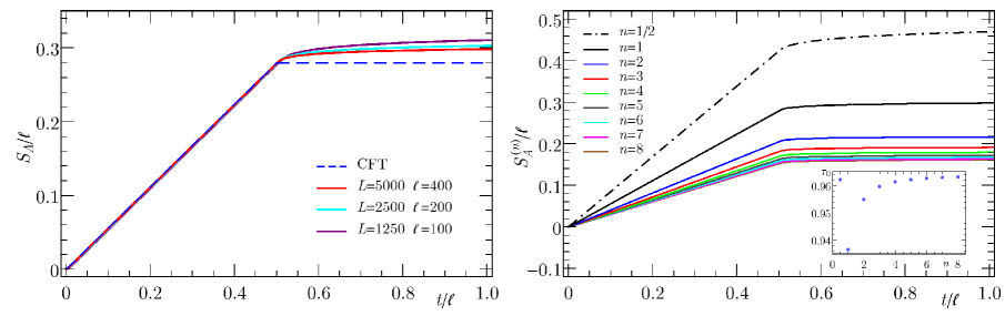
Figure 3: Left: Temporal evolution of the entanglement entropy for one interval of $\ell$ sites in a periodic harmonic chain with $L$ sites. At $t=0$ the mass is quenched from $\omega_{0}=1$ to $\omega=0$. The dashed curve is the CFT prediction (24) with $c=1$ and the best fitted value for $\tau_{0}$. Right: Temporal evolution of the Rényi entropies and of the logarithmic negativity $\mathcal{E}_{A}$, which coincides with $S_{A}^{(1/2)}$ in this case, for a periodic chain with $L=5000$ and $\ell=400$. In the inset, we report the best fitted values of $\tau_{0}$ for the values of $n$ displayed in the main plot.

It is instructive to start our analysis from the study of the quench dynamics of the entanglement entropy of a single interval, although this has been recently studied in Ref. [93]. Indeed, this preliminary analysis allows us to understand the regime of applicability of the CFT and the optimal quench parameters in order to observe a CFT scaling.

In Fig. 3, we report the time evolution of the entanglement entropy for a quench from $\omega_{0}=1$ to $\omega=0$. We consider finite chains of length up to $L=5000$ and several values of $\ell\ll L$ with $\ell/L$ kept fixed. It is evident from the figure that the behaviour of von Neumann and Rényi entropy is in good qualitative agreement with the CFT prediction (24) with a linear growth for $t<\ell/2$ followed by saturation for $t>\ell/2$ (we recall that for $\omega=0$ the maximum mode velocity is $v_{\rm max}=1$, cf. Eq. (56)). However, few comments on these results are needed. First, for $t>\ell/2$ the entanglement entropies do not saturate but they show a slow growth toward an asymptotic value. This is a well known phenomenon [10, 69] and it is due to the entanglement generated by slow quasi-particles moving with velocity $v_{k}<v_{\rm max}=1$ as in Eq. (55). A second comment concerns the fitted value of $\tau_{0}$: this is shown in the inset of Fig. 3 as function of the order of the Rényi entropy $n$. There is a minor dependence on $n$, as already anticipated and noticed in the literature [93], but overall $\tau_{0}$ is very close to the initial correlation length $\xi_{0}\sim\omega_{0}^{-1}=1$. Finally we must comment on the chosen value of $\omega_{0}=1$. In preliminary calculations we considered several values of $\omega_{0}$ which however we do not report here, but $\omega_{0}=1$ is the one for which the conformal scaling describes the data more accurately. This can be easily understood from the fact that (i) we should be in the regime $t,\ell\gg\omega_{0}^{-1}$ requiring that the initial frequency should not be too small, (ii) we should be in a regime in which the continuum description is appropriate, requiring the initial correlation length not to be too small (i.e. $\omega_{0}$ not too large), in order to avoid a magnification of lattice effects. The value $\omega_{0}\sim 1$ appears to be the best compromise between these two effects.

The Rényi entropy with $n=1/2$ corresponds to the logarithmic negativity, but, as expected, does not display any peculiar behaviour compared with the other values of $n$.

5.2 Two adjacent intervals

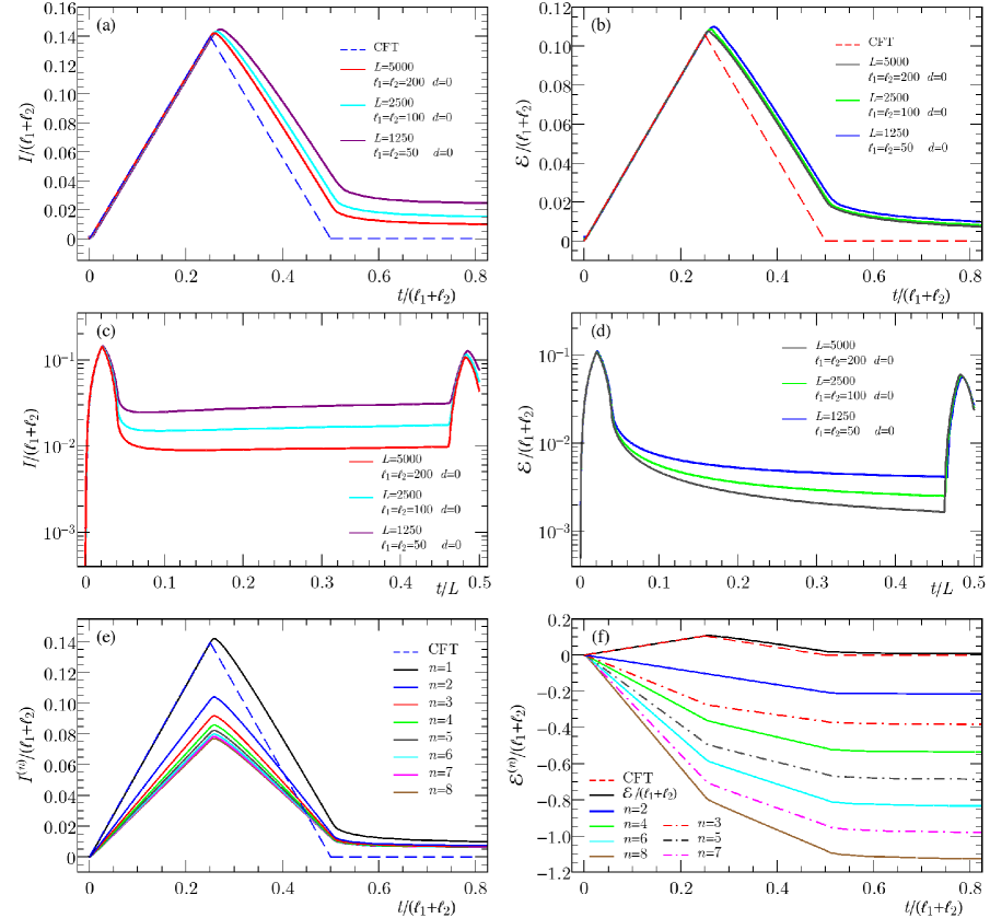
Figure 4: Adjacent intervals with several equal lengths $\ell_{1}=\ell_{2}$ and for various total size $L$ of the periodic harmonic chain. All panels show the data for $\omega_{0}=1$ and a critical evolution, $\omega=0$. Panels (a) and (c) display the mutual information $I$ while (b) and (d) the logarithmic negativity $\mathcal{E}$. Top and middle panels show different time scales and the revivals due to the finiteness of the system are evident in the middle panels, where a larger range of $t$ is considered. The dashed CFT curves in (a) and (b) are given by (26) and (41) respectively. In the last two panels we show the time evolution of the Rényi mutual information $I^{(n)}$ (e) and of the replicated negativity $\mathcal{E}^{(n)}$ (f) for various values of $n$.

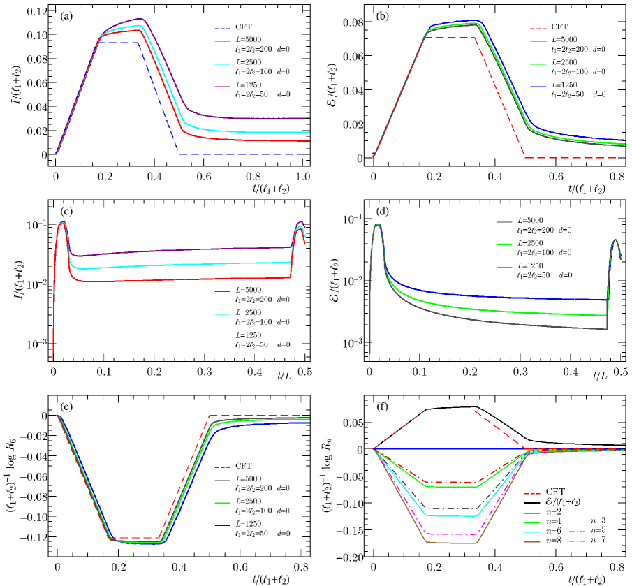
Figure 5: Adjacent intervals with different lengths $\ell_{1}=2\ell_{2}$ for different intervals lengths and total size $L$ of the periodic harmonic chain. Critical evolution of the mutual information $I$ (panel (a), (c)) and of the logarithmic negativity $\mathcal{E}$ (panels (b), (d)). The revivals are reported in panels (c) and (d). Notice that outside the light cone $\mathcal{E}$ always decays while $I$ reaches a plateau (apart from some finite size effects responsible of a very slow increase) (panels (c) and (d)). Compared to Fig. 4 for the case of intervals with equal length, we observe a plateau starting at $t\simeq\textrm{min}(\ell_{1},\ell_{2})/2$ with temporal width $|\ell_{2}-\ell_{1}|/2$. The panel (e) and (f) report the ratios $R_{n}$ for several values of $n$.

We start the study of the entanglement between two different intervals from the case of adjacent ones. In the various figures that will follow we report both the mutual information and the negativity in order to simplify the discussion of similarity and differences. As already stressed above, the principal new results of this manuscript concern the evaluation of the negativity, since the time dependence of the mutual information in CFT was already established in [10] and these results were checked in a few numerical works for the Ising chain [85] and the Bose-Hubbard model [84], but, to the best of our knowledge, not for the harmonic chain.

The numerical results for two adjacent intervals for a quench from $\omega_{0}=1$ to $\omega=0$ are shown in Figs. 4 and 5. The main differences between the two sets of plots is that in the first one the two intervals have equal lengths, while in the second one the length of one interval is half of the other. Let us discuss these two sets of plots critically. In the top panels of Fig. 4, we report the time evolution of the mutual information (a) and logarithmic negativity (b) on time scales of the order of $\ell$. They have a very similar behaviour characterised by an initial linear growth, followed by an almost linear dropping up to time $t=\ell_{1}$ when a slow power-law relaxation to the asymptotic vanishing value starts. These results are in agreement with the expectation from CFT and their behaviour is simply understood in terms of the quasi-particle picture as already explained in Sec. 4. Also the differences between the linear CFT behaviour and the non-linear one of the actual data is easily understood in terms of the slow quasi-particles in analogy to the entanglement entropy of a single interval in the previous subsection. No particular difference is observed in this regime between negativity and mutual information. In the two middle panels of Fig. 4, we again report the time evolution of the mutual information (c) and logarithmic negativity (d), but on time scales of the order of the system’s size $L$. The main feature in this case is the presence of quantum revivals at time equal to $t\simeq(L-[\ell_{1}+\ell_{2}])/2$. A first important difference between the mutual information and the negativity appears on these time-scales, indeed while the former reaches a plateau in a large time-window, the latter decreases monotonically until the revival. Finally, in the last two panels we also report the Rényi mutual information (e) and the replicated negativity ${\cal E}^{(n)}$. Their behaviour is again in qualitative agreement with the CFT predictions and the differences are easily understood in terms of slow quasi-particles. However, we mention that ${\cal E}^{(n)}$ with $n>1$ does not follow the same behaviour as the mutual information or negativity and indeed it is a monotonically decreasing function of time, changing the slope in the time intervals identified above (i.e. at $t=\ell_{1}/2$ and at $t=\ell_{1}$). This is not a surprise since ${\cal E}^{(n)}$ is not a measure of entanglement and neither a quantifier of the correlations. However, as already stressed, the piece-wise quasi-linear behaviour is compatible with the CFT prediction apart from the effect of the slow modes.

In Fig. 5, we report the case of two adjacent intervals of different lengths $\ell_{1}=2\ell_{2}$. The main difference compared to the case of equal lengths is the appearance of a plateau after the first linear increase for both the mutual information and the negativity. This is in perfect agreement with the CFT results which indeed predict (see Eqs. (26) and (41)) a linear increase up to $t={\rm min}(\ell_{1},\ell_{2})/2$, followed by a plateau for ${\rm min}(\ell_{1},\ell_{2})/2<t<{\rm max}(\ell_{1},\ell_{2})/2$, a linear decrease for ${\rm max}(\ell_{1},\ell_{2})/2<t<(\ell_{1}+\ell_{2})/2$, and finally zero constantly. It is evident that the differences between CFT and actual data for the harmonic chain are due to slow quasi-particles which give corrections for $t>{\rm min}(\ell_{1},\ell_{2})/2$. In the panel (c) and (d) of Fig. 5 we show the evolution of mutual information and negativity for a larger time window and, as before, the revivals are apparent at time $t=(L-\ell_{1}-\ell_{2})/2$. Finally in the last two panels (e) and (f) we report the behaviour of the universal ratio $R_{n}$ as a function of time. Again there are no particular differences with the CFT prediction except for those ones due to slow quasi-particles. From the last panel (f), one notices that $R_{2}=1$ identically. In the quantum field theory approach, this exceptional behaviour for $n=2$ is easily understood from the fact that $\mathcal{T}^{2}_{2}=\bar{\mathcal{T}}^{2}_{2}=\mathbb{I}$ (cf. Sec. 3.3) and it is true also on the lattice. Notice that $\ln(R_{n})$ has a behaviour which closely resembles the one of the mutual information and the negativity, showing that, in this particular case, they are somehow measuring the amount of correlations or entanglement. This is an important difference compared to the quantity ${\cal E}^{(n)}$ in Fig. 4.

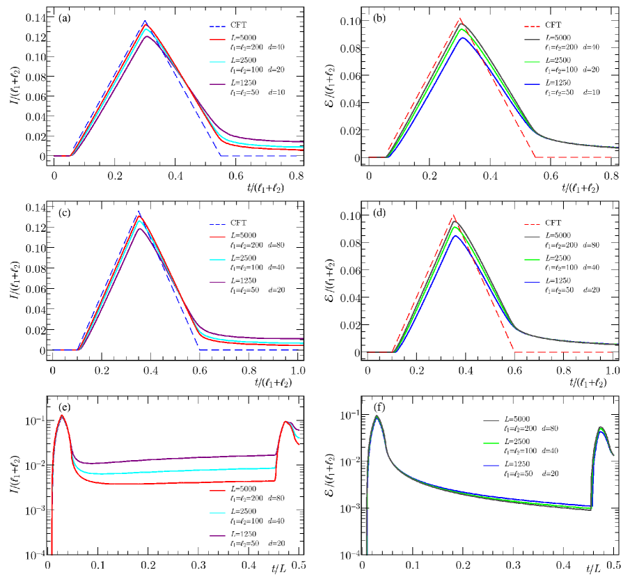
Figure 6: Disjoint intervals with equal lengths $\ell_{1}=\ell_{2}$ separated by $d$ sites, for various intervals lengths, separations $d$, and total size $L$ of the periodic harmonic chain. Time evolution of the mutual information $I$ ((a), (c) and (e)) and of the logarithmic negativity $\mathcal{E}$ ((b), (d), and (f)). The revivals at large $t$ are evident in the bottom panels.

5.3 Two disjoint intervals

In this subsection we move to the case of two disjoint intervals. In Fig. 6 we report the numerically calculated mutual information and negativity for two disjoint intervals of equal length and for two different sets of distances between them. It is clear from the figure that the main difference compared to the case of adjacent interval is that there is an initial region for $t<d/2$ in which there is no entanglement and no correlations (we recall that the initial correlation length is $\omega_{0}^{-1}=1$, so that the initial entanglement is very small). Then at time equal to $d/2$ the entanglement starts growing linearly, reaches a maximum and then decreases almost linearly. Again, this behaviour is compatible with the quasi-particle interpretation and also the power law relaxation for large times can be understood in terms of slow modes. Even in the case of disjoint intervals, we have studied the revivals. The results, which are very similar to the ones shown in the case of adjacent intervals, are reported in Fig. 6, panels (e) and (f).

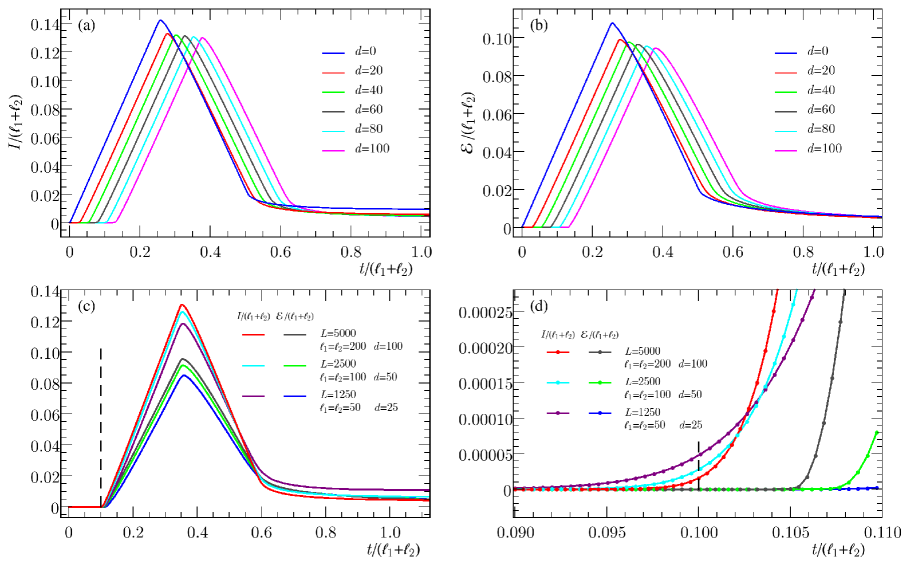
Figure 7: Mutual information (a) and the logarithmic negativity (b) of disjoint intervals with equal lengths $\ell_{1}=\ell_{2}=200$, separated by distances $d$ in a periodic chain with $L=5000$. (c) Comparison between $I$ and $\mathcal{E}$. (d) Zoom of the initial growth: a late birth effect for $\mathcal{E}$ is observed, which decreases as the continuum limit is approached. The vertical dashed line in (c) and (d) indicates the time $t=d/2$ where the growth should start in the continuum theory.

Conversely, a very interesting phenomenon can be observed by looking at very short times after the entanglement starts growing. This is illustrated in Fig. 7, where in the top panels we show the mutual information and the negativity as function of time for different distances between the two intervals. As before, the behaviour is very reminiscent of the CFT prediction. In the panel (c) of the same figure, we show in the same plot the negativity and the mutual information for fixed $d/\ell$ and looking closely to the time when the entanglement starts growing it is already clear that something is happening. For this reason in the panel (d) we zoom close to the point $t=d/2$ and we highlight a very peculiar phenomenon: while the mutual information starts moving from zero slightly before $t=d/2$ the negativity starts slightly after $t=d/2$. The behaviour of the mutual information is simply the exponential tails of the correlations outside the light-cone, but the behaviour of the negativity is new. From the figure, it is evident that increasing the total system size $L$ (at fixed ratios $d/L$ and $\ell/L$) this phenomenon disappears in such a way to recover the CFT result and the quasi-particle interpretation of the evolution in the continuum limit. As a consequence, this remarkable phenomenon is a lattice effect and so cannot have an explanation in terms of quasi-particles, but it would be interesting to understand its precise origin. In a suggestive way, and in analogy with the famous sudden death of entanglement [97] (which will be discussed below), we term this phenomenon as the late birth of entanglement.

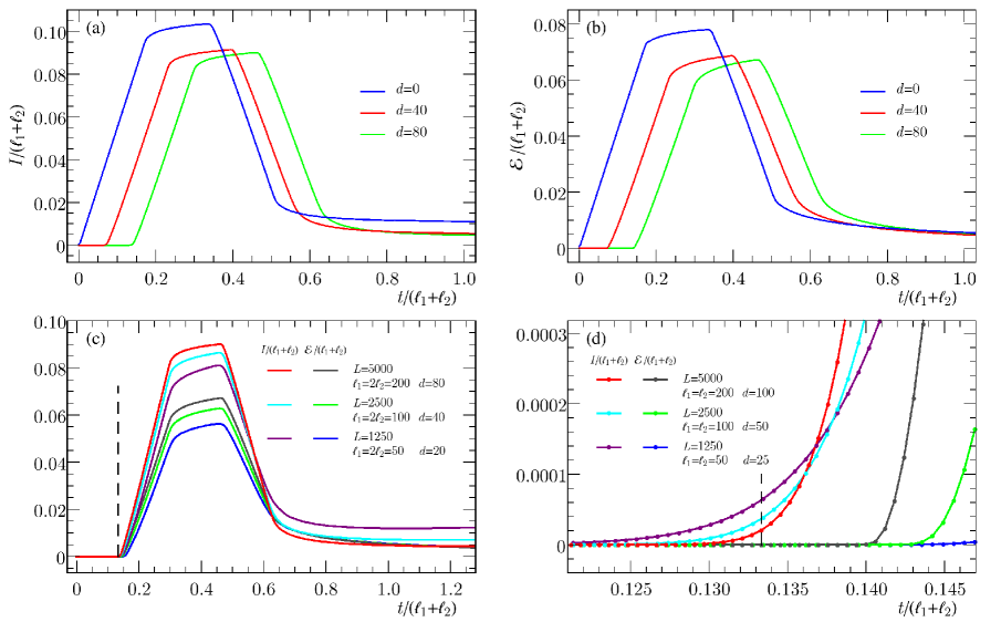
Figure 8: Mutual information (a) and the logarithmic negativity (b) of disjoint intervals with different lengths $\ell_{1}=2\ell_{2}=200$, separated by various distances $d$ sites in a periodic chain with $L=5000$. Comparison between $I$ and $\mathcal{E}$ in (c) and zoom on the initial growth in (d), to highlight the late birth of $\mathcal{E}$. With respect to the corresponding plots in Fig. 7, here a plateau occurs whose temporal width is $|\ell_{2}-\ell_{1}|/2$. The vertical dashed line in (c) and (d) indicates the time $t=d/2$ where the growth should begin, according to the quasi-particles picture.

In Fig. 8 we consider again the mutual information (a) and the negativity (b) for various distances between two intervals of different lengths $\ell_{1}=2\ell_{2}$. The behaviour is in perfect agreement with the CFT prediction with a linear growth starting at $d/2$ up to $d/2+\textrm{min}(\ell_{1},\ell_{2})/2$, followed by a plateau lasting $|\ell_{1}-\ell_{2}|/2$, then a linear decrease up to $t=(d+\ell_{1}+\ell_{2})/2$ and finally a power-law approach to zero. In the panel (c) we report on the same plot the negativity and the mutual information, observing again the fingerprints of the late birth, which are straightforwardly confirmed by zooming for times close to $d/2$, as done in panel (d).

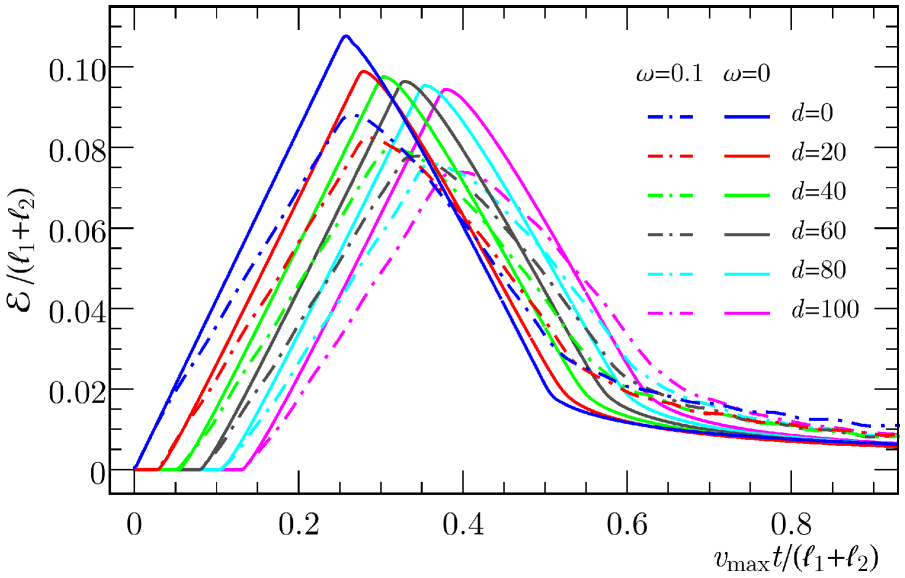
Figure 9: Logarithmic negativity $\mathcal{E}$ of disjoint intervals after global quenches with different evolution Hamiltonians. Here $L=5000$, $\ell_{1}=\ell_{2}=200$ and $\omega_{0}=1$, while for $t>0$ we have $\omega=0$ or $\omega=0.1$. The velocity $v_{\rm max}$ is given by Eq. (56).

5.4 Massive evolution

In this section we briefly discuss what happens when the time evolution is governed by a massive Hamiltonian. This is elucidated with an example in Fig. 9 where we report and compare critical ($\omega=0$) and noncritical ($\omega=0.1$) evolution of the logarithmic negativity always starting from $\omega_{0}=1$. The data are reported against $v_{\rm max}t$ ($v_{\rm max}$ is given by Eq. (56)). Also in this case, the data are perfectly compatible with the quasi-particle picture, but we notice an interesting effect. The slope of the negativity changes as a function of time as a consequence of the entanglement carried by slower quasi-particles which in the case of the non-critical evolution have a larger weight because of the non-monotonicity of $v_{k}$ in Eq. (55). However, also this phenomenon does not come as a surprise and indeed it was already observed for the entanglement entropy of a single interval following a quench in the Ising/XY chain [69, 24].

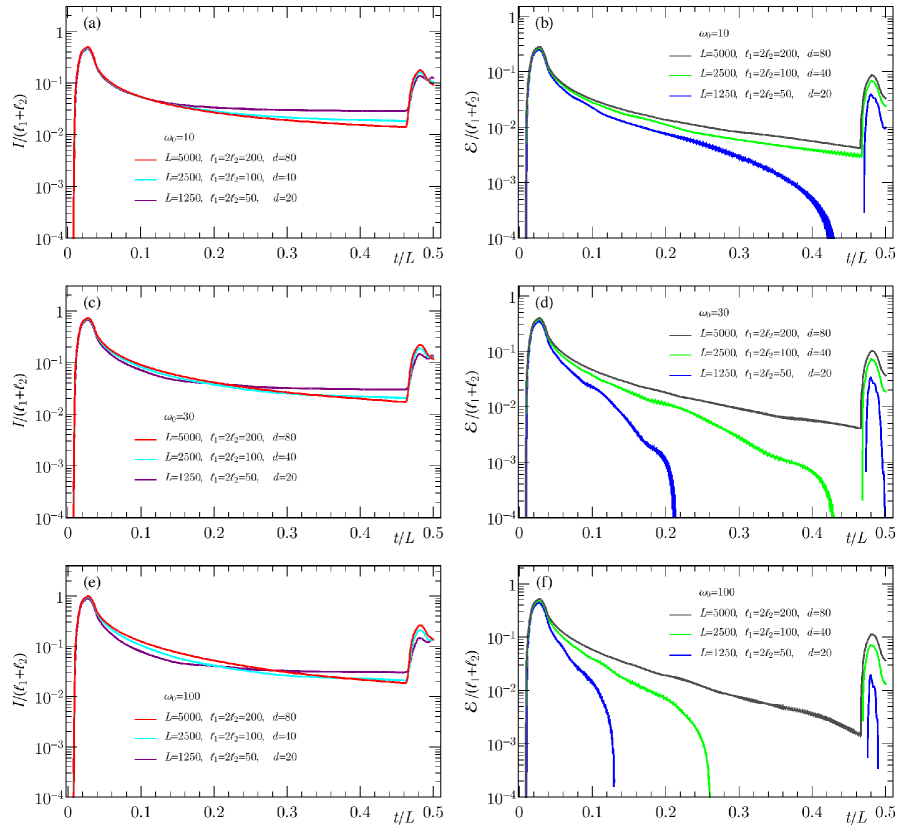
Figure 10: Mutual information (left panels) and logarithmic negativity (right panels) for disjoint intervals with different lengths ($\ell_{1}=2\ell_{2}$). Here $\omega=0$ and different $\omega_{0}$ are chosen: $\omega_{0}=10$, $\omega_{0}=30$ and $\omega_{0}=100$ (top, middle and bottom panels respectively). The sudden death of the logarithmic negativity happens for later time as $L$ increases and as $\omega_{0}$ decreases.

5.5 Sudden death of entanglement

A final important feature of the logarithmic negativity $\mathcal{E}$ is the so called sudden death of entanglement. The phenomenon has been first introduced for other entanglement measures [97], but it has been observed also for the negativity. For example, in the case of the harmonic chain at thermal equilibrium at some finite $T$, it consists into the exact vanishing of $\mathcal{E}$ for temperatures larger than a critical value as discussed also in [15, 81, 82], where it was emphasised its lattice nature and its absence in the quantum field theory description of the continuum limit. In the case of quench, we have already seen that the entanglement and the mutual information of two intervals are vanishing for large enough time in the CFT, but this is an independent phenomenon compared to the sudden death.

In order to show the true sudden death of $\mathcal{E}$ after a global quench, we report in Fig. 10 the negativity and we compare it to the mutual information for several initial frequencies $\omega_{0}=10$, $\omega_{0}=30$ and $\omega_{0}=100$ and for several configurations of the intervals. It is evident that in all cases, while the mutual information stays finite at any time, the negativity $\mathcal{E}$ drops suddenly to zero after some time. Thus, the sudden death is a peculiarity of the entanglement and it is not reflected by the correlations (quantified by the mutual information) which are always a smooth function of the time. Let us now discuss how this phenomenon depends on the various parameters. First, we notice that increasing the system size and keeping the ratios between the various lengths fixed, the sudden death time increases and, when the system and the subsystems are large enough, the sudden death does not occur anymore. This agrees with the expectation that the sudden death is a lattice effect. Second we observe that the sudden death depends also on the initial frequency $\omega_{0}$: increasing $\omega_{0}$, the sudden death time decreases. Finally, it is worth noticing that, when the revival takes place, the entanglement appears again, but this is not at all surprising.

6 Conclusions

We studied the evolution of the entanglement negativity following a quantum quench. We considered the case of a conformal evolution starting from a boundary state. First, for the sake of completeness, we reviewed the results for the entanglement entropy and the mutual information of an arbitrary number of (adjacent or disjoint) intervals within the path integral approach of Refs. [10, 3, 9]. Then we moved to the calculation of the negativity between two adjacent and disjoint intervals which are respectively given by Eqs. (41) and (48). The applicability and generality of these results have been checked against exact numerical calculations for the same quantities in the harmonic chain. One of the main results of this study is that the quasi-particle picture [10] for the time dependence of the entanglement after a global quantum quench applies also to the negativity between two intervals: this is a remarkable and non-trivial property. We also highlight two peculiar lattice effects: the late birth of entanglement and its sudden death. The former one consists in the fact that the negativity starts growing slightly after the time predicted by the quasi-particle picture, a delay which vanishes in the continuum limit. The latter one, instead, is well known and concerns the exact vanishing of the negativity after some given large time (but before revivals take place). We investigated how these effects depend on the quench parameters.

While we draw a quite complete picture for the evolution of the negativity after a quantum quench, there are still some questions deserving further investigations. First, it would be very interesting to obtain analytical forms in the harmonic chain for the evolution of the various entanglement measures (entropy, mutual information, and negativity) in analogy to what done in Refs. [69, 85, 98] for the Ising model (but only for entropy and mutual information). However, we should stress that there are still no analytic results for the entanglement entropy of bosonic models even in the ground state, in contrast with the many results available for free fermion thanks to Toeplitz matrix techniques [99, 100, 101, 102]. Obtaining such analytic predictions is a prerequisite in order to tackle the quench problem.

References

References

- [1] A. Polkovnikov, K. Sengupta, A. Silva, and M. Vengalattore, Rev. Mod. Phys. 83, 863 (2011).
- [2] J. Eisert, M. Friesdorf, and C. Gogolin, arXiv:1408.5148.
- [3] P. Calabrese and J. Cardy, Phys. Rev. Lett. 96, 136801 (2006).
- [4] J.-S. Caux and F. H. L. Essler, Phys. Rev. Lett. 110, 257203 (2013).
- [5] D. Iyer and N. Andrei, Phys. Rev. Lett. 109, 115304 (2012).
-
[6]
A. J. Daley, C. Kollath, U. Schollwoeck, and G. Vidal,
J. Stat. Mech. P04005 (2004);
S. R. White and A. E. Feiguin, Phys. Rev. Lett. 93, 076401 (2004). - [7] G. Vidal, Phys. Rev. Lett. 98, 070201 (2007).
- [8] U. Schollwoeck, Ann. Phys. 326, 96 (2011).
- [9] P. Calabrese and J. Cardy, J. Stat. Mech. P06008 (2007).
- [10] P. Calabrese and J. Cardy, J. Stat. Mech. P04010 (2005).
- [11] J. Cardy, Phys. Rev. Lett. 112, 220401 (2014).
- [12] M. Cheneau, P. Barmettler, D. Poletti, M. Endres, P. Schauss, T. Fukuhara, C. Gross, I. Bloch, C. Kollath, and S. Kuhr, Nature 481, 484 (2012).
- [13] P. Calabrese, J. Cardy, and E. Tonni, Phys. Rev. Lett. 109, 130502 (2012).
- [14] P. Calabrese, J. Cardy, and E. Tonni, J. Stat. Mech. (2013) P02008.
- [15] P. Calabrese, J. Cardy, and E. Tonni, arXiv:1408.3043.
- [16] V. Eisler and Z. Zimboras, arXiv:1406.5474.
- [17] M. Hoogeveen and B. Doyon, Entanglement negativity and entropy in non-equilibrium conformal field theory, to appear.
- [18] S. Sotiriadis and J. Cardy, J. Stat. Mech. (2008) P11003.
-
[19]
A. Gambassi and A. Silva, Phys. Rev. Lett. 109, 250602 (2012);
A. Gambassi and A. Silva, arXiv:1106.2671 - [20] M. Marcuzzi and A. Gambassi, Phys. Rev. B 89, 134307 (2014).
-
[21]
M. Nozaki, T. Numasawa, and T. Takayanagi, Phys. Rev. Lett. 112, 111602 (2014);
M. Nozaki, JHEP 1410 (2014) 147. - [22] P. Calabrese and J. Cardy, J. Stat. Mech. P10004 (2007).
-
[23]
V. Eisler and I. Peschel, J. Stat. Mech. (2007) P06005;
V. Eisler, D. Karevski, T. Platini, and I. Peschel, J. Stat. Mech. (2008) P01023. - [24] J.-M. Stéphan and J. Dubail, J. Stat. Mech. (2011) P08019.
-
[25]
V. Eisler and I. Peschel, EPL 99, 20001 (2012);
M. Collura and P. Calabrese, J. Phys. A 46, 175001 (2013). - [26] J. Cardy, Phys. Rev. Lett. 106, 150404 (2011).
- [27] C. T. Asplund and A. Bernamonti, Phys. Rev. D 89, 066015 (2014).
-
[28]
L. Amico, R. Fazio, A. Osterloh, and V. Vedral, Rev. Mod. Phys. 80, 517 (2008);
J. Eisert, M. Cramer, and M. B. Plenio, Rev. Mod. Phys. 82, 277 (2010);
P. Calabrese, J. Cardy, and B. Doyon Eds, J. Phys. A 42 500301 (2009). - [29] P. Calabrese and A. Lefevre, Phys. Rev. A 78, 032329 (2008).
- [30] M. M. Wolf, F. Verstraete, M.B. Hastings, and I. J. Cirac, Phys. Rev. Lett. 100, 070502 (2008).
-
[31]
G. Vidal and R. F. Werner, Phys. Rev. A 65, 032314 (2002);
G. Vidal, J. Mod. Opt. 47 (2000) 355. -
[32]
K. Zyczkowski, P. Horodecki, A. Sanpera and M. Lewenstein,
Phys. Rev. A 58, 883 (1998);
A. Peres, Phys. Rev. Lett. 77, 1413 (1996). -
[33]
J. Eisert, quant-ph/0610253;
J. Eisert and M. B. Plenio, J. Mod. Opt. 46, 145 (1999). - [34] H. Wichterich, J. Molina-Vilaplana, and S. Bose, Phys. Rev. A 80, 010304 (2009).
- [35] S. Marcovitch, A. Retzker, M. B. Plenio, and B. Reznik, Phys. Rev. A 80, 012325 (2009).
- [36] H. Wichterich, J. Vidal, and S. Bose, Phys. Rev. A 81, 032311 (2010).
-
[37]
A. Bayat, P. Sodano, and S. Bose,
Phys. Rev. Lett. 105, 187204 (2010);
A. Bayat, P. Sodano, and S. Bose, Phys. Rev. B 81, 064429 (2010);
P. Sodano, A. Bayat, and S. Bose, Phys. Rev. B 81, 100412 (2010);
A. Bayat, S. Bose, P. Sodano, and H. Johannesson, Phys. Rev. Lett. 109, 066403 (2012). -
[38]
R. Santos, V. Korepin, and S. Bose,
Phys. Rev. A 84, 062307 (2011);
R. Santos and V. Korepin, J. Phys. A 45, 125307 (2012). - [39] H. He and G. Vidal, arXiv:1401.5843.
- [40] P. Calabrese, C. Hagendorf, P. Le Doussal, J. Stat. Mech. (2008) P07013.
- [41] J. Cardy, Quantum quenches in perturbed conformal field theory, talk GGI workshop “New non-equilibrium states of matter in and out of equilibrium”, May 2012.
- [42] S. Sotiriadis and J. Cardy, Phys. Rev. B 81, 134305 (2010).
- [43] A. Gambassi and P. Calabrese, EPL 95 (2011) 66007.
- [44] S. Sotiriadis, G. Takacs, and G. Mussardo, Phys. Lett. B 734, 52 (2014).
-
[45]
D. Fioretto and G. Mussardo,
New J. Phys. 12, 055015 (2010);
S. Sotiriadis, D. Fioretto, and G. Mussardo, J. Stat. Mech. (2012) P02017. - [46] P. Calabrese and J. Cardy, J. Stat. Mech. P06002 (2004).
- [47] P. Calabrese and J. Cardy, J. Phys. A 42, 504005 (2009).
- [48] J. L. Cardy, O.A. Castro-Alvaredo, and B. Doyon, J. Stat. Phys. 130 (2008) 129.
- [49] V. G. Knizhnik, Commun. Math. Phys. 112, (1987) 567.
- [50] M. Caraglio and F. Gliozzi, JHEP 0811: 076 (2008).
- [51] S. Furukawa, V. Pasquier, and J. Shiraishi, Phys. Rev. Lett. 102, 170602 (2009).
- [52] P. Calabrese, J. Cardy, and E. Tonni, J. Stat. Mech. P11001 (2009).
- [53] P. Calabrese, J. Cardy, and E. Tonni, J. Stat. Mech. P01021 (2011).
- [54] F. Igloi and I. Peschel, 2010 EPL 89 40001.
- [55] P. Calabrese, J. Stat. Mech. (2010) P09013.
-
[56]
H. Casini and M. Huerta,
Class. Quant. Grav. 26, 185005 (2009);
H. Casini, J. Stat. Mech. (2010) P08019;
D. D. Blanco and H. Casini, Class. Quant. Grav. 28, 215015 (2011). - [57] V. Alba, L. Tagliacozzo, and P. Calabrese, Phys. Rev. B 81 060411 (2010).
- [58] V. Alba, L. Tagliacozzo, and P. Calabrese, J. Stat. Mech. (2011) P06012.
- [59] M. Headrick, Phys. Rev. D 82, 126010 (2010).
- [60] M. A. Rajabpour and F. Gliozzi, J. Stat. Mech. (2012) P02016.
- [61] M. Fagotti, EPL 97, 17007 (2012).
- [62] B. Chen and J. Zhang, JHEP 1311 (2013) 164.
- [63] A. Coser, L. Tagliacozzo, and E. Tonni, J. Stat. Mech. (2014) P01008.
-
[64]
S. Ryu and T. Takayanagi,
Phys. Rev. Lett. 96 (2006) 181602;
S. Ryu and T. Takayanagi, JHEP 0608: 045 (2006);
V. E. Hubeny and M. Rangamani, JHEP 0803: 006 (2008);
M. Headrick and T. Takayanagi, Phys. Rev. D 76, 106013 (2007);
T. Nishioka, S. Ryu, and T. Takayanagi, J. Phys. A 42 (2009) 504008;
E. Tonni, JHEP 1105:004 (2011);
J. Molina-Vilaplana and P. Sodano, JHEP 10 (2011) 011;
M. Headrick, A. Lawrence, and M. M. Roberts, J. Stat. Mech. (2013) P02022;
I. A. Morrison and M. M. Roberts, JHEP 07 (2013) 081;
T. Faulkner, arXiv:1303.7221;
T. Hartman, arXiv:1303.6955;
T. Faulkner, A. Lewkowycz, and J. Maldacena, JHEP 1311 (2013) 074. - [65] J. Cardy, J. Phys. A 46 (2013) 285402.
- [66] H. Casini and M. Huerta, JHEP 0903: 048 (2009).
- [67] N. Shiba, Phys. Rev. D 83, 065002 (2011); N. Shiba, JHEP 1207:100 (2012); N. Shiba, arXiv:1408.0637.
- [68] H. J. Schnitzer, arXiv:1406.1161.
- [69] M. Fagotti and P. Calabrese, Phys. Rev. A 78, 010306 (2008).
- [70] P. Calabrese, F. H. L. Essler, and M. Fagotti, Phys. Rev. Lett. 106, 227203 (2011).
-
[71]
P. Calabrese, F. H. L. Essler, and M. Fagotti, J. Stat. Mech. (2012) P07016;
P. Calabrese, F. H. L. Essler, and M. Fagotti, J. Stat. Mech. (2012) P07022. -
[72]
V. Balasubramanian, A. Bernamonti, J. de Boer, N. Copland, B. Craps, E. Keski-Vakkuri, B. Muller, A. Schafer,
M. Shigemori, and W. Staessens,
Phys. Rev. Lett. 106 (2011) 191601;
V. Balasubramanian, A. Bernamonti, J. de Boer, N. B. Copland, B. Craps, E. Keski-Vakkuri, B. Muller, A. Schafer, M. Shigemori and W. Staessens, Phys. Rev. D 84 (2011) 026010;
A. Buchel, L. Lehner, R. C. Myers, and A. van Niekerk, JHEP 1305 (2013) 067;
M. J. Bhaseen, J. P. Gauntlett, B. D. Simons, J. Sonner, and T. Wiseman, Phys. Rev. Lett. 110 (2013) 015301. -
[73]
V. E. Hubeny, M. Rangamani, and T. Takayanagi,
JHEP 0707 (2007) 062;
J. Abajo-Arrastia, J. Aparicio, and E. Lopez, JHEP 1011 (2010) 149;
J. Aparicio and E. Lopez, JHEP 1112 (2011) 082;
V. Balasubramanian, A. Bernamonti, N. Copland, B. Craps, and F. Galli, Phys. Rev. D 84 (2011) 105017;
A. Allais and E. Tonni, JHEP 1201 (2012) 102;
R. Callan, J. Y. He, and M. Headrick, JHEP 1206 (2012) 081;
T. Hartman and J. Maldacena, JHEP 1305 (2013) 014;
H. Liu and S. J. Suh, Phys. Rev. D 89 (2014) 066012;
H. Liu and S. J. Suh, Phys. Rev. Lett. 112 (2014) 011601. - [74] V. Alba, J. Stat. Mech. P05013 (2013).
- [75] P. Calabrese, L. Tagliacozzo and E. Tonni, J. Stat. Mech. P05002 (2013).
- [76] M. Rangamani and M. Rota, JHEP 1410 (2014) 60
- [77] M. Kulaxizi, A. Parnachev, and G. Policastro, JHEP 1409 (2014) 010.
-
[78]
C. Castelnovo, Phys. Rev. A 88, 042319 (2013);
C. Castelnovo, Phys. Rev. A 89, 042333 (2014). - [79] Y. A. Lee and G. Vidal, Phys. Rev. A 88, 042318 (2013).
- [80] C.-M. Chung, V. Alba, L. Bonnes, P. Chen, A. M. Lauchli, Phys. Rev. B 90, 064401 (2014).
-
[81]
J. Anders and A. Winter,
Quantum Inf. Comput. 8, 0245 (2008);
J. Anders, Phys. Rev. A 77, 062102 (2008). -
[82]
A. Ferraro, D. Cavalcanti, A. Garcia-Saez, and A. Acin,
Phys. Rev. Lett. 100, 080502 (2008);
D. Cavalcanti, A. Ferraro, A. Garcia-Saez, and A. Acin, Phys. Rev. A 78, 012335 (2008). - [83] E. H. Lieb and D. W. Robinson, Commun. Math. Phys. 28, 251 (1972).
- [84] A. Laeuchli and C. Kollath, J. Stat. Mech. (2008) P05018.
- [85] M. Fagotti and P. Calabrese, J. Stat. Mech. (2010) P04016.
- [86] K. Audenaert, J. Eisert, M. B. Plenio, and R. F. Werner, Phys. Rev. A 66, 042327 (2002).
- [87] A. Botero and B. Reznik, Phys. Rev. A 70, 052329 (2004).
-
[88]
M. Cramer, C. M. Dawson, J. Eisert, and T. J. Osborne,
Phys. Rev. Lett. 100, 030602 (2008);
M. Cramer and J. Eisert, New J. Phys. 12, 055020 (2010). - [89] T. Barthel and U. Schollwock, Phys. Rev. Lett. 100, 100601 (2008).
- [90] S. Sotiriadis, P. Calabrese, and J. Cardy, EPL 87, 20002 (2009).
- [91] I. Peschel and V. Eisler, J. Phys. A 45 (2012) 155301.
- [92] S. Sotiriadis and P. Calabrese, J. Stat. Mech. P07024 (2014).
- [93] M. Ghasemi Nezhadhaghighi and M. A. Rajabpour, Phys. Rev. B 90, 205438 (2014).
- [94] B. Doyon, A. Lucas, K. Schalm, and M. J. Bhaseen, arXiv:1409.6660
-
[95]
I. Peschel and M.-C. Chung, J. Phys. A 32, 8419 (1999);
I. Peschel and V. Eisler, J. Phys. A 42, 504003 (2009). -
[96]
M. B. Plenio, J. Eisert, J. Dreissig, and M. Cramer, Phys. Rev. Lett. 94, 060503 (2005);
M. Cramer, J. Eisert, M. B. Plenio, and J. Dreissig, Phys. Rev. A 73 (2006) 012309. - [97] T. Yu and J. H. Eberly, Science 323, 598 (2009).
-
[98]
M. Fagotti, Rev. B 87, 165106 (2013);
L. Bucciantini, M. Kormos, and P. Calabrese, J. Phys. A 47, 175002 (2014);
M. Kormos, L. Bucciantini, and P. Calabrese, EPL 107, 40002 (2014). - [99] B.-Q. Jin and V.E. Korepin, J. Stat. Phys. 116, 79 (2004).
- [100] P. Calabrese and F. H. L. Essler, J. Stat. Mech. (2010) P08029.
- [101] M. Fagotti and P. Calabrese, J. Stat. Mech. P01017 (2011).
-
[102]
P. Calabrese, M. Minchev, and E. Vicari, Phys. Rev. Lett. 107, 020601 (2011);
P. Calabrese, M. Minchev, and E. Vicari, J. Stat. Mech. P09028 (2011).