Bosonic binary mixtures with Josephson-type interactions

Abstract

Motivated by experiments in bosonic mixtures composed of a single element in two different hyperfine states, we study bosonic binary mixtures in the presence of Josephson interactions between species. We focus on a particular model with $O(2)$ isospin symmetry, lifted by an imbalanced population parametrized by a Rabi frequency, $\Omega_{R}$, and a detuning, $\nu$, which couples the phases of both species. We have studied the model at mean-field approximation plus Gaussian fluctuations. We have found that both species simultaneously condensate below a critical temperature $T_{c}$ and the relative phases are locked by the applied laser phase, $\alpha$. Moreover, the condensate fractions are strongly dependent on the ratio $\Omega_{R}/|\nu|$ that is not affected by thermal fluctuations.

1 Introduction

Multicomponent quantum gases are fascinating systems [1]. Basic research in this area has enormously grown in the last few years [2]. Due to the ability of optically trapping and cooling gases to extremely low temperatures, it is possible to study different phenomena in bosonic [3, 4] as well as fermionic mixtures [5]. Important quantum effects like Bose-Einstein condensation (BEC) and superconductivity can now be studied in a very controlled way in multicomponent atomic systems.

Interesting experiments with mixed bosonic quantum fluids have been done by simultaneously trapping ${}^{87}Rb$ atoms in two different hyperfine states [6, 7, 8, 9]. The relative population is reached by applying a coupling field characterized by a Rabi frequency $\Omega_{R}$ and a detuning $\nu$ with respect to the spacing between the energy levels of the two hyperfine states. In this way, it is possible to transfer atoms from one hyperfine state to the other, producing a Josephson-type interaction between species [10, 11, 12].

In general, the name “Josephson interaction” refers to the interaction of a large number of bosonic degrees of freedom allowed to occupy two different quantum states. Although it was originally proposed in superconductor systems [13], where the bosons are Cooper pairs, there are many other systems where this effect shows up. A review covering different physical systems can be found in Ref. [[14]]. We can distinguish two types of Josephson effects [15]: the so-called “external”, where the two states are spatially separated, like, for instance, in BEC trapped in a double-well potential [16, 17, 18, 19], or the “internal”, where the two bosonic states are interpenetrated, without geometrical distinction, like, for instance, the experiments in Refs. [7, 8]. In this paper, we are mainly interested in the latter case of internal Josephson-type interactions.

Static and dynamical properties of binary bosonic mixtures in different trap geometries have been studied theoretically by essentially using Gross-Pitaevskii equations [20, 21, 22, 23, 24, 25, 26]. Moreover, to study properties of uniform condensates, especially those issues related with fluctuations, such as symmetry restoration, reentrances, etc., quantum field theory at finite density and temperature [27, 28, 29, 30] is a useful technique. Related models, such as $O(N)$ models, have also been extensively studied by using large-$N$ approximation and renormalization-group techniques [31, 32]. These papers are mostly concentrated in multicomponent systems which conserve the particle number of each species independently.

Motivated by these results, we decided to address the effect of Josephson-like interactions in uniform bosonic mixtures. For simplicity, we have considered an $O(2)$ model, perturbed with an explicit symmetry-breaking term parametrized by the Rabi frequency $\Omega_{R}$ and the detuning term $\nu$. This model is analyzed in mean-field approximation plus Gaussian fluctuations.

In the absence of Josephson interactions, this model is at the onset of phase separation, since the two species are not physically distinguishable. However, the presence of Josephson interactions changes this scenario since it explicitly breaks $O(2)$ symmetry. There is a temperature regime where the two atomic species uniformly condensate at the same critical temperature $T_{c}$ and their relative phase is locked by the phase of the applied electromagnetic field responsible for the Rabi coupling and the detuning. The relative population of each condensate strongly depends on the ratio $\Omega_{R}/|\nu|$. The main results of this paper are shown in Figures (3) and (4) where we depict the condensate fraction of the two species as a function of temperature for different values of the parameter $\Omega_{R}/|\nu|$. Thus, controlling the external laser parameters, i.e., the Rabi coupling, the laser frequency (essentially the detuning) and the phase, it is possible to control each one of the condensate fractions as well as its phase difference.

An important result is that, due to the original $O(2)$ symmetry, the effective Rabi frequency, given by $\Omega_{\mathrm{eff}}=\sqrt{\Omega_{R}^{2}+|\nu|^{2}}$ is strongly renormalized by thermal fluctuations. On the other hand, the ratio $\Omega_{R}/|\nu|$, that controls the bosonic mixture, remains unaffected by quantum as well as thermal fluctuations. Thus, the ratio between both condensates are temperature independent, allowing the possibility of control the relative condensate fractions with high accuracy.

The paper is organized as follows. In section 2, we describe a general model for a binary mixture using quantum field theory language. In section 3, we concentrate on the $O(2)$ model perturbed with Josephson interactions. In section 4, we present the mean-field solution, while in section 5 we analyze the effect of fluctuations. Numerical results are presented in section 6 and, finally, we discuss our results in section 7. We reserve a brief appendix A to describe the definitions of Rabi frequency and detuning parameter used to built our model.

2 A quantum field theory for binary bosonic mixtures

We will consider two bosonic species described by two complex fields, $\phi(\vec{x},t)$ and $\psi(\vec{x},t)$. The model is defined by the action

$$S=\int d^{3}xdt\;\left\{\mathcal{L}_{\psi}+\mathcal{L}_{\phi}+\mathcal{L}_{I}\right\},$$ (1)

where $\mathcal{L_{\psi}}$ and $\mathcal{L_{\phi}}$ are the non-relativistic quadratic Lagrangian densities

$$\mathcal{L_{\psi}} = \psi^{\ast}\left(i\partial_{t}+\frac{\nabla^{2}}{2m}+\mu_{\psi}\right)\psi\;,$$ (2)

$$\mathcal{L_{\phi}} = \phi^{\ast}\left(i\partial_{t}+\frac{\nabla^{2}}{2m}+\mu_{\phi}\right)\phi\;.$$ (3)

$\mu_{\psi}$ and $\mu_{\phi}$ are the chemical potentials for the $\psi$ and $\phi$ species, respectively. We choose the same mass $m$ for both species, since we are interested in mixtures composed by a single element in two different hyperfine states.

It is convenient to parametrize the chemical potentials as

$$\mu_{\phi} = \mu+\Omega_{R}$$ (4)

$$\mu_{\psi} = \mu-\Omega_{R}$$ (5)

The parameter $\mu$ controls the overall particle density at the time that the Rabi frequency $\Omega_{R}$ controls the population imbalance (see Appendix A for the microscopic physical meaning of $\Omega_{R}$). Throughout the paper, we have used a unit system in which $\hbar=1$.

The interaction Lagrangian density $\mathcal{L}_{I}$ can be split into two terms,

$$\mathcal{L}_{I}=\mathcal{L}_{c}+\mathcal{L}_{J}\;.$$ (6)

The first term, $\mathcal{L}_{c}$, contains two-body interactions that preserve the particle number of each species individually. For diluted gases, it can be approximated as a local quartic polynomial of the form

$$\mathcal{L}_{c}=-\frac{g_{\psi}}{2}\left(\psi^{\ast}\psi\right)^{2}-\frac{g_{\phi}}{2}\left(\phi^{\ast}\phi\right)^{2}-g_{\phi\psi}\psi^{\ast}\psi\phi^{\ast}\phi,$$ (7)

where the coupling constants $g_{\psi}=4\pi a_{\psi}/m$, $g_{\phi}=4\pi a_{\phi}/m$ and $g_{\phi\psi}=8\pi a_{\phi\psi}/m$ are written in terms of the intraspecies s-wave scattering lengths $a_{\psi}$, $a_{\phi}$ and the interspecies s-wave scattering length $a_{\phi\psi}$. Note that this interaction term is invariant under $U(1)_{\phi}\otimes U(1)_{\psi}$ transformations.

The second term of Eq. (6) does not conserve the particle number of each species individually. It conserves, however, the total particle number. This term explicitly breaks the symmetry of Eq. (7) as $U(1)_{\phi}\otimes U(1)_{\psi}\rightarrow U(1)_{\phi+\psi}$. We generally call these terms as Josephson interactions, since they couple the phases of each bosonic component. The simplest terms can be written as

$$\mathcal{L}_{J}=\nu\psi^{\ast}\phi+\nu^{\ast}\phi^{\ast}\psi-\frac{g_{J}}{2}\left(\psi^{\ast}\psi^{\ast}\phi\phi+\phi^{\ast}\phi^{\ast}\psi\psi\right).$$ (8)

The quadratic term, proportional to $\nu$, and the quartic two-body interaction term have, in general, very different origins. The one-particle term is proportional to the detuning $\nu$, where we have considered a complex parameter in such a way to control the relative phases of the condensates (see Appendix A for its definition). Considering the two species as components of an isospin doublet, this term arises like an effective spin-orbit interaction [33, 34]. We could also consider one-body terms of this type with derivative couplings. However, to keep matters as simple as possible, we will consider only this term. The second term in Eq. (8) represents scattering processes in which the internal hyperfine state of the atoms is not conserved. In the absence of $\nu$, these processes are unlikely to occur, since both hyperfine states are energetically well separated. However, in the presence of a laser with small detuning between the frequency differences, a very small coupling constant $g_{J}$ could produce qualitatively different results.

Some aspects of the phase diagram of the model of Eqs. (2), (3) and (7), without Josephson couplings ($\mathcal{L}_{J}=0$), have been previously studied. The zero-temperature mean-field analysis clearly establishes three different regimes, depending on relations between intra and inter species coupling constants. If

$$g_{\phi}g_{\psi}-g_{\psi\phi}^{2}>0\ ,$$ (9)

it is possible to have two coexisting condensates [27]. Conversely, if

$$g_{\phi}g_{\psi}-g_{\psi\phi}^{2}<0$$ (10)

both condensates cannot coexist and they tend to spatially separate, producing an inhomogeneous state [35]. In addition, there is a special intermediate regime,

$$g_{\phi}g_{\psi}-g_{\psi\phi}^{2}=0\;,$$ (11)

that could be considered as the onset of homogeneous instability, since it is a fine tune region at the transition between the homogeneous and the inhomogeneous ground states. Although it could be very difficult to experimentally reach this regime, it is a very interesting one due to its symmetry properties, as we will describe in the next section.

3 $O(2)$ model with Josephson anisotropy

The model described in the preceding section has a very rich phase diagram depending on the relative values of the coupling constants and of the temperature. However, there is a special point of maximum symmetry where the analysis gets simpler. Let us analyze model (1-8) in its maximum symmetry point given by $g_{\phi,\psi}=g_{\phi}=g_{\psi}=g$, $\Omega_{R}=0$, $\nu=0$ and $g_{J}=0$. This point is at the intermediate regime described by Eq. (11). The interaction term, Eq. (7), takes the simpler form

$$\mathcal{L}_{c}=-\frac{g}{2}\left(\psi^{\ast}\psi+\phi^{\ast}\phi\right)^{2}.$$ (12)

In addition to the $U(1)_{\phi}\otimes U(1)_{\psi}$ phase symmetry, there is an emergent $O(2)$ symmetry, corresponding with rotations in the isospin space $(\phi,\psi)$. Thus, on the one hand, the particle number of each species is independently conserved. On the other hand, the two species are physically indistinguishable since any isospin rotation mixing the two species has exactly the same action. Thus, the question of the difference between homogeneous and inhomogeneous phases has no real meaning at this point. However, an infinitesimal deviation of the coupling constants leads the systems to one or to the other phase, depending on whether $g_{\phi\psi}<g$ or $g_{\phi\psi}>g$. It is in this sense that we say that the $O(2)$ model, $g_{\phi\psi}=g$, is at the onset of the homogeneous instability. It is interesting to note that we can rewrite the model in terms of the real and imaginary components of the fields ($\Re\psi,\Im\psi,\Re\phi,\Im\phi$). In this representation, it is completely equivalent to a four-vector model with $O(4)$ symmetry, which has been extensively studied in the literature related with the Chiral QCD phase transition [36] and, more recently, in the context of Bose-Einstein condensates [37].

Next, we minimally break the $O(2)$ symmetry unbalancing the chemical potentials with a term proportional to $\Omega_{R}$ and a Josephson term of the form

$$\mathcal{L}_{\nu}=\nu\psi^{\ast}\phi+\nu^{\ast}\phi^{\ast}\psi.$$ (13)

For simplicity, we ignore two-body Josephson interactions (given by the term proportional to $g_{J}$ in Eq. (8)), since, in principle, it is of higher order than the one-body interaction term we are considering.

The structure of this model is clearly visualized by defining new fields $(\varphi_{1},\varphi_{2})$ obtained by an isospin rotation of the original fields $(\phi,\psi)$,

$$\left(\begin{array}[]{c}\varphi_{1}\\ \varphi_{2}\end{array}\right)=M\left(\begin{array}[]{c}\phi\\ \psi\end{array}\right),$$ (14)

where the rotation matrix is

$$M=\frac{1}{D}\left(\begin{array}[]{cc}\Omega_{\mathrm{eff}}-\Omega_{R}&-\nu\\ &\\ \nu^{\ast}&\Omega_{\mathrm{eff}}-\Omega_{R}\end{array}\right),$$ (15)

with

$$D=\sqrt{\left(\Omega_{\mathrm{eff}}-\Omega_{R}\right)^{2}+|\nu|^{2}}\;,$$ (16)

and $\Omega_{\mathrm{eff}}=\sqrt{\Omega_{R}^{2}+|\nu|^{2}}$ is called the effective Rabi frequency (see appendix A). Of course, one can immediately check that $\det(M)=1$. With this transformation, the Lagrangian density takes the form

$$\mathcal{L} = \varphi_{1}^{\ast}\left(i\partial_{t}+\frac{\nabla^{2}}{2m}+\mu_{+}\right)\varphi_{1}+\varphi_{2}^{\ast}\left(i\partial_{t}+\frac{\nabla^{2}}{2m}+\mu_{-}\right)\varphi_{2}$$ (17)

$$-\ \frac{g}{2}\left(\varphi_{1}^{\ast}\varphi_{1}+\varphi_{2}^{\ast}\varphi_{2}\right)^{2},$$

where

$$\mu_{+} = \mu+\Omega_{\mathrm{eff}},$$ (18)

$$\mu_{-} = \mu-\Omega_{\mathrm{eff}}.$$ (19)

We see that, while terms proportional to $\nu$ and $\Omega_{R}$ break the $O(2)$ and $U(1)_{\phi}\otimes U(1)_{\psi}$ symmetries, the system still has an $U(1)_{\varphi_{1}}\otimes U(1)_{\varphi_{2}}$ symmetry in the new variables. Thus, there is a direction in isospin space in which the particle number of both species is still conserved independently. Equations (18) and (19), that define the chemical potentials in the new basis, are quite similar with Eqs. (4) and (5) for the chemical potentials of $\psi$ and $\phi$, with the difference that the Rabi frequency, $\Omega_{R}$ in the former case, should be substituted by the effective Rabi frequency, $\Omega_{\rm eff}$, in the latter. This simple behavior is a consequence of the $O(2)$ symmetry of the two-body interaction term, Eq. (12). It is not difficult to realize that, if we fix the coupling constants slightly away from the maximal symmetry point, $g_{\psi\phi}\neq g$, a term proportional to $\varphi_{1}\varphi_{1}\varphi_{2}^{\ast}\varphi_{2}^{\ast}$ would be generated upon an isospin rotation, breaking in this way $U(1)_{\varphi_{1}}\otimes U(1)_{\varphi_{2}}\rightarrow U(1)$. In this sense, the model of Eq. (17) implements a minimal perturbation of the complex $O(2)$ model.

Interestingly, Eq. (17) does not depend on $\Omega_{R}$ and $\nu$ independently, but only depends on the effective Rabi frequency $\Omega_{\mathrm{eff}}=\sqrt{\Omega_{R}^{2}+|\nu|^{2}}$ (see Appendix A to see the relevance of the effective Rabi frequency in a simpler case of a two-level system). On the other hand, the rotation matrix of Eq. (15) depends only on the ratio $\Omega_{R}/|\nu|$. It is instructive to see the form of the rotation matrix in two different limits.

Let us consider, for instance, $|\nu|\ll\Omega_{R}$. In this case,

$$M=\left(\begin{array}[]{cc}\frac{|\nu|}{2\Omega_{R}}&-e^{i\alpha}\\ &\\ e^{-i\alpha}&\frac{|\nu|}{2\Omega_{R}}\end{array}\right),$$ (20)

where we have defined $\nu=|\nu|\exp(i\alpha)$. In the extreme limit of $\nu\rightarrow 0$, both species are decoupled, as expected, and the mixture is proportional to $\frac{|\nu|}{2\Omega_{R}}+O((|\nu|/2\Omega_{R})^{2})$. In the opposite limit, $|\nu|\gg\Omega_{R}$,

$$M=\frac{1}{\sqrt{2}}\left(\begin{array}[]{cc}1-\frac{\Omega_{R}}{2|\nu|}&-e^{i\alpha}\left(1+\frac{\Omega_{R}}{2|\nu|}\right)\\ &\\ e^{-i\alpha}\left(1+\frac{\Omega_{R}}{2|\nu|}\right)&1-\frac{\Omega_{R}}{2|\nu|}\end{array}\right).$$ (21)

In the extreme limit, $\Omega_{R}\rightarrow 0$, the fields are symmetrically superposed, depending just on the phase of the detuning parameter,

$$\varphi_{1} = \frac{1}{\sqrt{2}}\left(\phi-e^{i\alpha}\psi\right),$$ (22)

$$\varphi_{2} = \frac{1}{\sqrt{2}}\left(e^{-i\alpha}\phi+\psi\right).$$ (23)

Small values of $\Omega_{R}$ produce corrections of order $\Omega_{R}/|\nu|$.

4 Mean-field approximation

Let us analyze the model of Eq. (17) in the mean-field approximation. Minimizing the action $S=\int dtd^{3}x{\cal L}$ with ${\cal L}$ given by Eq. (17), we obtain the equations of motion analogous to the Gross-Pitaevskii equations

$$\left(i\partial_{t}+\frac{\nabla^{2}}{2m}+\mu_{+}-g\left(\varphi_{1}^{\ast}\varphi_{1}+\varphi_{2}^{\ast}\varphi_{2}\right)\right)\varphi_{1} = 0,$$ (24)

$$\left(i\partial_{t}+\frac{\nabla^{2}}{2m}+\mu_{-}-g\left(\varphi_{1}^{\ast}\varphi_{1}+\varphi_{2}^{\ast}\varphi_{2}\right)\right)\varphi_{2} = 0.$$ (25)

Looking for uniform and static solutions $\varphi_{1,2}(x,t)\equiv\varphi_{1,2}^{0}$ we have

$$\left(\mu_{+}-g\left[|\varphi_{1}^{0}|^{2}+|\varphi_{2}^{0}|^{2}\right]\right)\varphi_{1}^{0} = 0,$$ (26)

$$\left(\mu_{-}-g\left[|\varphi_{1}^{0}|^{2}+|\varphi_{2}^{0}|^{2}\right]\right)\varphi_{2}^{0} = 0.$$ (27)

Assuming that $\varphi_{1,2}^{0}\neq 0$, we can subtract Eq. (27) from Eq. (26), obtaining $\Delta\mu=\mu_{+}-\mu_{-}=0$. Therefore, the two fields $\varphi_{1,2}$ cannot condensate simultaneously, since a solution $\varphi_{1,2}^{0}\neq 0$ does not exist, except in the case $\Delta\mu=2\Omega_{\mathrm{eff}}=0$. Instead, we have two possible solutions,

$$\varphi_{1}^{0}=0\;\;\;\;\;\;\;\;,\;\;\;\;\;\;\;|\varphi_{2}^{0}|^{2}=\mu_{-}/g$$ (28)

or

$$|\varphi_{1}^{0}|^{2}=\mu_{+}/g\;\;\;\;\;\;\;\;,\;\;\;\;\;\;\;\varphi_{2}^{0}=0\ .$$ (29)

Let us consider the solution $\varphi_{2}^{0}=0$, Eq. (29). Using the matrix $M^{-1}$, given by the inverse of Eq. (15), it is simple to turn back to the original fields, obtaining

$$\phi_{0} = \frac{\Omega_{\mathrm{eff}}-\Omega_{R}}{\sqrt{\left(\Omega_{\mathrm{eff}}-\Omega_{R}\right)^{2}+|\nu|^{2}}}\;\varphi_{1}^{0}\;,$$ (30)

$$\psi_{0} = -\frac{\nu^{\ast}}{\sqrt{\left(\Omega_{\mathrm{eff}}-\Omega_{R}\right)^{2}+|\nu|^{2}}}\;\varphi_{1}^{0}\;,$$ (31)

where $\phi_{0}$ and $\psi_{0}$ are the condensate amplitudes of the fields $\phi(x)$ and $\psi(x)$, respectively. The first observation is that the two original species $\phi$ and $\psi$ condense simultaneously and the relative phase between these condensates, $\Delta\alpha$, is fixed by the phase of the parameter $\nu$,

$$\Delta\alpha=\alpha+\pi\ .$$ (32)

At this point, it is important to emphasize this mean-field result. In the absence of Josephson interactions, the two species $\psi$ and $\phi$ cannot be distinguished from each other. In fact, the order parameter in this case is $|\varphi_{1}^{0}|^{2}+|\varphi_{2}^{0}|^{2}=|\psi_{0}|^{2}+|\phi_{0}|^{2}$, which is invariant under $O(2)$ transformations. The presence of Josephson interactions changes this situation since it breaks the $O(2)$ symmetry.

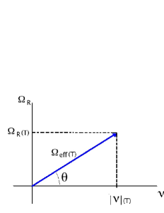
Figure 1: Effective Rabi frequency $\Omega_{\rm eff}=\sqrt{\Omega_{R}^{2}+|\nu|^{2}}$ as parametrized by equations (33) and (34). While $\Omega_{\rm eff}$ is strongly temperature dependent, as shown in Eq. (74), the angle given by $\tan\theta=\Omega_{R}/|\nu|$ is not affected by thermal fluctuations.

Moreover, the condensate fraction of both species depends on the ratio $\Omega_{R}/|\nu|$. It is instructive to parametrize $\Omega_{R}$ and $|\nu|$ in the following way (as shown in Fig. (1)),

$$\Omega_{R} = \Omega_{\rm eff}\sin\theta,$$ (33)

$$|\nu| = \Omega_{\rm eff}\cos\theta,$$ (34)

with $0\leq\theta\leq\pi/2$. In terms of this parametrization, the ratio between the condensate densities takes the form

$$\frac{|\phi_{0}|^{2}}{|\psi_{0}|^{2}}=\sec^{2}\theta\left(1-\sin\theta\right)^{2},$$ (35)

which does not depend on $\Omega_{\rm eff}$ but only on $\tan\theta=\Omega_{R}/|\nu|$. We depict this function in Fig. (2).

Figure 2: $|\phi_{0}|^{2}/|\psi_{0}|^{2}$ given by Eq. (35) as a function of $\theta$, where $\tan\theta=\Omega_{R}/|\nu|$.

For $\theta\rightarrow 0$ or $\Omega_{R}\rightarrow 0$ with $|\nu|\neq 0$, both condensates have essentially the same fraction. On the other hand, for $\theta\rightarrow\pi/2$ or $|\nu|\rightarrow 0$ with $\Omega_{R}\neq 0$, only one of the fields condensates. We will show in the next section that, while $\Omega_{\rm eff}$ is renormalized by temperature, the present result is temperature independent.

5 Effect of Fluctuations

To study thermal as well as quantum fluctuations, we start by considering the following Euclidean ($\tau=it$) finite temperature field theory:

$$S_{\mathrm{E}}(\beta)=\int_{0}^{\beta}d\tau\int d^{3}x\left[\varphi_{1}^{\ast}\left(\partial_{\tau}-\frac{\nabla^{2}}{2m}-\mu_{+}\right)\varphi_{1}\right.$$ (36)

$$+ \left.\varphi_{2}^{\ast}\left(\partial_{\tau}-\frac{\nabla^{2}}{2m}-\mu_{-}\right)\varphi_{2}+\frac{g}{2}\left(\varphi_{1}^{\ast}\varphi_{1}+\varphi_{2}^{\ast}\varphi_{2}\right)^{2}\right]$$

with $\beta=1/T$. The partition function reads

$$Z(\beta,\vec{J}) = \int\mathcal{D}\varphi_{1}\mathcal{D}\varphi_{1}^{\ast}\mathcal{D}\varphi_{2}\mathcal{D}\varphi_{2}^{\ast}\;e^{-S_{\mathrm{E}}+\int d^{3}xd\tau\vec{J}\cdot\vec{\varphi}}$$ (37)

$$= e^{-\beta VW[\beta,J]},$$

where we have introduced a source $\vec{J}$ in order to compute field correlation functions. The functional integration measure implicitly contains the cyclic bosonic boundary condition in Euclidean time, $\varphi_{1,2}(0,x)=\varphi_{1,2}(\beta,x)$. $W[\beta,\vec{J}]=-\frac{1}{\beta V}\ln Z$ is the Helmholtz free energy density.

The main purpose of this section is to compute $W[\beta,J]$ in mean-field approximation plus Gaussian fluctuations. We expect that, at least in a certain temperature range, fluctuations will not change the general mean-field structure. With this in mind, in order to compute $W[\beta,J]$ we replace in Eq. (37) the following decomposition

$$\varphi_{1}(x,\tau) = \varphi_{1}^{0}+\tilde{\varphi}_{1}(x,\tau)$$ (38)

$$\varphi_{2}(x,\tau) = \tilde{\varphi}_{2}(x,\tau)$$ (39)

in which $\int d^{3}x\;\tilde{\varphi}_{1,2}=0$ and $\varphi_{1}^{0}(J)$ is a solution of the mean field equations,

$$\left.\frac{\delta S_{E}}{\delta\varphi_{1}}\right|_{\varphi_{1}=\varphi_{1}^{0},\varphi_{2}=0} = J\;,$$ (40)

$$\left.\frac{\delta S_{E}}{\delta\varphi_{2}}\right|_{\varphi_{1}=\varphi_{1}^{0},\varphi_{2}=0} = 0\;,$$ (41)

where we have chosen a constant source $\vec{J}$, pointing in the $\varphi_{1}$ direction.

Retaining up to second-order terms in the fluctuations we obtain

$$Z(\beta)=e^{-\beta VU_{0}(\varphi_{1}^{0})}\int\left[\mathcal{D}\tilde{\varphi}\right]\;e^{-\int d\tau d^{3}x\sum_{ij}\tilde{\varphi}_{i}^{\ast}S_{ij}^{(2)}\tilde{\varphi}_{j}}\;,$$ (42)

where

$$U_{0}=-\mu_{+}|\varphi_{1}^{0}|^{2}+\frac{g}{2}|\varphi_{1}^{0}|^{4}\;\;.$$ (43)

The integration measure is

$$[\mathcal{D}\tilde{\varphi}]=\mathcal{D}\tilde{\varphi}_{1}\mathcal{D}\tilde{\varphi}_{1}^{\ast}\mathcal{D}\tilde{\varphi}_{2}\mathcal{D}\tilde{\varphi}_{2}^{\ast}$$ (44)

and the quadratic kernel,

$$S_{ij}^{(2)}=\left.\frac{\delta^{2}S_{\mathrm{E}}}{\delta\varphi_{j}^{\ast}\delta\varphi_{i}}\right|_{\varphi_{1}=\varphi_{1}^{0},\varphi_{2}=0}\;\;,$$ (45)

with $i,j=1,2$.

Integrating out quadratic fluctuations, we find an expression for the free energy density,

$$W[J,\beta]=U_{0}+\Delta W$$ (46)

with

$$\Delta W[J,\beta]=\frac{1}{2}\ln\det\hat{S}^{(2)}=\frac{1}{2}{\rm Tr}\ln\hat{S}^{(2)}\;.$$ (47)

The matrix $\hat{S}^{(2)}$ in the {Re$(\tilde{\varphi}_{1})$, Im$(\tilde{\varphi}_{1})$, Re$(\tilde{\varphi}_{2})$, Im$(\tilde{\varphi}_{2})$} basis decouples into two independent $2\times 2$ blocks,

$$\hat{S}^{(2)}=\left(\begin{array}[]{cc}\hat{S}_{a}^{(2)}&0\\ 0&\hat{S}_{b}^{(2)}\end{array}\right),$$ (48)

with

$$\hat{S}_{a}^{(2)}=\left(\begin{array}[]{cc}-\frac{\nabla^{2}}{2m}-\mu_{+}+3g|\varphi_{1}^{0}|^{2}&i\partial_{\tau}\\ -i\partial_{\tau}&-\frac{\nabla^{2}}{2m}-\mu_{+}+g|\varphi_{1}^{0}|^{2}\end{array}\right)$$ (49)

and

$$\hat{S}_{b}^{(2)}=\left(\begin{array}[]{cc}-\frac{\nabla^{2}}{2m}-\mu_{-}+g|\varphi_{1}^{0}|^{2}&i\partial_{\tau}\\ -i\partial_{\tau}&-\frac{\nabla^{2}}{2m}-\mu_{-}+g|\varphi_{1}^{0}|^{2}\end{array}\right).$$ (50)

It is not difficult to compute the trace in Fourier space, obtaining

$$\Delta W=\frac{1}{2\beta}\sum_{n=-\infty}^{+\infty}\int\frac{d^{3}q}{(2\pi)^{3}}\ln\left\{\left(\omega_{n}^{2}+E_{1}^{2}\right)\left(\omega_{n}^{2}+E_{2}^{2}\right)\right\},$$ (51)

where $\omega_{n}=2\pi n/\beta$ are the Matsubara frequencies,

$$E_{1}=\sqrt{\left(\frac{q^{2}}{2m}-\mu_{+}+3g|\varphi_{1}^{0}|^{2}\right)\left(\frac{q^{2}}{2m}-\mu_{+}+g|\varphi_{1}^{0}|^{2}\right)}$$ (52)

and

$$E_{2}=\frac{q^{2}}{2m}-\mu_{-}+g|\varphi_{1}^{0}|^{2}\;.$$ (53)

Summing up the Matsubara frequencies, using

$$\frac{1}{\beta}\sum_{n}\ln(\omega_{n}^{2}+E_{i}^{2})=E_{i}+\frac{2}{\beta}\ln\left(1-e^{-\beta E_{i}}\right),$$ (54)

we obtain

$$\Delta W=\frac{1}{2}\int\frac{d^{3}q}{(2\pi)^{3}}\sum_{i}\left\{E_{i}+\frac{2}{\beta}\ln\left(1-e^{-\beta E_{i}}\right)\right\}.$$ (55)

It is interesting to note that, if we substitute the mean-field value for $\varphi_{1}^{0}$, given by Eq. (29), into Eqs. (52) and (53), we immediately obtain

$$\tilde{E}_{1}=\sqrt{\left(\frac{q^{2}}{2m}\right)\left(\frac{q^{2}}{2m}+2g|\varphi_{1}^{0}|^{2}\right)}$$ (56)

and

$$\tilde{E}_{2}=\frac{q^{2}}{2m}+2\Omega_{\rm eff}\;.$$ (57)

Equations. (56) and (57) are the usual energy excitations computed in the Bogoliubov approximation. Note that $\lim_{q\rightarrow 0}\tilde{E}_{1}=0$, corresponding with the Goldstone mode associated with the spontaneous breakdown of the $U_{\varphi_{1}}(1)$ symmetry, while Eq. (57) is a gapped mode corresponding to non-condensate fluctuations.

It is useful to express the free energy $W(\beta,J)$ in terms of the order parameter:

$$\bar{\varphi}=\delta W/\delta J=\varphi_{1}^{0}+\frac{1}{2}\mathrm{Tr}\left[\frac{1}{\hat{S}^{(2)}}\frac{\delta\hat{S}^{(2)}}{\delta\varphi_{1}^{0}}\frac{\delta\varphi_{1}^{0}}{\delta J}\right]\;.$$ (58)

At mean-field level, the order parameter is exactly the mean-field solution $\varphi_{1}^{0}$. However, when fluctuations are taken into account, the result given by Eq. (58) is more involved.

We define the Gibbs free energy as a functional of the order parameter $\bar{\varphi}$ by making a Legendre transformation

$$\Gamma[\beta,\bar{\varphi}]=\bar{\varphi}J-W\;,$$ (59)

where $\delta\Gamma/\delta\bar{\varphi}=J$. In Eq. (59), $J$ is a function of the order parameter $\bar{\varphi}$ obtained by inverting Eq. (58). To leading order in the fluctuations the result is

$$\Gamma[\beta,\bar{\varphi}] = \mu_{+}|\bar{\varphi}|^{2}-\frac{g}{2}|\bar{\varphi}|^{4}$$ (60)

$$- \frac{1}{2}\int\frac{d^{3}q}{(2\pi)^{3}}\sum_{i}\left\{E_{i}+\frac{2}{\beta}\ln\left(1-e^{-\beta E_{i}}\right)\right\}.$$

This is the Gibbs free energy computed at mean field plus Gaussian fluctuations or, in the language of quantum field theory, the finite temperature one-loop effective action.

The actual condensate amplitude $\bar{\varphi}_{m}$ is computed by minimizing the free energy,

$$\left.\frac{\partial\Gamma[\beta,\bar{\varphi}]}{\partial\bar{\varphi}}\right|_{\bar{\varphi}=\bar{\varphi}_{m}}=0.$$ (61)

By analogy with the mean field solution $|\varphi_{1}^{0}|^{2}=\mu_{+}/g$ we can define an effective chemical potential in the following way,

$$|\bar{\varphi}_{m}|^{2}(T)=\frac{1}{g}\;\bar{\mu}_{+}(T),$$ (62)

where now $\bar{\mu}_{+}(T)$ is the effective chemical potential for the $\varphi_{1}$ component, renormalized by quantum as well as thermal fluctuations. Using Eqs. (60) and (61), we obtain an expression for $\bar{\mu}_{+}(T)$ in terms of the original bare $\mu_{+}$,

$$\bar{\mu}_{+}=\mu_{+}-\frac{1}{2}\int\frac{d^{3}q}{(2\pi)^{3}}\times$$ (63)

$$\times \left\{\frac{(2\frac{q^{2}}{2m}+\bar{\mu}_{+})(1+2n(E_{1}))}{\sqrt{\left(\frac{q^{2}}{2m}\right)\left(\frac{q^{2}}{2m}+2\bar{\mu}_{+}\right)}}+1+2n(E_{2})\right\},$$

where $n(E_{i})$ is the usual Bose distribution

$$n(E_{i})=\frac{1}{e^{\beta E_{i}}-1}$$ (64)

with $i=1,2$.

The total particle density of each species can be computed as

$$\rho_{\varphi_{1}} = \left.\frac{\partial\Gamma}{\partial\mu_{+}}\right|_{\bar{\varphi}_{m}}=\frac{\mu_{+}}{g}-\frac{1}{2}\int\frac{d^{3}q}{(2\pi)^{3}}\frac{q^{2}/2m}{E_{1}}(1+2n(E_{1}))$$ (65)

$$\mbox{\hskip 51.21504pt}-\frac{1}{2}\int\frac{d^{3}q}{(2\pi)^{3}}(1+2n(E_{2}))\;,$$

$$\rho_{\varphi_{2}} = \left.\frac{\partial\Gamma}{\partial\mu_{-}}\right|_{\bar{\varphi}_{m}}=\frac{1}{2}\int\frac{d^{3}q}{(2\pi)^{3}}(1+2n(E_{2}))\;.$$ (66)

Using the relation between $\mu_{+}$ and $\bar{\mu}_{+}$ given by Eq. (63), we finally get

$$\rho_{\varphi_{1}} = \frac{\bar{\mu}_{+}}{g}+\frac{1}{2}\int\frac{d^{3}q}{(2\pi)^{3}}\frac{\frac{q^{2}}{2m}+\bar{\mu}_{+}}{E_{+}}\coth(\beta E_{+}/2),$$ (67)

$$\rho_{\varphi_{2}} = \frac{1}{2}\int\frac{d^{3}q}{(2\pi)^{3}}\coth(\beta E_{-}/2),$$ (68)

with

$$E_{+} = \sqrt{\left(\frac{q^{2}}{2m}\right)\left(\frac{q^{2}}{2m}+2\bar{\mu}_{+}(T)\right)},$$ (69)

$$E_{-} = \frac{q^{2}}{2m}+2\bar{\Omega}_{\rm eff}(T)\;,$$ (70)

where we have defined the renormalized effective Rabi frequency $\bar{\Omega}_{\rm eff}(T)=(\bar{\mu}_{+}-\bar{\mu}_{-})/2$ as a difference between the renormalized chemical potentials, in analogy with the bare effective Rabi frequency $\Omega_{\rm eff}=(\mu_{+}-\mu_{-})/2$. Notice that, while Eq. (67) completely determines $\bar{\mu}_{+}$, Eq. (68) is the definition of the renormalized chemical potential $\bar{\mu}_{-}$, through the expression for the excitation energy $E_{-}$ (Eq. (70)). In terms of these variables, Eqs. (67) and (68) are coupled equations. However, it is more convenient to work with $\bar{\mu}_{+}$ and $\bar{\Omega}_{\rm eff}$ as independent variables, in such a way that Eqs. (67) and (68) are now decoupled equations. In terms of these variables, all other chemical potentials are linear combinations of the former, such as, $\bar{\mu}_{-}=\bar{\mu}_{+}-2\bar{\Omega}_{\rm eff}$ and $\bar{\mu}=\bar{\mu}_{+}-\bar{\Omega}_{\rm eff}$.

Expressions (67) and (68) have the usual ultraviolet divergences of a field theory at $T=0$. As is well known, temperature fluctuations are always convergent. The usual way to deal with this divergence is to regularize the integral and then renormalize the bare constants $\mu_{+}$, $\mu_{-}$ and $g$, in order to obtain finite results. A convenient procedure, in the non-relativistic scalar case, is the cut-off technique. If we simply limit the momentum integrals using an ultraviolet cut-off, $0\leq|\vec{q}|\leq\Lambda$, the results are obviously $\Lambda$-dependent. However, if we begin the calculations with renormalized constants, $\mu_{\pm}^{R}=\mu_{\pm}+\delta\mu_{\pm}(\Lambda)$, we can adjust $\delta\mu_{\pm}(\Lambda)$ to make the result independent of $\Lambda$. At the end, we can safely take the limit $\Lambda\rightarrow\infty$. After this procedure, the renormalized expressions read

$$\rho_{\varphi_{1}} = \frac{\bar{\mu}_{+}}{g}+\frac{(m\bar{\mu}_{+})^{3/2}}{3\pi^{2}}+\int\frac{d^{3}q}{(2\pi)^{3}}\frac{\frac{q^{2}}{2m}+\bar{\mu}_{+}}{E_{+}(e^{\beta E_{+}}-1)},$$ (71)

$$\rho_{\varphi_{2}} = \int\frac{d^{3}q}{(2\pi)^{3}}\frac{1}{e^{\beta E_{-}}-1}\ .$$ (72)

Equation (71) implicitly defines the condensate density $\bar{\varphi}_{m}(T)$ or, equivalently, the effective chemical potential $\bar{\mu}_{+}(T)$, given by Eq. (62). This equation coincides with that derived from a one-loop effective potential of a single self-interacting field [27]. Moreover, eq. (72) determines the effective Rabi frequency, $\bar{\Omega}_{\mathrm{eff}}(T)$ through the expression for $E_{-}$, Eq. (70). In Eqs. (71) and (72), $\rho_{\varphi_{1}}$ and $\rho_{\varphi_{2}}$ are two independent constants, since the particle number of each species is conserved independently, due to the symmetry $U_{\varphi_{1}}(1)\otimes U_{\varphi_{2}}(1)$. The critical temperature, $T_{c}$, is easily computed by fixing $\bar{\mu}_{+}(T_{c})=0$ in Eq. (71), obtaining the usual expression for an ideal gas,

$$T_{c}=\frac{2\pi}{m\zeta(3/2)^{2/3}}\rho_{\varphi_{1}}^{2/3},$$ (73)

with $\zeta(3/2)\sim 2.612$. We expect corrections of $T_{c}$ only at a two-loop approximation [38, 39]. Since $E_{-}$ are gapped energy excitations, the integral in Eq. (72) can be safely done in the classical limit. Solving for $\bar{\Omega}_{\rm eff}(T)$ we obtain,

$$\bar{\Omega}_{\mathrm{eff}}(T)=\frac{T}{2}\ln\left[\left(\frac{\rho_{\varphi_{1}}}{\rho_{\varphi_{2}}}\right)\left(\frac{T}{T_{c}}\right)^{3/2}\right]\;.$$ (74)

Note that there is a minimum temperature for which $\bar{\Omega}_{\rm eff}(T_{r})=0$, given by $T_{r}=(\rho_{\varphi_{2}}/\rho_{\varphi_{1}})^{2/3}T_{c}$. At this temperature, the $O(2)$ symmetry is restored. This reentrance transition makes the excitation energy $E_{-}$ (Eq. (70)) gapless, producing an instability of the mean-field solution. Then, at this temperature, the chosen mean-field solution is unstable under Gaussian fluctuations. In order to have the condensate structure given by Eqs. (30) and (31), we need to fix $\rho_{\varphi_{2}}/\rho_{\varphi_{1}}<1$ and $T_{r}<T<T_{c}$. In the next section, we numerically compute the condensate fractions as functions of temperature for different values of the parameters.

6 Numerical results

To compute the condensate density profile we rewrite Eq. (71) in dimensionless form. For this, we define the condensate fraction $\rho_{c}=\bar{\mu}_{+}/(g\rho_{\varphi_{1}})$. The dimensionless temperature is defined as $\bar{T}=T/T_{c}$ and we introduce the diluteness parameter $n_{\varphi_{1}}=\rho_{\varphi_{1}}a^{3}$, where $a$ is the s-wave scattering length. Using these definitions, we can write Eq. (71) in the following form:

$$1 = \rho_{c}+\frac{8}{3\pi^{1/2}}n_{\varphi_{1}}^{1/2}\rho_{c}^{3/2}$$ (75)

$$+ \frac{4}{\pi^{1/2}\zeta(3/2)}\bar{T}^{3/2}\int_{0}^{\infty}dyy\frac{y^{2}+2\zeta(3/2)^{2/3}n_{\varphi_{1}}^{1/3}\rho_{c}\bar{T}^{-1}}{\sqrt{y^{2}+4\zeta(3/2)^{2/3}n_{\varphi_{1}}^{1/3}\rho_{c}\bar{T}^{-1}}}$$

$$\times \left(e^{y\sqrt{y^{2}+4\zeta(3/2)^{2/3}n_{\varphi_{1}}^{1/3}\rho_{c}\bar{T}^{-1}}}-1\right)^{-1}\;\;.$$

It is simple to check that the limit $n_{\varphi_{1}}\rightarrow 0$ leads to the ideal gas result $\rho_{c}=1-\bar{T}^{3/2}$. The second term of the r.h.s. of eq. (75) gives the quantum depletion of the condensate, while the third term represents the temperature dependence. Numerically solving Eq. (75), we can obtain the condensate fraction $\rho_{c}(\bar{T})$ for different values of the diluteness parameter $n_{\varphi_{1}}$. From this result, it is simple to compute the condensate fractions for the original fields $\phi$ and $\psi$, using Eqs. (30) and (31).

We define the condensate fractions for the fields $\phi$ and $\psi$ as $\rho^{c}_{\phi}=|\phi_{0}|^{2}/(\rho_{\varphi_{1}}+\rho_{\varphi_{2}})$ and $\rho^{c}_{\psi}=|\psi_{0}|^{2}/(\rho_{\varphi_{1}}+\rho_{\varphi_{2}})$, where we chose the total particle density $\rho_{\phi}+\rho_{\psi}=\rho_{\varphi_{1}}+\rho_{\varphi_{2}}$ to normalize the fractions. Then, we use Eqs. (30) and (31) to relate $\rho^{c}_{\phi}$ and $\rho^{c}_{\psi}$ with $\rho_{c}$, given by Eq. (75).

There are two interesting regimes to focus on. For $|\nu|/\Omega_{R}\ll 1$, the condensate fractions become

$$\rho_{\phi}^{c} \sim \left(1-\frac{\rho_{\varphi_{2}}}{\rho_{\varphi_{1}}}\right)\left(\frac{|\nu|}{2\Omega_{R}}\right)^{2}\rho_{c}\;,$$ (76)

$$\rho_{\psi}^{c} \sim \left(1-\frac{\rho_{\varphi_{2}}}{\rho_{\varphi_{1}}}\right)\rho_{c}\;.$$ (77)

The first factor compensates the normalizations of $\rho_{\phi,\psi}^{c}$ and $\rho_{c}$. To obtain it, we have considered $\rho_{\varphi_{2}}/\rho_{\varphi_{1}}<1$ and we have dropped terms proportional to $(\rho_{\varphi_{2}}/\rho_{\varphi_{1}})^{2}$. The condensate fraction is determined by the factor $(|\nu|/2\Omega_{R})^{2}$ and the next corrections to eqs. (76) and (77) are proportional to $(|\nu|/2\Omega_{R})^{4}$. In Fig. (3) we show the typical profile of both condensates, where we have fixed $n_{\varphi_{1}}=10^{-5}$, $\rho_{\varphi_{2}}/\rho_{\varphi_{1}}=10^{-1}$ and $|\nu|/2\Omega_{R}=0.24$. Note that $\rho_{\phi}^{c}$ is strongly suppressed by the factor $\nu/\Omega_{R}$ and tends to disappear in the limit $|\nu|\rightarrow 0$. An interesting observation is that the factor $|\nu|/\Omega_{R}$ is not corrected by temperature fluctuations. This is a direct consequence of the $O(2)$ symmetry of the two-body interaction.

Figure 3: Condensate fractions as functions of the dimensionless temperature $\bar{T}$ in the limit $|\nu|/\Omega_{R}<1$. The solid line represents $\rho_{\psi}^{c}$, given by eq. (77), while the dashed line is $\rho_{\phi}^{c}$, given by eq. (76). We have fixed $n_{\varphi_{1}}=10^{-5}$, $\rho_{\varphi_{2}}/\rho_{\varphi_{1}}=10^{-1}$ and $|\nu|/2\Omega_{R}=0.24$.

In the opposite regime $\Omega_{R}/|\nu|\ll 1$, the condensate densities of both species are essentially equal, with small corrections, given by

$$\rho^{c}_{\phi_{0}} \sim \frac{1}{2}\left(1-\frac{\rho_{\varphi_{2}}}{\rho_{\varphi_{1}}}\right)\left(1-\frac{\Omega_{R}}{|\nu|}\right)\rho_{c}\;,$$ (78)

$$\rho^{c}_{\psi_{0}} \sim \frac{1}{2}\left(1-\frac{\rho_{\varphi_{2}}}{\rho_{\varphi_{1}}}\right)\left(1+\frac{\Omega_{R}}{|\nu|}\right)\rho_{c}\;,$$ (79)

where we have discarded corrections of order $(\Omega_{R}/|\nu|)^{2}$. We show these curves in Fig. (4) for $n_{\varphi_{1}}=10^{-5}$, $\rho_{\varphi_{2}}/\rho_{\varphi_{1}}=10^{-1}$ and $\Omega_{R}/|\nu|=0.02$.

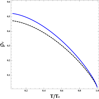
Figure 4: Condensate fractions as functions of the dimensionless temperature $\bar{T}$ in the limit $\Omega_{R}/|\nu|<1$. The solid line represents $\rho_{\psi}^{c}$, given by eq. (79), while the dashed line is $\rho_{\phi}^{c}$, given by eq. (78). We have fixed $n_{\varphi_{1}}=10^{-5}$, $\rho_{\varphi_{2}}/\rho_{\varphi_{1}}=10^{-1}$ and $\Omega_{R}/|\nu|=0.02$.

7 Discussion

We have addressed the problem of equilibrium properties of a uniform mixture of two bosonic fields in the presence of Josephson-type interactions. We have considered a quantum field theory built by two non-relativistic complex bosonic fields with general two-body local interactions. We have focused on a particular symmetry point, in which, in addition to the $U(1)\otimes U(1)$ phase symmetry, there is an emergent $O(2)$ symmetry, related with rotations in the isospin space $(\phi,\psi)$. We have minimally perturbed this model by considering the effect of Josephson couplings that unbalance the species population by transferring charge from one species to the other. These interactions are parametrized by the Rabi frequency $\Omega_{R}$ and the detuning $\nu$. By making a rotation in the isospin space, $(\phi,\psi)\rightarrow(\varphi_{1},\varphi_{2})$, we have shown that there is a special direction for which the $U(1)\otimes U(1)$ phase symmetry is recovered and only one of the bosonic species (say $\varphi_{1}$) could eventually condensate in this framework. In this basis, the density of each bosonic species $\rho_{\varphi_{1}}$ and $\rho_{\varphi_{2}}$ is conserved independently. Of course, the $O(2)$ symmetry is still broken, provided the difference between chemical potentials $\Delta\mu=\mu_{+}-\mu_{-}=2\Omega_{\mathrm{eff}}\neq 0$.

In the $(\varphi_{1},\varphi_{2})$ basis, it is simpler to compute fluctuations. Specifically, we have computed finite temperature one-loop effective action (the Gibbs free energy) as a function of the order parameter and the temperature. In this way, by minimizing the free energy, we have obtained the condensate fraction. Since the total density of each species is conserved in this basis, the constant values of $\rho_{\varphi_{1}}$ and $\rho_{\varphi_{2}}$ completely determine the two chemical potentials $\bar{\mu}_{+}$ and $\bar{\mu}_{-}$. Alternatively, there is an interesting decoupling if we work in terms of the parameters $\bar{\mu}_{+}$ and $\bar{\Omega}_{\rm eff}$. While the density $\rho_{\varphi_{1}}$ fixes the value of $\bar{\mu}_{+}(T)$, the value of $\rho_{\varphi_{2}}$ determines the value of $\bar{\Omega}_{\rm eff}(T)$. In this way, we can explicitly compute two limiting temperatures given by $\bar{\mu}_{+}(T_{c})=0$ and $\Omega_{\rm eff}(T_{r})=0$. $T_{c}$ is the critical temperature for the Bose-Einstein condensation and $T_{r}$ is a reentrance temperature where the $O(2)$ symmetry is recovered. Below this temperature, the mean-field solution is unstable under thermal fluctuations. Thus, our results are only valid for $T_{r}<T<T_{c}$. To compute the condensate fractions below $T_{r}$, it is necessary to assume that both species in the rotated frame ($\varphi_{1},\varphi_{2}$) could condensate, making the computation of fluctuations more involved.

To obtain the condensate profiles of the original fields, we rotated back to the original basis $(\phi,\psi)$. This rotation only depends on the ratio $\Omega_{R}/|\nu|$. It is interesting to note that, due to the $O(2)$ symmetry of the two-body interaction, fluctuations only renormalize the effective Rabi frequency $\Omega_{\mathrm{eff}}=\sqrt{\Omega_{R}^{2}+|\nu|^{2}}$, while the ratio $\Omega_{R}/|\nu|$ remains unaffected. Thus, the isospin rotation coefficients are temperature independent.

In figures (3) and (4) we show the condensate profiles of the $\psi$ and $\phi$ species as functions of the temperature for different values of the parameter $\Omega_{R}/|\nu|$. We have shown that, for a temperature interval $T_{r}<T<T_{c}$, both bosonic species condensate and the relatives phases are locked by the laser phase $\alpha$. We also have shown that the ratio between the condensates essentially depends on the temperature-independent parameter $\Omega_{R}/|\nu|$. We clearly see that, for $|\nu|/\Omega_{R}\rightarrow 0$, only one condensate survives, while in the opposite limit $\Omega_{R}/|\nu|\rightarrow 0$, both condensates are essentially equal, with small corrections of order $\Omega_{R}/|\nu|$.

The results presented in this paper are valid, provided the two-body interaction is invariant under isospin rotations. Consider, for instance, a small deviation from the $O(2)$ model, $g_{\phi}=g_{\psi}=g$, but $g_{\psi\phi}=g+\Delta g$. Upon rotation to the $(\varphi_{1},\varphi_{2})$ basis, a term proportional to $\Delta g(\varphi_{1}^{\ast}\varphi_{1}^{\ast}\varphi_{2}\varphi_{2})$ will be generated. Thus, even though we have ignored this type of terms in the original model, they will be generated in a more general two-body interaction case. Thus, for $\Delta g\neq 0$, there is no isospin direction in which the $U(1)\otimes U(1)$ symmetry is recovered. This fact makes the study of quantum and thermal fluctuations more involved. We hope to report on this issue shortly.

Appendix A Rabi frequency and detuning

Although Rabi frequency and detuning are very well known concepts in atomic physics and Raman spectroscopy, we would like to sketch in this appendix a brief summary relevant for the definition of our model.

The general context is the study of transition probabilities between hyperfine atomic states induced by an electromagnetic interaction. Just to keep matters simple, consider, for instance, a two-level quantum system interacting with a classical electromagnetic field. The eigenstates of the free Hamiltonian are characterized by the two-dimensional orthogonal basis $\{|1\rangle,|2\rangle\}$, in such a way that the energies $E_{1},E_{2}$ are the eingenvalues of the free Hamiltonian $H_{0}$,

$$H_{0}|1\rangle = E_{1}|1\rangle,$$ (80)

$$H_{0}|2\rangle = E_{2}|2\rangle$$ (81)

and $\langle 1|1\rangle=\langle 2|2\rangle=1$, $\langle 1|2\rangle=\langle 2|1\rangle=0$. In this way, a general time dependent state can be written as

$$|\psi(t)\rangle=C_{1}(t)|1\rangle+C_{2}(t)|2\rangle$$ (82)

with $|C_{1}|^{2}+|C_{2}|^{2}=1$. Defining the spinor $\psi(t)=\{C_{1}(t),C_{2}(t)\}$, the Shrödinger equation reads

$$i\hbar\frac{d\psi}{dt}=\hat{H}\psi\ ,$$ (83)

with $\hat{H}=\hat{H}_{0}+\hat{H}_{\rm int}$ and

$$\hat{H}_{0}=\left(\begin{array}[]{cc}E_{1}&0\\ 0&E_{2}\end{array}\right).$$ (84)

To built the interaction Hamiltonian we consider that the electromagnetic field induces a dipole moment between the states $|1\rangle$ and $|2\rangle$ and the electric field couples with this dipole moment in such a way that

$$\hat{H}_{\rm int}=\left(\begin{array}[]{cc}0&\hbar\Omega_{R}\cos(\omega t+\alpha)\\ \hbar\Omega_{R}\cos(\omega t+\alpha)&0\end{array}\right),$$ (85)

where $\hbar\Omega_{R}$ is the dipole interaction energy, $\omega$ and $\alpha$ are the frequency and phase of the electromagnetic field respectively. The coupling $\Omega_{R}$ is usually called the Rabi frequency, while the frequency $\omega=(E_{1}-E_{2})/\hbar+|\nu|$, where $|\nu|$ is the detuning of the frequency related with the resonance frequency $\omega_{0}=(E_{1}-E_{2})/\hbar$. If we consider that at the initial time $t=0$ the system is in the ground state $|1\rangle$, we can easily solve the equation (83) with the initial conditions $C_{1}(0)=1,C_{2}(0)=0$, finding

$$|C_{1}(t)|^{2}=\left(\frac{|\nu|}{\Omega_{\rm eff}}\right)^{2}\left[1+\left(\frac{\Omega_{R}}{|\nu|}\right)^{2}\cos^{2}\left(\frac{\Omega_{\rm eff}t}{2}\right)\right],$$ (86)

where ${\Omega_{\rm eff}}=\sqrt{\Omega_{R}^{2}+|\nu|^{2}}$ is called the effective Rabi frequency and $|C_{2}(t)|^{2}=1-|C_{1}(t)|^{2}$.

Thus, the dynamical behavior of the two-level system is driven by two parameters, the Rabi frequency $\Omega_{R}$, which measures the coupling strength of the dipole with the electromagnetic field, and the detuning $|\nu|$, which measures the distance between the frequency of the applied field and the resonance frequency $\omega_{0}=(E_{1}-E_{2})/\hbar$. Notice that the time dependency is completely given by the effective Rabi frequency $\Omega_{\rm eff}$, while the ratio $\Omega_{R}/|\nu|$ controls the amplitude of the probability density.

Consider the system near the resonance (very small detuning) and in a weak coupling regime (small Rabi frequency). Then, the usual rotating wave approximation can be performed. It consists in writing the Hamiltonian in the interaction picture discarding rapidly fluctuating terms (terms that oscillates with $2\omega$). In this approximation, the Hamiltonian takes the simpler form

$$\hat{H}=\left(\begin{array}[]{cc}|\nu|&\Omega_{R}e^{i\alpha}\\ \Omega_{R}e^{-i\alpha}&-|\nu|\end{array}\right)$$ (87)

(where we have set $\hbar=1$). This form of the one-particle Hamiltonian was used in Ref. [34] to describe effective spin-orbit interactions in two bosonic species systems.

Equivalently, we can make another unitary transformation of the form

$$\hat{H}^{\prime}=U^{\dagger}\hat{H}U\ ,$$ (88)

with

$$U=\frac{i}{\sqrt{2}}\left(\begin{array}[]{cc}e^{i\alpha}&1\\ 1&-e^{-i\alpha}\end{array}\right)\;$$ (89)

and $U^{\dagger}U=I$, obtaining

$$\hat{H}^{\prime}=\left(\begin{array}[]{cc}\Omega_{R}&|\nu|e^{-i\alpha}\\ |\nu|e^{i\alpha}&-\Omega_{R}\end{array}\right)\;.$$ (90)

This form of the one-body Hamiltonian was considered in Ref. [33] to study spin-orbit couplings and it is the form we have adopted to build our model.

The model discussed in our paper is evidently more complex than the simple model described in this appendix, since it is composed by two interacting fields. While the condensates could be considered in some approximation as a two-level system, fluctuations out of the condensate strongly renormalized the bare parameters $\Omega_{R}$ and $\nu$. We showed that the effective Rabi frequency $\Omega_{\rm eff}$ is strongly renormalized by temperature, while the ratio $\Omega_{R}/|\nu|$ is unaffected by thermal fluctuations.

References

- [1] Sebastian Will, “From Atom Optics to Quantum Simulation: Interacting Bosons and Fermions in Three-Dimensional Optical Lattice Potentials” , Springer-Verlag Berlin, Heidelberg (2013).
- [2] P. Soltan-Panahi, J. Struck, P. Hauke, A. Bick, W. Plenkers, G. Meineke, C. Becker, P. Windpassinger, M. Lewenstein, and K. Sengstock, Nature Physics 7, 434 (2011).
- [3] M. R. Andrews, C. G. Townsend, H. J. Miesner, D. S. Durfee, D. M. Kurn, and W. Ketterle, Science 175, 637 (1997).
- [4] Bryce Gadway, Daniel Pertot, René Reimann, and Dominik Schneble, Phys. Rev. Lett. 105, 045303 (2010).
- [5] M. Iskin, C. A. R. Sa de Melo, Phys. Rev. Lett. 97, 100404 (2006); Phys. Rev. A 83, 045602 (2011).
- [6] C. J. Myatt, E. A. Burt, R. W. Ghrist, E. A. Cornell and C. E. Wieman, Phys. Rev. Lett. 78, 586 (1997).
- [7] D. S. Hall, M. R. Matthews, J. R. Ensher, C. E. Wieman, and E. A. Cornell, Phys. Rev. Lett. 81, 1539 (1998).
- [8] D. S. Hall, M. R. Matthews, C. E. Wieman, and E. A. Cornell, Phys. Rev. Lett. 81, 1543 (1998).
- [9] Y. J. Lin, K. Jimenez-Garcia, and I.B. Spielman, Nature 471, 83 (2011).
- [10] T. Zibold, E. Nicklas, C. Gross, and M. K. Oberthaler, Phys. Rev. Lett. 105, 204101 (2010).
- [11] A. J. Leggett and F. Sols, Found. Phys. 21, 353 (1991).
- [12] I. Zapata, F. Sols, and A. J. Leggett, Phys. Rev. A 57, R28 (1998).
- [13] B. D. Josephson, Phys. Lett. 1, 251 (1962).
- [14] A. Barone, Quantum Mesoscopic Phemena and Mesoscopic Devices in Microelectronics, NATO Sience Series C: Mathematical and Physical Sciences 559, edited by I. O. Kulik (Kluwer Academic, Dordrecht/Boston), 301 (2000).
- [15] A. J. Leggett, Rev. Mod. Phys. 73, 307 (2001).
- [16] M. Albiez, R. Gati, J. Folling, S. Hunsmann, M. Cristiani, and M. K. Oberthaler, Phys. Rev. Lett. 95, 010402 (2005).
- [17] S. B. Papp, J. M. Pino, and C. E. Wieman, Phys. Rev. Lett. 101, 040402 (2008).
- [18] R. Gati and M. K. Oberthaler, J. Phys. B: At. Mol. Opt. Phys. 40, 10, R61 (2007).
- [19] S. Levy, E. Lahoud, I. Shomroni, and J. Steinhauer, Nature 449, 579 (2007).
- [20] G. Mazzarella, B. Malomed, L. Salasnich, M. Salerno, and F. Toigo, J. Phys. B: At. Mol. Opt. Phys. 44, 035301(2011).
- [21] A. Smerzi, S. Fantoni, S. Giovanazzi, and S. R. Shenoy, Phys. Rev. Lett. 79, 4950 (1997).
- [22] S. Raghavan, A. Smerzi, S.Fantoni, and S. R. Shenoy, Phys. Rev. A 59, 620 (1999).
- [23] M. Salerno, Laser Physics 4, 620 (2005).
- [24] B. Julia-Diaz, M. Guilleumas, M. Lewenstein, A. Polls, A. Sanpera, Phys. Rev. A 80, 023616 (2009).
- [25] M. Mele-Messeguer, B. Julia-Diaz, M. Guilleumas, A. Polls, A. Sanpera, New Journal of Physics, 13 033012 (2011).
- [26] M. Mele-Messeguer, S. Paganelli, B. Julia-Diaz, A. Sanpera, A. Polls, Phys. Rev. A 86, 053626 (2012).
- [27] M. B. Pinto, R. O. Ramos, and F. F. de Souza Cruz, Phys. Rev. A 74, 033618 (2006).
- [28] M. B. Pinto, Rudnei O. Ramos and Julia E. Parreira, Phys. Rev. D71, 123519 (2005)
- [29] M. B. Pinto and Rudnei O. Ramos, J. Phys. A 39, 6649 (2006); J. Phys. A 39, 6687 (2006).
- [30] Daniel G. Barci, E. S. Fraga, Rudnei O. Ramos, Phys. Rev. Lett. 85, 479 (2000).
- [31] M. Moshe, J. Zinn-Justin, Phys. Rep. 385, 69 (2003).
- [32] Chih-Chun Chien, F. Cooper and E. Timmermans, Phys. Rev. A 86, 023634 (2012).
- [33] M. A. Garcia-March, G. Mazzarella, L. Dell’Anna, B. Juliá-Díaz, L. Salasnich, and A. Polls, Phys. Rev. A 89, 063607 (2014).
- [34] Dan-Wei Zhang,Li-Bin Fu, Z. D. Wang, and Shi-Liang Zhu, Phys. Rev.A 85, 043609 (2012).
- [35] M. R. Matthews et al., Phys. Rev. Lett. 81, 243 (1998).
- [36] K. Rajagopal, F. Wilczek, Nuc. Phys. B399, 395 (1993).
- [37] H. Kleinert, J. Phys. B: At. Mol. Opt. Phys. 46, 175401 (2013).
- [38] F. F. de Souza Cruz, M. B. Pinto, Rudnei O. Ramos and Paulo Sena, Phys. Rev. A65, 053613 (2002).
- [39] F. F. de Souza Cruz, Marcus B. Pinto, Rudnei O. Ramos, Phys.Rev. B64, 014515 (2001).