Abstract

We propose that Bayesian variable selection for linear parametrisations with Gaussian iid likelihoods be based on the spherical symmetry of the diagonalised parameter space. Our r-prior results in closed forms for the evidence for four examples, including the hyper-g prior and the Zellner-Siow prior, which are shown to be special cases. Scenarios of a single variable dispersion parameter and of fixed dispersion are studied, and asymptotic forms comparable to the traditional information criteria are derived. A simulation exercise shows that model comparison based on our r-prior gives good results comparable to or better than current model comparison schemes.

Keywords: canonical linear regression, Zellner-Siow priors, Zellner’s $g$-prior, noninformative priors, AIC, BIC, Model Selection, Gaussian hypergeometric functions

1 Introduction

The overarching problem of variable selection is to choose the best model out of a set of candidate models $\mathcal{M}_{\!\scriptscriptstyle M}$. Given measured data $\mathcal{D}$, the Bayesian solution is to compute the posterior probability for each model with Bayes’ theorem,

$$p(\mathcal{M}_{\!\scriptscriptstyle M}\,|\,\mathcal{D}) =\frac{p(\mathcal{D}\,|\,\mathcal{M}_{\!\scriptscriptstyle M})\,p(\mathcal{M}_{\!\scriptscriptstyle M})}{p(\mathcal{D})}\ =\ \frac{p(\mathcal{D}\,|\,\mathcal{M}_{\!\scriptscriptstyle M})\,p(\mathcal{M}_{\!\scriptscriptstyle M})}{\sum_{\!\scriptscriptstyle M}p(\mathcal{D}\,|\,\mathcal{M}_{\!\scriptscriptstyle M})p(\mathcal{M}_{\!\scriptscriptstyle M})}\,.$$ (1)

As equal priors are usually assigned to the competing models, model comparison becomes a task in finding the marginal likelihood or evidence for each model, i.e. solving the integral over all $K$ model parameters ${\bm{\beta}}_{\!\scriptscriptstyle M}=(\theta_{1},\ldots,\theta_{\!\scriptscriptstyle K})$ of the likelihood $p(\mathcal{D}\,|\,{\bm{\beta}}_{\!\scriptscriptstyle M},\mathcal{M}_{\!\scriptscriptstyle M})$ weighted by the parameter prior $p({\bm{\beta}}_{\!\scriptscriptstyle M}\,|\,\mathcal{M}_{\!\scriptscriptstyle M})$,

$$p(\mathcal{D}\,|\,\mathcal{M}_{\!\scriptscriptstyle M}) =\int p(\mathcal{D}\,|\,{\bm{\beta}}_{\!\scriptscriptstyle M},\mathcal{M}_{\!\scriptscriptstyle M})\,p({\bm{\beta}}_{\!\scriptscriptstyle M}\,|\,\mathcal{M}_{\!\scriptscriptstyle M})\,d{\bm{\beta}}_{\!\scriptscriptstyle M}.$$ (2)

The preferred model will be the one with the largest evidence i.e. with the highest prior-weighted average over all parameters of the likelihood. Where computation of $p(\mathcal{D})$ over the entire model set is impractical or even impossible, this is circumvented by taking ratios of two model probabilities in the form of Bayes Factors, since $p(\mathcal{D})$ cancels and under the equal-model-prior assumption, they become ratios of the respective model evidences,

$$\mathrm{BF}(\mathcal{M}_{\!\scriptscriptstyle M};\mathcal{M}_{{\!\scriptscriptstyle M}^{\prime}}) =\log\frac{p(\mathcal{M}_{\!\scriptscriptstyle M}\,|\,\mathcal{D})}{p(\mathcal{M}_{{\!\scriptscriptstyle M}^{\prime}}\,|\,\mathcal{D})}=\log\frac{p(\mathcal{D}\,|\,\mathcal{M}_{\!\scriptscriptstyle M})}{p(\mathcal{D}\,|\,\mathcal{M}_{{\!\scriptscriptstyle M}^{\prime}})}\,.$$ (3)

Finding the evidence can also be difficult since model parameter spaces ${\mathcal{A}}({\bm{\beta}}_{\!\scriptscriptstyle M})$ differ widely in size and dimension. While convenient at first sight, assigning uniform priors to parameters results in the untenable situation of strong dependence of each model’s evidence and consequently of Bayes Factors on arbitrarily chosen cutoff parameters introduced by the uniform priors. In addition, the dimension $K$ of the parameter space often differs from model to model, compounding the problems associated with uniform parameter priors. Furthermore, improper priors must be excluded from the start if they are model specific because they remain in the evidence.

These problems appear even in the simplest case of “canonical regression” in which the likelihood is Gaussian and the models are restricted to linear function spaces as studied in the past by [Jeffreys, 1967], [Zellner, 1971], [Box and Tiao, 1973] and many others. The quest for robust and fair model comparison in this restricted context dates back to [Jeffreys, 1967] whose univariate Cauchy prior was extended by [Zellner and Siow, 1980] to multivariate form. A simpler “$g$-prior” was subsequently invented by [Zellner, 1986] to facilitate ease of use by closed-form solutions and has found wide application. The specific choice for $g$ and internal inconsistencies have, however, dogged the simple $g$-prior, leading for example [Liang et al., 2008] to introduce mixtures of such $g$-priors. They showed that $g$-mixtures resolved the inconsistencies of the simple $g$-prior and could show it and the original Zellner-Siow prior to be special cases within the mixture framework.

Common to all these efforts was the recognition, sometimes only implicitly, of an underlying spherical symmetry in parameter space. For example, the [Zellner, 1986] prior was based on the use of a Gaussian prior for parameters ${\bm{\beta}}$ with the same design matrix ${\mathbb{X}}$ as the data and precision parameter $\phi=1/\sigma^{2}$ but including an additional scale parameter $g$,

$$p({\bm{\beta}}\,|\,g,\sigma,\mathcal{H}_{\!\scriptscriptstyle Z}) =\frac{\exp\bigl{[}-N{\bm{\beta}}^{T}{\mathbb{X}}^{T}{\mathbb{X}}{\bm{\beta}}/2\sigma^{2}g\bigr{]}}{(\det{\mathbb{X}}^{T}{\mathbb{X}})^{1/2}(2\pi\sigma^{2}g)^{K/2}},$$ (4)

which as detailed in Section 2.1 is easily transformed into spherically symmetric form

$$p({\bm{b}}\,|\,g,\sigma,\mathcal{H}_{\!\scriptscriptstyle Z}) =\frac{e^{-N{\bm{b}}^{2}/2\sigma^{2}g}}{(2\pi\sigma^{2}g)^{K/2}}.$$ (5)

As pointed out by [Leamer, 1978], the behaviour of the parameter estimators is controlled by the symmetries of the prior. Often there is no prior information which explicitly breaks the inherent spherical symmetry of Gaussians, suggesting that spherical symmetry has been the basis for many of the parameter priors in the canonical regression literature all along.

In this paper, we take the underlying spherical symmetry to its logical conclusion by introducing a radius variable $r$, common to all models $\mathcal{M}_{\!\scriptscriptstyle M}$ and for arbitrary parameter space dimension $K$, and explicitly enforcing spherical symmetry on the hypersphere of radius $r$ by means of a $r$-prior. The projection from ${\bm{b}}$ onto $r$ is then carried out generally, thereby reducing the $K$-dimensional problem to a one-dimensional integral.

The $r$-prior framework introduced here encompasses earlier work as special cases, including the conjugate-prior results of [George and McCulloch, 1997], [Raftery et al., 1997], [Berger et al., 2001], the various Zellner priors and the $g$-prior mixtures of [Liang et al., 2008] and shares their computational efficiency.

Not surprisingly, we find significant mathematical correspondence between our $r$-prior and the $g$-prior mixtures of [Liang et al., 2008] as the latter implicitly assumes the same spherical symmetry made explicit by the $r$-prior. Unlike the $g$-prior mixtures, the $r$-prior is however not limited to mixtures of conjugate (Gaussian) priors.

In Section 2, we first treat the case of a single unknown dispersion parameter $\sigma$, using it by example to introduce the radius $r$ of the parameter hypersphere. The central result in Eq. (28) is used both to show how $g$-priors and the prior of [Zellner and Siow, 1980] can be obtained with particular choices of $r$-priors as well as to introduce a simpler yet equally powerful new $r$-prior based on properties revealed by the Mellin transform. In Section 3, the single variable dispersion parameter $\sigma$ is replaced by a set of fixed known error variances $(\sigma_{1}^{2},\ldots,\sigma_{\!\scriptscriptstyle N}^{2})$, one for each data point. What we have in mind here is the application of the $r$-prior formalism to existing data with measured standard errors treating the $\sigma_{n}$ not as likelihood variables but as constants. In Section 4, we test and compare our results to related model comparison criteria, concluding with a discussion in Section 5.

2 Single unknown dispersion parameter

2.1 Definition and diagonalisation

The generic model consists of a data set or response vector $\mathcal{D}={\bm{y}}=(y_{1},\ldots,y_{\!\scriptscriptstyle N})\in\mathbb{R}^{N}$ measured at fixed sampling points ${\bm{c}}=(c_{1},\ldots,c_{\!\scriptscriptstyle N})\in\mathbb{R}^{N}$. The set of predictors is represented by $K$ column vectors ${\bm{X}}_{k}=(X_{k}(c_{1}),\ldots,X_{k}(c_{\!\scriptscriptstyle N}))^{T}$ which together form the $N{\times}K$ design matrix ${\mathbb{X}}=({\bm{X}}_{1}\,{\bm{X}}_{2}\,\cdots\,{\bm{X}}_{\!\scriptscriptstyle K})$. While the information $\mathcal{H}_{0}=\{{\bm{c}},N\}$ is the same for all models, the design matrix ${\mathbb{X}}$ and the dimensionality of the predictor space $K$ are model-specific, $\mathcal{H}_{\!\scriptscriptstyle M}=\{{\mathbb{X}}_{\!\scriptscriptstyle M},K_{\!\scriptscriptstyle M}\}$. A given model $\mathcal{M}_{\!\scriptscriptstyle M}$ is specified by a prior $\mathcal{H}_{p}$ plus $\{\mathcal{H}_{0},\mathcal{H}_{\!\scriptscriptstyle M}\}$ and of course the assumption that the errors between data and model are iid and Gaussian distributed.

From this point, we focus on developing a single model $\mathcal{M}$ and hence drop the subscript $M$. We limit ourselves to linear regression with coefficients ${\bm{\beta}}=(\beta_{1},\ldots,\beta_{\!\scriptscriptstyle K})\in{\mathcal{A}}({\bm{\beta}})=\mathbb{R}^{K}$ and errors ${\bm{\varepsilon}}={\bm{y}}-{\mathbb{X}}^{T}{\bm{\beta}}$ which are assumed to be iid and normally distributed with a single unknown dispersion parameter, ${\bm{\varepsilon}}\sim N(0,\sigma^{2}\bm{I_{\!\scriptscriptstyle N}})$, or

$$p({\bm{\varepsilon}}\,|\,\sigma,\mathcal{H}_{0}) =\prod_{n=1}^{N}\frac{e^{-\varepsilon_{n}^{2}/2\sigma^{2}}}{\sigma\sqrt{2\pi}},$$ (6)

resulting in the joint likelihood

$$p({\bm{y}}\,|\,{\bm{\beta}},\sigma,\mathcal{M}) =(2\pi)^{-N/2}\sigma^{-N}e^{-NQ/2\sigma^{2}},$$ (7)

with

$$Q({\bm{y}},{\bm{\beta}},\sigma\,|\,\mathcal{M}) =\frac{1}{N}{\|{\bm{y}}-{\mathbb{X}}{\bm{\beta}}\|}^{2}=\frac{1}{N}({\bm{y}}-{\mathbb{X}}{\bm{\beta}})^{T}({\bm{y}}-{\mathbb{X}}{\bm{\beta}})$$

$$=\frac{1}{N}\sum_{n=1}^{N}\left(y_{n}-{\textstyle\sum_{k=1}^{K}}X_{k}(c_{n})\,\beta_{k}\right)^{2}$$ (8)

related to the usual chisquared statistic by $NQ/\sigma^{2}=\chi^{2}$. Finding the maximum likelihood and the concomitant diagonalisation of the parameters in ${\mathcal{A}}({\bm{\beta}})$ proceeds in the usual way, except that we have extracted the explicit $N$-dependence in Eq. (7) and define ${\langle{\bm{y}}^{2}\rangle}={\bm{y}}^{T}{\bm{y}}/N$, ${\mathbb{H}}={\mathbb{X}}^{T}{\mathbb{X}}/N$ and

$${\bm{h}} ={\mathbb{X}}^{T}{\bm{y}}/N,$$ (9)

in terms of which

$$Q ={\langle{\bm{y}}^{2}\rangle}+{\bm{\beta}}^{T}{\mathbb{H}}{\bm{\beta}}-2{\bm{h}}^{T}{\bm{\beta}}.$$ (10)

The minimum of $Q$ occurs at the likelihood mode

$$\bm{\hat{\beta}} ={\mathbb{H}}^{-1}\,{\bm{h}}=({\mathbb{X}}^{T}{\mathbb{X}})^{-1}{\mathbb{X}}^{T}{\bm{y}}.$$ (11)

The quadratic form in (10) is standardised to the new parameter set ${\bm{b}}\in{\mathcal{A}}({\bm{b}})$ via the eigenvalue equation ${\mathbb{H}}\,{\bm{e}}_{\ell}={\bm{e}}_{\ell}\lambda_{\ell}$ with eigenvalues $\lambda_{\ell}$ and column eigenvectors ${\bm{e}}_{\ell}$ which are orthonormalised, ${\bm{e}}^{T}{\bm{e}}={\mathbb{I}}$, or using the diagonal eigenvalue matrix ${\mathbb{L}}=\mathrm{diag}(\lambda_{1},\ldots,\lambda_{\!\scriptscriptstyle N})$ and orthogonal eigenvector matrix ${\mathbb{S}}=({\bm{e}}_{1}\,\cdots\,{\bm{e}}_{\!\scriptscriptstyle K})$,

$${\mathbb{H}}{\mathbb{S}} ={\mathbb{S}}{\mathbb{L}}.$$ (12)

As in [Bretthorst, 1988], we transform from ${\bm{\beta}}$ to ${\bm{b}}$ by a rotation by ${\mathbb{S}}$ and a scale change by ${\mathbb{L}^{\scriptscriptstyle\!1\!/\!2}}=\mathrm{diag}(\sqrt{\lambda_{1}},\ldots,\sqrt{\lambda_{\!\scriptscriptstyle K}})$,

$${\bm{\beta}} ={\mathbb{S}}{\mathbb{L}^{\scriptscriptstyle\!-1\!/\!2}}\,{\bm{b}},$$ (13)

$${\bm{b}} ={\mathbb{L}^{\scriptscriptstyle\!1\!/\!2}}\,{\mathbb{S}}^{T}{\bm{\beta}},$$ (14)

so that the second and third terms of Eq. (10) become

$${\bm{\beta}}^{T}{\mathbb{H}}{\bm{\beta}} ={\bm{b}}^{T}{\bm{b}}={\bm{b}}^{2},$$ (15)

$${\bm{\beta}}^{T}{\bm{h}} ={\bm{b}}^{T}\bm{\hat{b}},$$ (16)

$$\bm{\hat{b}} ={\mathbb{L}^{\scriptscriptstyle\!1\!/\!2}}\,{\mathbb{S}}^{T}\bm{\hat{\beta}},$$ (17)

and $Q$ is decomposed into a ${\bm{b}}$-independent minimum (equivalent to minimum-$\chi^{2}$) and a quadratic around the mode,

$$Q =Q_{0}+R_{\bm{\hat{b}}}^{2},$$ (18)

$$Q_{0} =\tfrac{1}{N}{\|{\bm{y}}-{\mathbb{X}}\bm{\hat{\beta}}\|}^{2}={\langle{\bm{y}}^{2}\rangle}-\bm{\hat{\beta}}^{T}{\mathbb{H}}\bm{\hat{\beta}}={\langle{\bm{y}}^{2}\rangle}-\bm{\hat{b}}^{2},$$ (19)

$$R_{\bm{\hat{b}}}^{2} =({\bm{\beta}}-\bm{\hat{\beta}})^{T}{\mathbb{H}}({\bm{\beta}}-\bm{\hat{\beta}})={\|{\bm{b}}-\bm{\hat{b}}\|}^{2}.$$ (20)

In terms of the standardised parameters, the likelihood is

$$p({\bm{y}}\,|\,{\bm{b}},\sigma,\mathcal{M}) =\frac{1}{(2\pi\sigma^{2})^{N/2}}\exp\left[-\frac{N}{2\sigma^{2}}\left(Q_{0}+R_{\bm{\hat{b}}}^{2}\right)\right]$$

$$=F(\sigma)\exp\left[-\frac{N}{2\sigma^{2}}{\bm{b}}^{2}+\frac{N}{\sigma^{2}}\bm{\hat{b}}^{T}{\bm{b}}\right],$$ (21)

with $F(\sigma)=(2\pi)^{-N/2}\sigma^{-N}e^{-N{\langle{\bm{y}}^{2}\rangle}/2\sigma^{2}}$.

2.2 Projection onto one dimension: the $r$-prior

For model comparison, we wish to calculate the evidence, which in the present model family is the marginal likelihood $p({\bm{y}}\,|\,\mathcal{M})=\int d{\bm{b}}\,d\sigma\,p({\bm{y}}\,|\,{\bm{b}},\sigma,\mathcal{M})\,p({\bm{b}}\,|\,\sigma,\mathcal{M})\,p(\sigma\,|\,\mathcal{M})$. Specification of the $K$-dimensional ${\bm{b}}$-prior and the integral over ${\bm{b}}$ represents a significant challenge. In our view, the best solution is to choose a prior for ${\bm{b}}$ which is explicitly spherically symmetric in ${\mathcal{A}}({\bm{b}})$ by introducing a radius $r$,

$$p({\bm{b}}\,|\,r,\mathcal{M}) =\frac{\Gamma(K/2)}{\pi^{K/2}}\frac{\delta(r-{\|{\bm{b}}\|})}{2\,r^{K-1}}\ =\ \frac{\Gamma(K/2)}{\pi^{K/2}}\frac{\delta(r^{2}-{\bm{b}}^{2})}{r^{K-2}},$$ (22)

where $\delta(x)$ is the Dirac delta function, plus an intermediate $r$-prior $p(r\,|\,\sigma,\mathcal{M})$. This choice of prior is equivalent to the assumption that the prior information available to the observer is unchanged under rotation of ${\bm{b}}$ in ${\mathcal{A}}({\bm{b}})$. This rotational Principle of Indifference or “information isotropy” in parameter space implies that $p({\bm{b}}\,|\,r,\mathcal{M})$ must be uniformly distributed over the surface of the $K$-dimensional hypersphere of radius $r$, for every possible value of $r$. Specifically, the observer has no reason a priori to prefer, or give nonuniform prior weight to, any one of the axial directions in ${\mathcal{A}}({\bm{b}})$ i.e. to any specific component of the transformed design matrix ${\mathbb{X}}{\mathbb{S}}{\mathbb{L}}^{-1/2}$, and hence to any original predictor $X_{k}(c)$, apart from the scales and covariances introduced by the design matrix itself during the backtransformation from ${\bm{b}}$ to ${\bm{\beta}}$. The mathematical consequence of this argument is Eq. (22).

Once $r$ is included, the evidence is given by the $(K{+}2)$-fold integral

$$p({\bm{y}}\,|\,\mathcal{M}) =\int_{0}^{\infty}\!d\sigma\,p(\sigma\,|\,\mathcal{M})\int_{0}^{\infty}\!dr\,p(r\,|\,\sigma,\mathcal{M})\int_{\mathbb{R}^{K}}\!d{\bm{b}}\,p({\bm{y}},{\bm{b}}\,|\,r,\sigma,\mathcal{M}).$$ (23)

While at first sight the extra integral may seem unnecessary, the symmetry of prior $p({\bm{b}}\,|\,r,\mathcal{M})$ significantly simplifies the problem since

$$p({\bm{y}}\,|\,r,\sigma,\mathcal{M}) =\int d{\bm{b}}\,p({\bm{y}},{\bm{b}}\,|\,r,\sigma,\mathcal{M})$$ (24)

can be calculated once and for all in terms of the likelihood $p({\bm{y}}\,|\,{\bm{b}},\sigma,\mathcal{M})$ and $r$-prior $p({\bm{b}}\,|\,r,\mathcal{M})$, leaving us with the comparatively simple task of a two-dimensional integral over $dr$ and $d\sigma$.

We use the Laplace-type integral representation for the Dirac delta function and an integral representation of the generalised confluent hypergeometric function [Watson, 1922]

$$\delta(r^{2}-{\bm{b}}^{2}) =\int_{\mathcal{C}}\frac{ds}{2\pi i}\exp\left[sr^{2}-s{\bm{b}}^{2}\right],$$ (25)

$${}_{0}F_{1}(b\,;\,z) =\frac{\Gamma(b)}{2\pi i}\int_{\mathcal{C}}du\,u^{-b}\exp\left(u+\frac{z}{u}\right),$$ (26)

with $\mathcal{C}$ the contour integral along the imaginary line from $(c{-}i\infty)$ to $(c{+}i\infty)$, to obtain

$$p({\bm{y}}\,|\,r,\sigma,\mathcal{M}) =\frac{F(\sigma)\,\Gamma(K/2)}{\pi^{K/2}\,r^{K-2}}\int_{\mathcal{C}}\frac{ds}{2\pi i}\,e^{sr^{2}}\int d{\bm{b}}\,\exp\left\{-\left(\frac{N}{2\sigma^{2}}{+}s\right){\bm{b}}^{2}+\frac{N}{\sigma^{2}}\bm{\hat{b}}^{T}{\bm{b}}\right\}$$

$$=\frac{F(\sigma)\,\Gamma(K/2)}{\pi^{K/2}\,r^{K-2}}\int_{\mathcal{C}}\frac{ds}{2\pi i}\left(\frac{2\pi\sigma^{2}}{N{+}2\sigma^{2}s}\right)^{\tfrac{K}{2}}\exp\left\{sr^{2}+\frac{N^{2}\,\bm{\hat{b}}^{2}}{2\sigma^{2}(N{+}2\sigma^{2}s)}\right\},$$ (27)

with $\bm{\hat{b}}^{2}={\bm{h}}^{T}{\mathbb{H}}^{-1}{\bm{h}}$ a function of ${\bm{y}}$ through Eq. (9), leading to a closed form in terms of the generalised hypergeometric function,

$$p({\bm{y}}\,|\,r,\sigma,\mathcal{M})=\frac{e^{-N({\langle{\bm{y}}^{2}\rangle}+r^{2})/2\sigma^{2}}}{(2\pi\sigma^{2})^{N/2}}\;{}_{0}F_{1}\left(\frac{K}{2}\,;\,\frac{N^{2}\bm{\hat{b}}^{2}r^{2}}{4\sigma^{4}}\right).$$ (28)

This result is central. It shows that the sufficient statistics are $Q_{0}$ and $\bm{\hat{b}}^{2}$ or alternatively ${\langle{\bm{y}}^{2}\rangle}$ and $\bm{\hat{b}}^{2}$, and that the $K$-dimensional parameter spaces ${\mathcal{A}}({\bm{\beta}})$ and ${\mathcal{A}}({\bm{b}})$ can be reduced to the one-dimensional space ${\mathcal{A}}(r)=\mathbb{R}^{+}$.

The same result can be obtained via the Fourier transform

$$\Phi[{\bm{t}},{\bm{b}},p({\bm{y}},{\bm{b}}\,|\,r,\sigma,\mathcal{M})] =\int d{\bm{b}}\,e^{i{\bm{t}}^{T}{\bm{b}}}\,p({\bm{y}},{\bm{b}}\,|\,r,\sigma,\mathcal{M})$$ (29)

whose calculation proceeds exactly as above with the substitution of $(N\bm{\hat{b}}/\sigma^{2})$ by $(N\bm{\hat{b}}/\sigma^{2})+i{\bm{t}}$, leading to

$$\Phi[{\bm{t}},{\bm{b}},p({\bm{y}},{\bm{b}}\,|\,r,\sigma,\mathcal{M})] =\frac{e^{-N({\langle{\bm{y}}^{2}\rangle}+r^{2})/2\sigma^{2}}}{(2\pi\sigma^{2})^{N/2}}\;{}_{0}F_{1}\left(\frac{K}{2}\,;\,\frac{(N\bm{\hat{b}}+i\sigma^{2}{\bm{t}})^{2}r^{2}}{4\sigma^{4}}\right),$$ (30)

from which the evidence follows as $p({\bm{y}}\,|\,r,\sigma,\mathcal{M})=\Phi[{\bm{t}}{=}\bm{0},{\bm{b}},p({\bm{y}},{\bm{b}}\,|\,r,\sigma,\mathcal{M})]$.

2.3 Connection of $r$-priors with the hyper-$g$ and Zellner-Siow priors

Before introducing a new $r$-prior, we first show that the $g$-prior of [Zellner, 1986], the hyper-$g$ prior of [Liang et al., 2008] and the original Cauchy prior of [Zellner and Siow, 1980] can all be written in terms of suitable $r$-priors as follows. In the case of the simple $g$-prior, the appropriate $r$-prior is gamma-distributed,

$$p(r\,|\,g,\sigma,\mathcal{H}_{\!\scriptscriptstyle Z}) =\frac{2}{r\Gamma(K/2)}\left(\frac{Nr^{2}}{2\sigma^{2}g}\right)^{K/2}e^{-Nr^{2}/2\sigma^{2}g},$$ (31)

leading to evidence

$$p({\bm{y}}\,|\,g,\sigma,\mathcal{M}) =\int dr\,p({\bm{y}}\,|\,r,\sigma,\mathcal{M})\,p(r\,|\,g,\sigma,\mathcal{H}_{\!\scriptscriptstyle Z})$$ (32)

$$=\frac{(1+g)^{-K/2}}{(2\pi\sigma^{2})^{N/2}}\exp\left[-\frac{N{\langle{\bm{y}}^{2}\rangle}}{2\sigma^{2}}+\frac{gN\bm{\hat{b}}^{2}}{2(1+g)\sigma^{2}}\right]$$ (33)

whose $\sigma$-integrated version can be obtained on using a Jeffreys prior $p(\sigma\,|\,H_{\!\scriptscriptstyle J})$.

Likewise, the evidence for the hyper-$g$ prior introduced by [Liang et al., 2008], which according to [Celeux et al., 2012] is

$$p({\bm{y}}\,|\,\mathcal{H}_{g},\mathcal{M}) =\frac{(a-2)\Gamma(N/2)}{2(K+a-2)}\left(N\pi{\langle{\bm{y}}^{2}\rangle}\right)^{-N/2}{}_{2}F_{1}\!\left(1\,;\,\frac{N}{2}\,;\,\frac{K{+}a}{2}\,;\,\frac{\bm{\hat{b}}^{2}}{{\langle{\bm{y}}^{2}\rangle}}\right),$$ (34)

can be found either in terms of $g$ or $r$,

$$p({\bm{y}}\,|\,\mathcal{H}_{g},\mathcal{M}) =\int dr\,d\sigma\,p({\bm{y}}\,|\,r,\sigma,\mathcal{M})\,p(r\,|\,\sigma,K,\mathcal{H}_{g})\,p(\sigma\,|\,\mathcal{H}_{\!\scriptscriptstyle J})$$ (35)

$$=\int dg\,d\sigma\,p({\bm{y}}\,|\,g,\sigma,\mathcal{M})\,p(g\,|\,\mathcal{H}_{g})\,p(\sigma\,|\,\mathcal{H}_{\!\scriptscriptstyle J})$$ (36)

by on the one hand again using Eq. (28) and a $r$-prior based on a confluent hypergeometric function,

$$p(r\,|\,\sigma,K,\mathcal{H}_{g}) =\frac{\Gamma((a{+}K)/2-1)}{\Gamma(K/2)}\,\frac{(a{-}2)}{r}\left(\frac{Nr^{2}}{2\sigma^{2}}\right)^{K/2}U\!\left(\frac{a{+}K{-}2}{2}\,;\,\frac{K}{2}\,;\,\frac{Nr^{2}}{2\sigma^{2}}\right),$$ (37)

while for the $g$-integral using Eq. (33) and

$$p(g\,|\,\mathcal{H}_{g}) =\frac{a-2}{2(1+g)^{a/2}},\quad a>2.$$ (38)

Thirdly, the evidence for the [Zellner and Siow, 1980] prior, which is a complicated series of confluent hypergeometric functions

$$p({\bm{y}}\,|\,\mathcal{H}_{{\!\scriptscriptstyle ZS}},\mathcal{M}) =\sum_{j=0}^{\infty}\left(\frac{N\bm{\hat{b}}^{2}}{2{\langle{\bm{y}}^{2}\rangle}}\right)^{j}\frac{\Gamma\left(\frac{1+K}{2}\right)\Gamma\left(j{+}\frac{N}{2}\right)}{\left(N\pi{\langle{\bm{y}}^{2}\rangle}\right)^{N/2}j!\,2\sqrt{\pi}}\;U\!\left(j{+}\frac{K}{2}\,;\,j{+}\frac{1}{2}\,;\,\frac{N}{2}\right),$$ (39)

can be found on the one hand in terms of $r$ using once again Eq. (28), a Jeffreys prior and a Zellner-Siow $r$-prior,

$$p(r\,|\,\sigma,K,\mathcal{H}_{{\!\scriptscriptstyle ZS}}) =\frac{\Gamma((K{+}1)/2)}{\Gamma(K/2)\,\Gamma(1/2)}\;\frac{2\sigma\,r^{K-1}}{\left(\sigma^{2}+r^{2}\right)^{(1+K)/2}}.$$ (40)

Taking the alternative $g$-route by integrating

$$p(g\,|\,\mathcal{H}_{zs}) =\sqrt{\frac{N}{2\pi}}e^{-N/2g}g^{-3/2}$$ (41)

together with (31) and a Jeffreys prior again yields (39).

2.4 A parabolic $r$-prior

Beyond the special cases covered above, the choice of $p(r\,|\,\mathcal{M})$ leaves much room for new priors. In this section, we construct one example $r$-prior, making use of the Mellin transform

$$\mathcal{M}(f;s) =\int_{0}^{\infty}f(r)\,r^{s-1}dr,$$ (42)

because of its useful property of immediately exhibiting both the asymptotic and series behaviour of the function $f(r)$. Technically, translating the contour of the inverse Mellin transform across the poles left of the strip of analyticity results in a series expansion in $r$, while translation across the poles to the right gives an asymptotic expansion. These properties are useful for examining functions and to construct a prior with the desirable properties.

We are looking for a prior with behaviour similar to the Zellner-Siow $r$-prior of Eq. (40) but preferably with a closed-form solution. The Zellner-Siow prior goes like $r^{K-1}$ close to zero and like $r^{-2}$ for large $r$. The Mellin transform of the Zellner-Siow $r$-prior

$$\mathcal{M}(p(r\,|\,\sigma,K,\mathcal{H}_{{\!\scriptscriptstyle ZS}});s) =\frac{\sigma^{s{-}1}}{\sqrt{\pi}}\,\frac{\Gamma\left[1{-}(s/2)\right]\Gamma\left[(K{+}s{-}1)/2\right]}{\Gamma\left[K/2\right]}$$ (43)

has a strip of convergence of $0<s<2$. Clearly, $\Gamma\left[1-(s/2)\right]$ has poles at $s=2,4,6,\ldots$, while $\Gamma\left[(K{+}s{-}1)/2\right]$ has poles at $s=1{-}K,-1{-}K,\ldots$, which immediately gives the above desired series expansions. This form leads, however, to a complicated evidence and so cannot be used directly. Taking the Mellin transform of the hyper-$g$ $r$-prior (37) results in

$$\mathcal{M}(p(r\,|\,\sigma,K,\mathcal{H}_{g});s) =\frac{(a{-}2)}{2}\left(\frac{\sigma\sqrt{2}}{\sqrt{N}}\right)^{s{-}1}\frac{\Gamma\left[(a{-}s{-}1)/2\right]\Gamma\left[(K{+}s{-}1)/2\right]\,\Gamma\left[1{+}(s/2)\right]}{\Gamma\left[a/2\right]\Gamma\left[K/2\right]}.$$ (44)

The case $a=3$ is remarkably similar to the above Zellner-Siow case and in a sense shows that the hyper-$g$ is trying to emulate the Zellner-Siow behaviour. Based on the above considerations, we propose to use an $r$-prior with a similar pole structure in its Mellin transform

$$\mathcal{M}(p(r\,|\,\sigma,K,\mathcal{H}_{r});s) =\left(\frac{\sigma}{\sqrt{2N}}\right)^{s{-}1}\frac{\Gamma\left[1{-}(s/2)\right]\,\Gamma\left[K{+}s{-}1\right]}{\sqrt{\pi}\,\Gamma\left[K\right]},$$ (45)

which on inversion gives us a prior in the form of a simple confluent hypergeometric function,

$$p(r\,|\,\sigma,K,\mathcal{H}_{r}) =\frac{K}{r\sqrt{\pi}}\left(\frac{Nr^{2}}{2\sigma^{2}}\right)^{K/2}U\left[\frac{K{+}1}{2};\frac{1}{2};\frac{Nr^{2}}{2\sigma^{2}}\right],$$ (46)

which can also be written as a parabolic cylinder function and which we therefore call the parabolic $r$-prior. It is of the same family as the hyper-$g$ prior and can be reproduced by using the $g$-prior

$$p(g\,|\,\sigma,K,\mathcal{H}_{r}) =\frac{\Gamma\left[1+(K/2)\right]}{\sqrt{\pi}\,\Gamma\left[\frac{1+K}{2}\right]}\frac{g^{(K-1)/2}}{(1+g)^{K/2+1}}.$$ (47)

In both cases, the resulting evidence is

$$p({\bm{y}}\,|\,\mathcal{H}_{r},\mathcal{M})=\frac{\Gamma(N/2)}{2^{K+1}}\left(N\pi{\langle{\bm{y}}^{2}\rangle}\right)^{-N/2}{}_{2}F_{1}\!\left(\frac{K+1}{2}\,;\,\frac{N}{2}\,;\,K{+}1\,;\,\frac{\bm{\hat{b}}^{2}}{{\langle{\bm{y}}^{2}\rangle}}\right).$$ (48)

The posterior and its characteristic function are easily derived, given the closed forms for the evidence.

3 Known error variance

3.1 Definition and diagonalisation

In this section, we change the information from a single variable $\sigma$ to a set of widths ${\bm{\sigma}}=\{\sigma_{n}\}_{n=1}^{N}$ assumed to be known constants, $\mathcal{H}_{1}=\{{\bm{c}},{\bm{\sigma}},N\}$, so that the Gaussian error distribution becomes

$$p({\bm{\varepsilon}}\,|\,\mathcal{H}_{1}) =\prod_{n=1}^{N}\frac{e^{-\varepsilon_{n}^{2}/2\sigma_{n}^{2}}}{\sigma_{n}\sqrt{2\pi}}.$$ (49)

The data and predictors are now scaled individually by $\sigma_{n}$,

$${\bm{z}} =\left(\frac{y_{1}}{\sigma_{1}},\ldots,\frac{y_{\!\scriptscriptstyle N}}{\sigma_{\!\scriptscriptstyle N}}\right)^{T}$$ (50)

$${\bm{X}}_{k} =\left(\frac{X_{k}(c_{1})}{\sigma_{1}},\ldots,\frac{X_{k}(c_{\!\scriptscriptstyle N})}{\sigma_{\!\scriptscriptstyle N}}\right)^{T}$$ (51)

with ${\mathbb{X}}=({\bm{X}}_{1}\,\cdots\,{\bm{X}}_{\!\scriptscriptstyle K})$. The joint likelihood is

$$p({\bm{y}}\,|\,{\bm{\beta}},\mathcal{M}) =C_{\sigma}\,e^{-NQ/2},$$ (52)

with $C_{\sigma}=\bigl{[}\prod_{n}2\pi\sigma_{n}^{2}\bigr{]}^{-1/2}$ a model-independent constant and $NQ=\chi^{2}$ given by

$$Q({\bm{\beta}},{\bm{z}}\,|\,\mathcal{M}) =\frac{1}{N}{\|{\bm{z}}-{\mathbb{X}}{\bm{\beta}}\|}^{2}=\frac{1}{N}\sum_{n}\left(\frac{y_{n}-{\textstyle}\sum_{k}X_{k}(c_{n})\beta_{k}}{\sigma_{n}}\right)^{2}.$$ (53)

Defining ${\langle{\bm{z}}^{2}\rangle}={\bm{z}}^{T}{\bm{z}}/N$, ${\mathbb{H}}={\mathbb{X}}^{T}{\mathbb{X}}/N$ and ${\bm{h}}={\mathbb{X}}^{T}{\bm{z}}/N$, we obtain

$$Q ={\langle{\bm{z}}^{2}\rangle}+{\bm{\beta}}^{T}{\mathbb{H}}{\bm{\beta}}-2{\bm{h}}^{T}{\bm{\beta}}.$$ (54)

The likelihood mode in ${\mathcal{A}}({\bm{\beta}})$ is

$$\bm{\hat{\beta}} ={\mathbb{H}}^{-1}\,{\bm{h}}=({\mathbb{X}}^{T}{\mathbb{X}})^{-1}{\mathbb{X}}^{T}{\bm{z}},$$ (55)

and $\bm{\hat{b}}={\mathbb{L}^{\scriptscriptstyle\!1\!/\!2}}\,{\mathbb{S}}^{T}\bm{\hat{\beta}}$ as before but of course with changed ${\mathbb{L}}$. Diagonalisation proceeds with the same equations as in Section 2.1 but subject to the above changed definitions. We again end up with $Q=Q_{0}+R_{\bm{\hat{b}}}^{2}$, with minimum

$$Q_{0} ={\langle{\bm{z}}^{2}\rangle}-\bm{\hat{\beta}}^{T}{\mathbb{H}}\bm{\hat{\beta}}={\langle{\bm{z}}^{2}\rangle}-\bm{\hat{b}}^{2},$$ (56)

while $R_{\bm{\hat{b}}}^{2}=({\bm{\beta}}-\bm{\hat{\beta}})^{T}{\mathbb{H}}({\bm{\beta}}-\bm{\hat{\beta}})$ as before, and the likelihood itself is

$$p({\bm{y}}\,|\,{\bm{b}},\mathcal{M}) =C_{\sigma}\exp\left[-\frac{N}{2}\left(Q_{0}+R_{\bm{\hat{b}}}^{2}\right)\right]$$

$$=C_{\sigma}\,e^{-N{\langle{\bm{z}}^{2}\rangle}/2}\exp\left[-\frac{N}{2}{\bm{b}}^{2}+N\bm{\hat{b}}^{T}{\bm{b}}\right]$$ (57)

and the evidence for fixed $r$ changes from Eq. (28) to

$$p({\bm{y}}\,|\,r,\mathcal{M}) =C_{\sigma}\,e^{-N({\langle{\bm{z}}^{2}\rangle}+r^{2})/2}\;{}_{0}F_{1}\!\left(\frac{K}{2}\,;\,\frac{N^{2}\bm{\hat{b}}^{2}r^{2}}{4}\right).$$ (58)

3.2 Results for different $r$-priors

Since ${\bm{\sigma}}$ is fixed, the parabolic $r$-prior becomes

$$p(r\,|\,K,\mathcal{H}^{\prime}_{r}) =\frac{K}{r\sqrt{\pi}}\left(\frac{Nr^{2}}{2}\right)^{K/2}U\left[\frac{K+1}{2};\frac{1}{2};\frac{Nr^{2}}{2}\right],$$ (59)

and the resulting evidence is

$$p({\bm{y}}\,|\,\mathcal{H}^{\prime}_{r},\mathcal{M}) =\int d{\bm{b}}\,dr\,p({\bm{y}}\,|\,{\bm{b}},\mathcal{M})\,p({\bm{b}}\,|\,r,\mathcal{M})\,p(r\,|\,\mathcal{H}^{\prime}_{r})$$ (60)

$$=C_{\sigma}2^{-K}e^{-N{\langle{\bm{z}}^{2}\rangle}/2}{}_{1}F_{1}\left(\frac{K+1}{2}\,;\,K+1\,;\,\frac{N\bm{\hat{b}}^{2}}{2}\right).$$

For comparison, the corresponding evidence expressions for the hyper-$g$ and Zellner-Siow priors with their $\sigma$ set to 1 are, respectively,

$$p({\bm{y}}\,|\,\mathcal{H}_{g},\mathcal{M}) =C_{\sigma}\,e^{-N{\langle{\bm{z}}^{2}\rangle}/2}\,\frac{(a-2)}{(K+a-2)}\;{}_{1}F_{1}\!\left(1\,;\,\frac{K{+}a}{2}\,;\,\frac{N\bm{\hat{b}}^{2}}{2}\right)$$ (61)

$$p({\bm{y}}\,|\,\mathcal{H}_{{\!\scriptscriptstyle ZS}},\mathcal{M}) =\frac{C_{\sigma}\,e^{-N{\langle{\bm{z}}^{2}\rangle}/2}}{\sqrt{\pi}}\Gamma\!\left(\frac{K{+}1}{2}\right)\sum_{j=0}^{\infty}\frac{1}{j!}\left(\frac{N^{2}\bm{\hat{b}}^{2}}{4}\right)^{\!j}\;U\!\left(\frac{K}{2}{+}j\,;\,\frac{1}{2}{+}j\,;\,\frac{N}{2}\right).$$ (62)

3.3 Asymptotic forms

As the argument $z$ of all the hypergeometric functions grows with $N$, the asymptotic form for $z\gg 1$ according to [Bateman et al., 1953]

$${}_{1}F_{1}\!\left(a;c;z\right) \simeq\frac{\Gamma(c)}{\Gamma(a)}\,z^{a-c}\,e^{z}$$ (63)

will often suffice. The evidence based on the parabolic $r$-prior Eq. (46) becomes

$$p({\bm{y}}\,|\,\mathcal{H}^{\prime}_{r},\mathcal{M}) \simeq\frac{C_{\sigma}}{\sqrt{\pi}}\Gamma\!\left(\frac{K}{2}+1\right)\left(\frac{2}{N}\right)^{(K+1)/2}\frac{e^{-NQ_{0}/2}}{{\|\bm{\hat{b}}\|}^{K+1}}.$$ (64)

We also find the asymptotic form of the evidence for the hyper-$g$ prior (61) to be

$$p({\bm{y}}\,|\,\mathcal{H}_{g},\mathcal{M}) =\frac{C_{\sigma}(a{-}2)}{(K{+}a{-}2)}\;\Gamma\!\left(\frac{K{+}a}{2}\right)\left(\frac{2}{N}\right)^{(K+a)/2-1}\frac{e^{-NQ_{0}/2}}{{\|\bm{\hat{b}}\|}^{K+a-2}},$$ (65)

and with the help of

$$U\!\left(\frac{K}{2}{+}j\,;\,\frac{1}{2}{+}j\,;\,\frac{N}{2}\right) =\left(\frac{2}{N}\right)^{K/2+j}\;{}_{2}F_{0}\!\left(\frac{K}{2}{+}j\,;\,\frac{1}{2}{+}\frac{K}{2}\,;\,\frac{-2}{N}\right)\simeq\left(\frac{2}{N}\right)^{(K/2)+j},$$ (66)

approximate the Zellner-Siow evidence (62) by

$$p({\bm{y}}\,|\,\mathcal{H}_{{\!\scriptscriptstyle ZS}},\mathcal{M}) \simeq C_{\sigma}\;\Gamma\!\left(\frac{K{+}1}{2}\right)\left(\frac{2}{N}\right)^{K/2}e^{-NQ_{0}/2}.$$ (67)

Of course the asymptotic forms are not exactly normalised, so that we can use them only for model comparison with information criteria or in ratios such as Bayes Factors.

4 Comparing model comparison schemes

Given the closed-form expressions for the evidence within each of the different approaches, model comparison using Bayes Factors can, of course, be effected simply by insertion of the relevant expression into Eq. (3). We shall not do so here, however, but rather address by example the more general question as to which of the model comparison schemes works best. In addition to the model schemes $\mathcal{H}_{r}$, $\mathcal{H}_{g}$ and $\mathcal{H}_{{\!\scriptscriptstyle ZS}}$ considered so far, we include several schemes that have been used in the literature, namely $\mathcal{H}_{\mathrm{AIC}}$, the Akaike Information Criterion of [Akaike, 1974], $\mathcal{H}_{\mathrm{BIC}}$, the Bayesian Information Criterion of [Schwarz, 1978] and $\mathcal{H}_{\mathrm{AICc}}$, the Akaike Information Criterion as corrected by [Hurvich and Tsai, 1989]. All of these can be shown to be equivalent to $-2\,\log p({\bm{y}}\,|\,\mathcal{H})$ in our notation. For easier comparison, we list in Table 1 the different schemes together with the $-2\log p({\bm{y}}\,|\,\mathcal{H})$ versions of the asymptotic forms (64)–(67). In the second part of Table 1, the corresponding asymptotic forms for the evidences of Sections 2.3 and 2.4 are shown using the relation ${}_{2}F_{1}(a;b;c;z)\simeq\frac{\Gamma(c)}{\Gamma(a)}(bz)^{a-c}e^{bz}$. $K$-independent constants have been omitted since they cancel anyway once one does model comparison within any one scheme.

Scheme	$-2\log p({\bm{y}}\,|\,\mathcal{H})$ for fixed ${\bm{\sigma}}$
$\mathcal{H}^{\prime}_{r}$	$\displaystyle NQ_{0}+\left(K+1\right)\log\!\left(\frac{N\bm{\hat{b}}^{2}}{2}\right)-2\log\Gamma\!\left(\frac{K}{2}+1\right)$
$\mathcal{H}_{g}$	$\displaystyle NQ_{0}+(K{+}a{-}2)\log\left(\frac{N}{2}\bm{\hat{b}}^{2}\right)-2\log\Gamma\!\left(\frac{K{+}a{-}2}{2}\right)$
$\mathcal{H}_{{\!\scriptscriptstyle ZS}}$	$\displaystyle NQ_{0}+K\log\left(\frac{N}{2}\right)-2\log\Gamma\!\left(\frac{K{+}1}{2}\right)$
$\mathcal{H}_{\mathrm{AIC}}$	$NQ_{0}+2K$
$\mathcal{H}_{\mathrm{AICc}}$	$\displaystyle NQ_{0}+2K+\frac{2K(K+1)}{N-K-1}$
$\mathcal{H}_{\mathrm{BIC}}$	$NQ_{0}+K\log N$
Scheme	$-2\log p({\bm{y}}\,|\,\mathcal{H})$ for variable $\sigma$
$\mathcal{H}_{r}$	$\displaystyle-\frac{N\bm{\hat{b}}^{2}}{{\langle{\bm{y}}^{2}\rangle}}+(K{+}1)\log\!\left(\frac{N\bm{\hat{b}}^{2}}{2{\langle{\bm{y}}^{2}\rangle}}\right)-2\log\Gamma\!\left(\frac{K}{2}+1\right)$
$\mathcal{H}_{g}$	$\displaystyle-\frac{N\bm{\hat{b}}^{2}}{{\langle{\bm{y}}^{2}\rangle}}+(K{+}a{-}2)\log\left(\frac{N\bm{\hat{b}}^{2}}{2{\langle{\bm{y}}^{2}\rangle}}\right)-2\log\Gamma\!\left(\frac{K{+}a{-}2}{2}\right)$
$\mathcal{H}_{{\!\scriptscriptstyle ZS}}$	$\displaystyle N\log\!\left(1-\frac{\bm{\hat{b}}^{2}}{{\langle{\bm{y}}^{2}\rangle}}\right)+K\log\left(\frac{N}{2}\right)-2\log\Gamma\!\left(\frac{K{+}1}{2}\right)$

Table 1: Summary of model comparison schemes for the fixed ${\bm{\sigma}}$ case of Section 3 (upper part) and for the variable $\sigma$ case of Section 2 (lower part). Constants that do not depend on $K$ are neglected.

In order to test our results and to make a fair comparison between different schemes, we generate data with fixed ${\bm{\sigma}}$ according to

$${\bm{y}}={\mathbb{X}}{\bm{\beta}}+{\bm{\varepsilon}}$$ (68)

where ${\bm{\beta}}$ is drawn from a Cauchy distribution centered at 0 with its dispersion parameter set to $1$ and $5$ respectively to mimick weak and strong signal cases. The error ${\bm{\varepsilon}}$ is drawn from a standardised Gaussian distribution with a sample size $N=100$. The design matrix is taken as orthogonal, ${\mathbb{X}}^{T}{\mathbb{X}}=\mathbb{I}_{16}$. We use the asymptotic form of the Zellner-Siow evidence as the full form is too slow computationally. The model size ranges successively from $1$ to $16$ by including the first $K$ coefficients of ${\bm{\beta}}$ to generate data $\bm{y}$ while setting the rest of the coefficients to zero. We then calculate the highest posterior probability model using the different priors and mean squared error loss between the fitted and true data

$$\mathrm{MSE}(K)={\|{\mathbb{X}}{\bm{\beta}}-{\mathbb{X}}\hat{{\bm{\beta}}}^{(K)}\|}^{2},$$ (69)

averaged over 1000 simulations. Figure 1 shows the average MSE as a function of model size $K$ and the model comparison schemes listed in Table 1, including the “Oracle” which is the least squares solution for the true model. To facilitate comparison, the difference between a given method and the Oracle is shown separately in the lower panels, while in Tables 2 and 3 the MSE values are listed for the weak and strong signal case respectively.

We note firstly that there are large differences in the behaviour of the model schemes for the weak and strong signal cases. At one extreme, the BIC is quite bad for weak signals but outperforms all other schemes for strong signals. The corrected Akaike scheme does well for weak signals but is in mid-field for the strong signal case. As is already apparent from the close mathematical correspondence between the hyper-$g$ and parabolic-$r$ schemes, they converge for large $K$ as they must. For small $K$, however, the parabolic-$r$ scheme is far superior to the hyper-$g$ scheme.

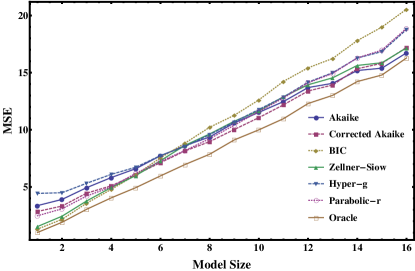
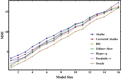
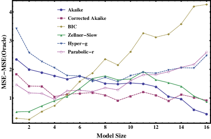
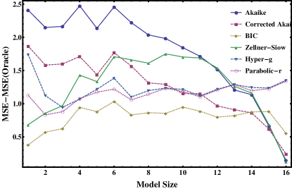
Figure 1: Upper panels: Comparison of MSE values for different model comparison schemes as a function of model size $K$ for weak signal on the left and strong signal on the right. The lower panels show corresponding differences between MSE($K$) and MSE(Oracle).

$K$	Oracle	AIC	AICc	BIC	$\mathcal{H}_{\!\scriptscriptstyle ZS}$	$\mathcal{H}_{g}$	$\mathcal{H}_{r}$
1	1.01	3.37	2.85	1.31	1.53	4.44	2.48
2	1.91	3.91	3.33	2.17	2.44	4.49	3.09
3	3.05	4.94	4.46	3.58	3.77	5.32	4.21
4	4.04	5.82	5.10	4.78	4.95	6.10	5.00
5	4.94	6.60	6.07	6.06	6.00	6.73	6.19
6	5.96	7.73	7.13	7.55	7.30	7.74	7.24
7	6.96	8.61	8.15	8.83	8.64	8.54	8.19
8	7.86	9.37	8.96	10.2	9.63	9.58	9.22
9	9.11	10.6	10.0	11.3	10.7	10.7	10.4
10	10.0	11.5	11.1	12.6	11.7	11.8	11.6
11	11.0	12.5	12.2	14.2	12.9	12.9	12.8
12	12.3	13.7	13.4	15.4	13.9	14.2	14.1
13	13.0	14.1	13.9	16.2	14.5	15.0	14.9
14	14.2	15.2	15.3	17.8	15.6	16.3	16.3
15	14.8	15.4	15.8	19.0	15.9	16.8	17.0
16	16.3	16.7	17.2	20.5	17.2	18.8	18.9

Table 2: Comparison of MSE values for different model comparison schemes as a function of model size $K$ for the weak signal case.

$K$	Oracle	AIC	AICc	BIC	$\mathcal{H}_{\!\scriptscriptstyle ZS}$	$\mathcal{H}_{g}$	$\mathcal{H}_{r}$
1	1.03	3.44	2.90	1.41	1.72	2.77	2.16
2	2.02	4.17	3.60	2.59	2.87	3.14	2.85
3	2.80	4.97	4.40	3.43	3.77	3.75	3.68
4	3.85	6.32	5.56	4.80	5.28	4.92	4.93
5	5.14	7.27	6.58	6.02	6.47	6.36	6.31
6	5.93	8.39	7.70	6.96	7.64	7.31	7.15
7	6.87	9.09	8.44	7.70	8.53	7.98	7.93
8	8.11	10.1	9.42	8.97	9.72	9.30	9.25
9	8.87	10.9	10.2	9.73	10.6	10.1	10.1
10	10.1	11.9	11.3	11.1	11.8	11.3	11.3
11	10.7	12.4	11.8	11.6	12.4	11.8	11.8
12	12.1	13.6	13.1	12.9	13.6	13.3	13.3
13	13.2	14.4	14.1	14.0	14.4	14.5	14.4
14	13.7	14.9	14.6	14.6	14.9	15.0	14.9
15	14.9	15.6	15.5	15.8	15.6	16.1	16.1
16	15.9	16.0	16.1	16.4	16.0	17.2	17.2

Table 3: Comparison of MSE values for different model comparison schemes as a function of model size $K$ for the strong signal case.

5 Discussion

We have introduced in this article the $r$-prior based on explicit enforcement of spherical symmetry on the diagonalised parameter space. The resulting formalism has been shown to encompass the currently popular Zellner $g$-prior, Zellner-Siow Cauchy prior and the hyper-$g$ prior as special cases. Beyond these, we have shown by example of a new parabolic $r$-prior how different considerations such as asymptotic behaviour may be incorporated. Other $r$-priors based on further and different information can presumably be implemented in future.

Conceptually, the $r$-priors appear to be a step towards a more formal understanding of the symmetries on the hypersphere which are implicit in canonical regression problems. The next step would be to understand the scale symmetry governing $r$ itself.

The simulation shows that the $r$-prior gives good results, but also that the detailed behaviour of it and other model schemes is quite variable and poorly understood. Both the type of simulation and the comparison criterion must in future be investigated in some detail.

Acknowledgements: This work is supported in part by a Consolidoc fellowship of Stellenbosch University and by the National Research Foundation of South Africa. We thank the referee for useful comments and suggestions. Thanks also to the organisers of the 2014 ISBA–George Box Research Workshop on Frontiers of Statistics for support and the participants for helpful discussions.

References

• [Akaike, 1974] Akaike, H. (1974). A new look at the statistical model identification. Automatic Control, IEEE Transactions on, 19(6):716–723.
• [Bateman et al., 1953] Bateman, H., Erdélyi, A., Magnus, W., Oberhettinger, F., and Tricomi, F. G. (1953). Higher Transcendental Functions, volume 1. McGraw-Hill New York.
• [Berger et al., 2001] Berger, J. O., Pericchi, L. R., Ghosh, J. K., Samanta, T., and Santis, F. D. (2001). Objective bayesian methods for model selection: Introduction and comparison. Lecture Notes – Monograph Series, 38:pp. 135–207.
• [Box and Tiao, 1973] Box, G. and Tiao, G. (1973). Bayesian Inference in Statistical Analysis. Reading, MA.
• [Bretthorst, 1988] Bretthorst, G. (1988). Bayesian Spectrum Analysis and Parameter Estimation. Lecture notes in statistics. Springer-Verlag.
• [Celeux et al., 2012] Celeux, G., El Anbari, M., Marin, J.-M., and Robert, C. P. (2012). Regularization in regression: Comparing bayesian and frequentist methods in a poorly informative situation. Bayesian Analysis, 7(2):477–502.
• [George and McCulloch, 1997] George, E. I. and McCulloch, R. E. (1997). Approaches for bayesian variable selection. Statistica Sinica, 7(2):339–373.
• [Hurvich and Tsai, 1989] Hurvich, C. M. and Tsai, C.-L. (1989). Regression and time series model selection in small samples. Biometrika, 76(2):297–307.
• [Jaynes, 2003] Jaynes, E. T. (2003). Probability Theory: The Logic of Science (Appendix B). Cambridge University Press.
• [Jeffreys, 1967] Jeffreys, H. (1967). Theory of Probability. International Series of Monographs on Physics. Clarendon Press.
• [Leamer, 1978] Leamer, E. E. (1978). Regression selection strategies and revealed priors. Journal of the American Statistical Association, 73(363):580–587.
• [Liang et al., 2008] Liang, F., Paulo, R., Molina, G., Clyde, M. A., and Berger, J. O. (2008). Mixtures of g-priors for bayesian variable selection. Journal of the American Statistical Association, 103(481).
• [Raftery et al., 1997] Raftery, A. E., Madigan, D., and Hoeting, J. A. (1997). Bayesian model averaging for linear regression models. Journal of the American Statistical Association, 92(437):179–191.
• [Schwarz, 1978] Schwarz, G. (1978). Estimating the dimension of a model. The Annals of Statistics, 6(2):461–464.
• [Watson, 1922] Watson, G. (1922). A Treatise on the Theory of Bessel Functions. The University Press.
• [Zellner, 1971] Zellner, A. (1971). An Introduction to Bayesian Inference in Econometrics. Wiley series in probability and mathematical statistics: Applied probability and statistics. J. Wiley.
• [Zellner, 1986] Zellner, A. (1986). On assessing prior distributions and bayesian regression analysis with g-prior distributions. Bayesian Inference and Decision Techniques: Essays in Honor of Bruno De Finetti, 6:233–243.
• [Zellner and Siow, 1980] Zellner, A. and Siow, A. (1980). Posterior odds ratios for selected regression hypotheses. Trabajos de estadística y de investigación operativa, 31(1):585–603.