A Comparison of Cosmological Models Using Strong Gravitational Lensing Galaxies

Abstract

Strongly gravitationally lensed quasar-galaxy systems allow us to compare competing cosmologies as long as one can be reasonably sure of the mass distribution within the intervening lens. In this paper, we assemble a catalog of 69 such systems from the Sloan Lens ACS and Lens Structure and Dynamics surveys suitable for this analysis, and carry out a one-on-one comparison between the standard model, $\Lambda$CDM, and the $R_{\rm h}=ct$ Universe, which has thus far been favored by the application of model selection tools to other kinds of data. We find that both models account for the lens observations quite well, though the precision of these measurements does not appear to be good enough to favor one model over the other. Part of the reason is the so-called bulge-halo conspiracy that, on average, results in a baryonic velocity dispersion within a fraction of the optical effective radius virtually identical to that expected for the whole luminous-dark matter distribution modeled as a singular isothermal ellipsoid, though with some scatter among individual sources. Future work can greatly improve the precision of these measurements by focusing on lensing systems with galaxies as close as possible to the background sources. Given the limitations of doing precision cosmological testing using the current sample, we also carry out Monte Carlo simulations based on the current lens measurements to estimate how large the source catalog would have to be in order to rule out either model at a $\sim 99.7\%$ confidence level. We find that if the real cosmology is $\Lambda$CDM, a sample of $\sim 200$ strong gravitational lenses would be sufficient to rule out $R_{\rm h}=ct$ at this level of accuracy, while $\sim 300$ strong gravitational lenses would be required to rule out $\Lambda$CDM if the real Universe were instead $R_{\rm h}=ct$. The difference in required sample size reflects the greater number of free parameters available to fit the data with $\Lambda$CDM. We point out that, should the $R_{\rm h}=ct$ Universe eventually emerge as the correct cosmology, its lack of any free parameters for this kind of work will provide a remarkably powerful probe of the mass structure in lensing galaxies, and a means of better understanding the origin of the bulge-halo conspiracy.

1 Introduction

An interesting new idea started emerging a decade ago (see, e.g., Treu et al. 2006; Grillo et al. 2008; Biesiada et al. 2010; but also see Futamase & Yoshida 2001) to use individual lensing galaxies in order to measure cosmological parameters. In principle, the deflection of quasar light by the intervening galaxy is known precisely from general relativity as long as one has a good model for the mass distribution within the lens (Bartelmann & Schneider 1999; Refregier 2003). The Einstein radius, inferred from the deflection angle, then provides a measure of the angular-size distance, which may be used to discriminate between competing cosmological models.

The key, of course, is how well we understand the distribution of matter within the lens, and this appears to be the principal source of error in this type of measurement. As of today, the observation of some 70 or so lensing galaxy systems has provided the data that, in principle, can be used to carry out this kind of study. The results thus far are consistent with the standard ($\Lambda$CDM) model, though the precision with which model parameters may be determined with this appoach is not yet as good as that available in other studies, e.g., using Type Ia SNe as standard candles (see, e.g., Riess et al. 1998; Perlmutter et al. 1999).

In recent years, the application of model selection tools in one-on-one comparisons between $\Lambda$CDM and a cosmology we refer to as the $R_{\rm h}=ct$ Universe (Melia 2007; Melia & Shevchuk 2012) has shown that the data actually tend to favor the latter over the former. These include the use of cosmic chronometers (Melia & Maier 2013), high-$z$ quasars (Melia 2013), gamma ray bursts (Wei et al. 2013) and, most recently, the Type Ia SNe themselves (Wei et al. 2014b). The simplest way to view this cosmology is to start with $\Lambda$CDM and then apply the additional constraint $p=-\rho/3$ on its total equation of state, where $p$ and $\rho$ are the total pressure and energy density, respectively. With these other kinds of data, $R_{\rm h}=ct$ is favored over $\Lambda$CDM with a likelihood of $\sim 90\%$ versus only $\sim 10\%$.

The principal goal of this paper is to broaden the comparison between $R_{\rm h}=ct$ and $\Lambda$CDM by now including strong gravitational lenses in this study. In § 2 of this paper, we describe the method, and then assemble the catalog of suitable lensing systems in § 3. We discuss our results in § 4. We will find that the current strong lensing sample is not yet large enough to differentiate between these two competing models, and we show in § 5 how large the source catalog needs to be in order to rule out one or the other expansion scenarios at a 3-sigma confidence level. We present our conclusions in § 6.

2 Strong Lensing

The lens model often fitted to the observed images is based on a singular isothermal ellipsoid (SIE; Ratnatunga et al. 1999), in which the projected mass distribution (at redshift $z_{l}$) is elliptical, with semi-minor axis $\theta_{1}$ and semi-major axis $\theta_{2}$. In this paper, we will adopt the simpler version, using a singular isothermal sphere instead. For generality, we will describe the approach using semi-major and semi-minor axes, though we will later set the two angles $\theta_{1}$ and $\theta_{2}$ equal to each other. The source lensed by this system is a quasar at redshift $z_{s}>z_{l}$. The key expression in strong gravitational lensing theory is the lens equation (Schneider et al. 1992), which gives the mapping between positions $\beta$ in the source plane and $\theta$ in the image plane, according to

$$\beta=\theta-\nabla_{\theta}\Phi\;.$$ (1)

The lensing potential of the singular isothermal ellipsoid may be written (Kormann et al. 1994)

$$\Phi=\theta_{\rm E}\sqrt{(1-\epsilon)\theta_{1}^{2}+(1+\epsilon)\theta_{2}^{2}}\;,$$ (2)

where the Einstein radius $\theta_{\rm E}$ is defined below in terms of the (one-dimensional) velocity dispersion, $\sigma_{v}$, in the lensing galaxy, and the angular diameter distances, $D_{A}(z_{l},z_{s})$ and $D_{A}(0,z_{s})$, between lens and source and between source and observer, respectively. The ‘ellipticity’ $\epsilon$ is related to the eccentricity $e$ of the critical line by

$$e=\sqrt{(1-\epsilon)/(1+\epsilon)}\;.$$ (3)

In addition, the semi-major and semi-minor axes are related to the Einstein radius

$$\theta_{\rm E}\equiv 4\pi\left({\sigma_{v}\over c}\right)^{2}{\mathcal{D}}\;,$$ (4)

where

$${\mathcal{D}}\equiv{D_{A}(z_{l},z_{s})\over D_{A}(0,z_{s})}\;,$$ (5)

via the relations

$$\theta_{1} = \theta_{\rm E}\sqrt{1-\epsilon}$$

$$\theta_{2} = \theta_{\rm E}\sqrt{1+\epsilon}\;.$$ (6)

As noted, earlier, we will here consider the simpler case of a single isothermal sphere (SIS), for which $\theta_{1}=\theta_{2}$.

In principle, equation (4) can be used to test cosmological models in a rather unique way because, unlike other kinds of comparisons that rely on the optimization of the Hubble constant $H_{0}$, this particular analysis is completely independent of $H_{0}$. Nonetheless, even though knowledge of $H_{0}$ is not necessary for this type of test, fits to the data do depend on the reliability of lens modelling (e.g., via the assumption of a singular isothermal sphere, or a singular isothermal ellipsoid) and the measurement of the velocity dispersion.

When using these expressions, $\sigma_{v}$ (the total velocity dispersion of stellar plus dark matter) cannot be obtained directly from the surface-brightness weighted average of the line-of-sight velocity dispersion that is actually measured. In practice, the central velocity dispersion $\sigma_{0}$ is estimated from the stellar velocity dispersion within $R_{e}/8$, where $R_{e}$ is the optical effective radius (see, e.g., Treu et al. 2006; Grillo et al. 2008), and is then used to represent the velocity dispersion $\sigma_{SIS}$ for the corresponding singular isothermal sphere or ellpisoid (for the total mass present). This works rather well because inside one effective radius, massive elliptical galaxies are kinematically indistinguishable from an isothermal ellipsoid (Koopmans et al. 2009), which is quite remarkable considering the fact that $\sigma_{SIS}$ and $\sigma_{0}$ need not be the same. One reason is that dark matter halos appear to be dynamically hotter than the luminous stars (based on X-ray observations), so the former must necessarily have a greater velocity dispersion than the latter (White & Davis 1996).

Still, when one introduces the SIS equivalent value $\sigma_{SIS}$ obtained from modelling the lens as a singular isothermal sphere, these two measures of velocity dispersion agree very closely. Treu et al. (2006) used the large and homogeneously selected sample of lenses identified by the Sloan Lenses ACS Survey (SLACS; Bolton et al. 2005, 2006) to study in detail the degree of homogeneity of the early-type galaxies by measuring the ratio between stellar velocity dispersion and $\sigma_{SIS}$ that best fits the geometry of the corresponding multiple images. They found that the ratio ${\sigma_{0}/\sigma_{SIS}}$ is very close to unity; specifically, they inferred a sample average value $\langle{\sigma_{0}/\sigma_{SIS}}\rangle=1.010\pm 0.017$, with a relatively small scatter of $\sim 0.06$. Similarly, van de Ven et al. (2003) examined this ratio for a range of anisotropy parameters and found that $0.96<{\sigma_{0}/\sigma_{SIS}}<1.08$. The conclusion from such studies is that on average the approximation $\sigma_{v}=\sigma_{SIS}\approx\sigma_{0}$ works surprisingly well, due perhaps to some as yet unknown mechanism that couples stellar and dark mass, sometimes referred to as a bulge-halo ‘conspiracy’. A possible resolution of this parity may be that since the NFW (Navarro et al. 1997) and observed stellar mass profiles are nearly isothermal, the more concentrated mass profiles for the baryon component than for dark matter may simply be a consequence of dissipative star formation. The observation of $\sigma_{0}/\sigma_{SIS}\sim 1$ may therefore not be so mysterious. Nonetheless, significant departures from this are seen in individual cases, so one cannot ignore the scatter in any discussion concerning the propagated measurement error for ${\mathcal{D}}_{obs}$.

In this paper, we will follow Cao et al. (2012), and put

$$\theta_{\rm E}\equiv 4\pi\left({\sigma_{SIS}\over c}\right)^{2}{\mathcal{D}}\;,$$ (7)

with

$$\sigma_{SIS}\equiv f_{SIS}\,\sigma_{0}\;.$$ (8)

We will keep $f_{SIS}$ as a free parameter to be optimized in the fits, since it mimics at least several effects that apparently give rise to the observed scatter in the individually measured ratio $\sigma_{0}/\sigma_{SIS}$ for each system. These include: (1) systematic errors in the rms deviation of $\sigma_{SIS}$ from $\sigma_{0}$; (2) an rms error associated with the assumption that the SIS model allows the translation from observed image separation to $\theta_{\rm E}$; and (3) a softened isothermal sphere potential, which tends to decrease the typical image separations (Narayan & Bartelmann 1996). In the analysis we describe below, we will adopt a dispersion $\sigma_{f}=0.06\,f_{SIS}$, based on the rms scatter of $\sim 6\%$ found from the work of Treu et al. (2006) and van de Ven et al. (2003). Note, however, that $\sigma_{f}$ may be as big as $\sim 0.2$ according to Cao et al. (2012), though one might have expected such a large value to have emerged directly from the aforementioned survey by Treu et al. (2006).

The overall uncertainty associated with ${\mathcal{D}_{obs}}$ (calculated from equation 7) is estimated through the propagation equation involving errors in $\theta_{\rm E}$, $\sigma_{0}$, and $f_{SIS}$. According to Grillo et al. (2008), the error in measuring the Einstein radius $\theta_{\rm E}$ is $\sim 5\%$, so we will assume a dispersion $\sigma_{\theta_{\rm E}}=0.05\,\theta_{\rm E}$ for this quantity. In principle, any optimization of the model parameters (and $f_{SIS}$) carried out while fitting the data should also include the dispersion $\sigma_{z}$ in the measured redshifts $z_{l}$ and $z_{s}$ (since the theoretical values $D_{A}(z_{l},z_{s})$ and $D_{A}(0,z_{s})$ directly depend on these). However, a careful analysis of SDSS quasar spectra shows that $\sigma_{z}/(1+z)\sim 10^{-4}$ over a broad range of redshifts (Hewett & Wild 2010). This error is so small compared to the other three uncertainties that we will ignore it. So in total, we will calculate the dispersion $\sigma_{\mathcal{D}}$ in ${\mathcal{D}_{obs}}$ using the expression

$$\sigma_{\mathcal{D}}={\mathcal{D}_{obs}}\left[\left({\sigma_{\theta_{\rm E}}\over\theta_{\rm E}}\right)^{2}+4\left({\sigma_{\sigma_{0}}\over\sigma_{0}}\right)^{2}+4\left({\sigma_{f}\over f_{SIS}}\right)^{2}\right]^{1/2}\;.$$ (9)

Note that since the uncertainty in $\sigma_{0}$ also appears to be $\sim 5\%$ (Grillo et al. 2008), the average dispersion in the measured value of $\mathcal{D}$ is expected to be $\sigma_{\mathcal{D}}\sim 0.16\,{\mathcal{D}_{obs}}$.

Now, in principle, only the range $0\leq{\mathcal{D}}\leq 1$ is physically meaningful, but such a value of $\sigma_{\mathcal{D}}$ can result in at least some measurements ${\mathcal{D}_{obs}}>1.0$. A quick inspection of equation (5) shows that the measurements most at risk for this type of outcome involve lenses much closer to the observer than the source. As we shall see below, several of the sources in our complete sample have ${\mathcal{D}_{obs}}>1.0$. Though unrealistic, such values are consistent with the quoted error, so we will include them in our analysis. But to demonstrate their negative impact on the optimization of the model fits, we will also carry out the analysis for a reduced sample omitting these sources. As the measurements become more precise, and the sample of strong lensing sources grows, it may be possible to avoid systems with ${\mathcal{D}_{obs}}>1.0$ altogether.

From a theoretical standpoint, one must assume a cosmological model in order to calculate the angular diameter distances $D_{A}(z_{l},z_{s})$ and $D_{A}(0,z_{s})$, once the redshifts $z_{l}$ and $z_{s}$ for a particular lensing system are known. In $\Lambda$CDM, this distance depends on several parameters, including $H_{0}$ and the mass fractions $\Omega_{\rm m}\equiv\rho_{\rm m}/\rho_{\rm c}$, $\Omega_{\rm r}\equiv\rho_{\rm r}/\rho_{\rm c}$, and $\Omega_{\rm de}\equiv\rho_{\rm de}/\rho_{\rm c}$, defined in terms of the current matter ($\rho_{\rm m}$), radiation ($\rho_{\rm r}$), and dark energy ($\rho_{\rm de}$) densities, and the critical density $\rho_{\rm c}\equiv 3c^{2}H_{0}^{2}/8\pi G$. Assuming zero spatial curvature, so that $\Omega_{\rm m}+\Omega_{\rm r}+\Omega_{\rm de}=1$, the angular diameter distance between redshifts $z_{1}$ and $z_{2}$ ($>z_{1}$) is given by the expression

$$D_{A}^{\Lambda{\rm CDM}}(z_{1},z_{2})={c\over H_{0}}{1\over(1+z_{2})}\int_{z_{1}}^{z_{2}}\left[\Omega_{\rm m}(1+z)^{3}+\Omega_{\rm r}(1+z)^{4}+\Omega_{\rm de}(1+z)^{3(1+w_{\rm de})}\right]^{-1/2}\;dz\;,$$ (10)

where $p_{\rm de}=w_{\rm de}\rho_{\rm de}$ is the dark-energy equation of state. As noted earlier, $H_{0}$ cancels out when we divide $D_{A}^{\Lambda{\rm CDM}}(z_{l},z_{s})$ by $D_{A}^{\Lambda{\rm CDM}}(0,z_{s})$ to form the ratio $\mathcal{D}_{\Lambda{\rm CDM}}$, so the essential remaining parameters in flat $\Lambda$CDM are $\Omega_{\rm m}$ and $w_{\rm de}$. If we further assume that dark energy is a cosmological constant with $w_{\rm de}=-1$, then only the parameter $\Omega_{\rm m}$ is available to fit the data.

In the $R_{\rm h}=ct$ Universe (Melia 2007; Melia & Shevchuk 2012), the angular diameter distance depends only on $H_{0}$, but since here too the Hubble constant cancels out in the ratio $\mathcal{D}_{R_{\rm h}=ct}$, there are actually no free parameters left for fitting the gravitational lensing data. In this cosmology,

$$D_{A}^{R_{\rm h}=ct}(z_{1},z_{2})={c\over H_{0}}{1\over(1+z_{2})}\ln\left({1+z_{2}\over 1+z_{1}}\right)\;.$$ (11)

3 Strong Gravitational Lensing Systems

Our sample is drawn from a compilation of 69 strong lensing systems (listed in Table I), with good spectroscopic measurements of the central velocity dispersion, using the SLACS (Sloan Lens ACS) Survey (first introduced by Bolton et al. 2006; Treu et al. 2006; and Koopmans et al. 2006), and the LSD (Lenses Structure and Dynamics) Survey (see, e.g., Bolton et al. 2008; Newton et al. 2011). Some original contributions to these data sets may be found in Young et al. (1980), Huchra et al. (1985), Lehár et al. (1993), Fassnacht et al. (1996), Tonry et al. (1998), Koopmans & Treu (2002, 2003), and Treu and Koopmans (2004). The velocity dispersion $\sigma_{0}$ and its uncertainty (with the aforementioned average value of $\sim 5\%$) were obtained from the Sloan Digital Sky Survey Database. The SLACS and LENS surveys complement each other rather well, with the former comprised primarily of lens galaxies at redshift up to $\sim 0.3$, while the latter includes systems beyond $z\sim 0.5$.

It has already been noted before (see, e.g., Biesiada et al. 2010, 2011; Cao et al. 2012) that some of these lenses produce 2 images, while others produce 4. Both 2-image and 4-image lens systems are usually affected by external shear. This effect degenerates with the ellipticity of the SIE component, which introduces some uncertainty in estimating the Einstein radius of a given lens. For 2-image systems this can be more problematic due to a lack of observational constraints. On the other hand, 4-image systems are better constrained observationally, so both their ellipticity and external shear may be determined for a more accurate measurement of the Einstein radius. To gauge whether there are any systematic effects associated with one category or the other, we will here track the results using both sets of lens system.

There is an additional drawback to the measurement of $\mathcal{D}$ with strong gravitational lenses that we must carefully consider here. By its very definition, $\mathcal{D}$ is confined to a very compact range of values $(0,1)$, regardless of the lens ($z_{l}$) and quasar ($z_{s}$) redshifts. In addition, there is no monotonic progression from low to high values of $\mathcal{D}$ as the sequence of gravitational lenses approaches or recedes from us, since the sources may lie anywhere beyond them. Fortunately, $\mathcal{D}$ does not depend on $H_{0}$, so a comparison between theoretical values of this ratio and $\mathcal{D}_{\rm obs}$ is not inhibited by any uncertainty in the expansion rate itself. However, the tight range in $\mathcal{D}$ and its lack of correlation with $z$ make it difficult to optimize parameters such as $\Omega_{\rm m}$, which produce only slight changes in $\mathcal{D}_{\Lambda{\rm CDM}}$ even when they increase by a factor of 2 or more. In this paper, we will therefore compare how well $R_{\rm h}=ct$ fits the data with several specific variations of $\Lambda$CDM, though always assuming a flat spatial curvature and a cosmological constant with $w_{\rm de}=-1$. The most prominent

Table 1: Strong Gravitational Lensing Systems

Galaxy	$z_{l}$	$z_{s}$	$\theta_{\rm E}$	$\sigma_{0}$	$\mathcal{D}_{\rm obs}$	$\sigma_{\mathcal{D}}$	${\mathcal{D}_{R_{\rm h}=ct}}$	${\mathcal{D}_{\Lambda{\rm CDM}}}$	Refs.
			(arcsec)	(${\rm km}\;{\rm s}^{-1})$	$f_{\rm SIS}=1.02$			$(\Omega_{\rm m}=0.27)$
Systems with Two Images
SDSS J0037-0942	0.1955	0.6322	1.47	282$\pm$11	0.617	0.094	0.636	0.656	1–9
SDSS J0216-0813	0.3317	0.5235	1.15	349$\pm$24	0.316	0.060	0.320	0.336	1–9
SDSS J0737+3216	0.3223	0.5812	1.03	326$\pm$16	0.323	0.053	0.390	0.409	1–9
SDSS J0912+0029	0.1642	0.3240	1.61	325$\pm$12	0.509	0.076	0.458	0.474	1–9
SDSS J1250+0523	0.2318	0.7950	1.15	274$\pm$15	0.511	0.087	0.644	0.665	1–9
SDSS J1630+4520	0.2479	0.7933	1.81	279$\pm$17	0.776	0.138	0.621	0.642	1–9
SDSS J2300+0022	0.2285	0.4635	1.25	305$\pm$19	0.448	0.081	0.460	0.479	1–9
SDSS J2303+1422	0.1553	0.5170	1.64	271$\pm$16	0.745	0.131	0.654	0.673	1–9
CFRS03.1077	0.9380	2.9410	1.24	251$\pm$19	0.657	0.131	0.518	0.506	1–9
HST 15433	0.4970	2.0920	0.36	116$\pm$10	0.893	0.193	0.643	0.652	1–9
MG2016	1.004	3.263	1.56	328$\pm$32	0.484	0.113	0.521	0.504	1–9
SDSS J0044+0113	0.1196	0.1965	0.79	266$\pm$13	0.373	0.061	0.370	0.381	10,11
SDSS J0330-0020	0.3507	1.0709	1.10	212$\pm$21	0.817	0.194	0.587	0.608	10,11
SDSS J0935-0003	0.3475	0.4670	0.87	396$\pm$35	0.185	0.041	0.222	0.234	10,11
SDSS J0955+0101	0.1109	0.3159	0.91	192$\pm$13	0.824	0.155	0.617	0.632	10,11
SDSS J0959+4416	0.2369	0.5315	0.96	244$\pm$19	0.538	0.109	0.501	0.521	10
SDSS J1112+0826	0.2730	0.6295	1.48	320$\pm$20	0.486	0.088	0.506	0.527	10,11
SDSS J1142+1001	0.2218	0.5039	0.98	221$\pm$22	0.670	0.159	0.509	0.529	10,11
SDSS J1143-0144	0.1060	0.4019	1.68	269$\pm$13	0.775	0.126	0.702	0.718	10
SDSS J1204+0358	0.1644	0.6307	1.31	267$\pm$17	0.613	0.112	0.689	0.708	10,11
SDSS J1205+4910	0.2150	0.4808	1.22	281$\pm$14	0.516	0.084	0.504	0.524	10
SDSS J1213+6708	0.1229	0.6402	1.42	292$\pm$15	0.556	0.092	0.766	0.783	10,11
SDSS J1403+0006	0.1888	0.4730	0.83	213$\pm$17	0.611	0.126	0.553	0.573	10
SDSS J1436-0000	0.2852	0.8049	1.12	224$\pm$17	0.745	0.149	0.575	0.597	10,11
SDSS J1443-0304	0.1338	0.4187	0.81	209$\pm$11	0.619	0.104	0.641	0.658	10,11
SDSS J1451-0239	0.1254	0.5203	1.04	223$\pm$14	0.698	0.126	0.718	0.735	10,11
SDSS J1525+3327	0.3583	0.7173	1.31	264$\pm$26	0.627	0.148	0.434	0.454	10,11
SDSS J1531-0105	0.1596	0.7439	1.71	279$\pm$14	0.733	0.120	0.734	0.753	10,11
SDSS J1538+5817	0.1428	0.5312	1.00	189$\pm$12	0.934	0.170	0.687	0.705	10,11
SDSS J1621+3931	0.2449	0.6021	1.29	236$\pm$20	0.773	0.165	0.535	0.556	10,11
MG1549+3047	0.11	1.17	1.15	227$\pm$18	0.745	0.153	0.865	0.878	12
CY2201-3201	0.32	3.90	0.41	130$\pm$20	0.810	0.270	0.825	0.764	2,4,5
SDSS J1432+6317	0.1230	0.6643	1.26	199$\pm$10	1.062	0.174	0.772	0.749	10,11
SDSS J2238-0754	0.1371	0.7126	1.27	198$\pm$11	1.081	0.185	0.761	0.736	10,11
Q0957+561	0.36	3.90	1.41	167$\pm$10	1.077	0.190	0.650	0.599	13
Systems with More than Two Images
SDSS J0956+5100	0.2405	0.4700	1.32	318$\pm$17	0.436	0.073	0.441	0.459	1–9
SDSS J0959+0410	0.1260	0.5349	1.00	229$\pm$13	0.636	0.110	0.723	0.740	1–9
SDSS J1330-0148	0.0808	0.7115	0.85	195$\pm$10	0.746	0.124	0.855	0.868	1–9
SDSS J1402+6321	0.2046	0.4814	1.39	290$\pm$16	0.552	0.094	0.526	0.546	1–9
SDSS J1420+6019	0.0629	0.5352	1.04	206$\pm$5	0.818	0.113	0.858	0.869	1–9
SDSS J1627-0053	0.2076	0.5241	1.21	295$\pm$13	0.464	0.073	0.552	0.573	1–9
SDSS J2321-0939	0.0819	0.5324	1.57	245$\pm$7	0.873	0.124	0.816	0.829	1–9
Q0047-2808	0.4850	3.5950	1.34	229$\pm$15	0.853	0.157	0.741	0.738	1–9
HST 14176	0.8100	3.3990	1.41	224$\pm$15	0.938	0.175	0.599	0.587	1–9
SDSS J0029-0055	0.2270	0.9313	0.96	229$\pm$18	0.611	0.125	0.689	0.710	10,11
SDSS J0109+1500	0.2939	0.5248	0.69	251$\pm$19	0.366	0.073	0.389	0.407	10
SDSS J0728+3835	0.2058	0.6877	1.25	214$\pm$11	0.911	0.151	0.642	0.663	10,11
SDSS J0822+2652	0.2414	0.5941	1.17	259$\pm$15	0.582	0.101	0.536	0.557	10,11
SDSS J0841-3824	0.1159	0.6567	1.41	225$\pm$11	0.930	0.151	0.783	0.799	10,11
SDSS J0936+0913	0.1897	0.5880	1.09	243$\pm$12	0.616	0.101	0.624	0.645	10
SDSS J0946+1006	0.2219	0.6085	1.38	263$\pm$21	0.666	0.137	0.609	0.599	10,11
SDSS J1016+3859	0.1679	0.4349	1.09	247$\pm$13	0.596	0.100	0.570	0.589	10
SDSS J1020+1122	0.2822	0.5530	1.20	282$\pm$18	0.504	0.092	0.435	0.455	10
SDSS J1023+4230	0.1912	0.6960	1.41	242$\pm$15	0.804	0.144	0.669	0.808	10,11
SDSS J1029+0420	0.1045	0.6154	1.01	210$\pm$11	0.764	0.128	0.793	0.808	10
SDSS J1032+5322	0.1334	0.3290	1.03	296$\pm$15	0.392	0.065	0.560	0.576	10
SDSS J1103+5322	0.1582	0.7353	1.02	196$\pm$12	0.886	0.158	0.734	0.752	10,11
SDSS J1106+5228	0.0955	0.4069	1.23	262$\pm$13	0.598	0.098	0.733	0.748	10,11
SDSS J1134+6027	0.1528	0.4742	1.10	239$\pm$12	0.643	0.106	0.634	0.652	10
SDSS J1153+4612	0.1797	0.8751	1.05	226$\pm$15	0.686	0.127	0.737	0.756	10
SDSS J1416+5136	0.2987	0.8111	1.37	240$\pm$25	0.794	0.195	0.560	0.582	10,11
SDSS J1430+4105	0.2850	0.5753	1.52	322$\pm$32	0.489	0.116	0.448	0.468	10
SDSS J1636+4707	0.2282	0.6745	1.09	231$\pm$15	0.682	0.125	0.601	0.623	10
PG1115+080	0.3100	1.7200	1.21	281$\pm$25	0.511	0.113	0.730	0.745	14
Q2237+030	0.04	1.169	0.91	215$\pm$30	0.657	0.202	0.949	0.940	15
B1608+656	0.63	1.39	1.13	247$\pm$35	0.618	0.193	0.439	0.386	16
SDSS J0252+0039	0.2803	0.9818	1.04	164$\pm$12	1.290	0.253	0.639	0.599	10
SDSS J0405-0455	0.0753	0.8098	0.80	160$\pm$8	1.043	0.171	0.878	0.861	10
SDSS J2341+0000	0.186	0.807	1.44	207$\pm$13	1.122	0.203	0.712	0.681	10,11

comparison will be between $R_{\rm h}=ct$ and the concordance model (with $\Omega_{\rm m}=0.27$), though we will also consider other values of $\Omega_{\rm m}$, including the Einstein-de Sitter (E-deS) model with $\Omega_{\rm m}=1$.

Related to the possible difficulty in using sources with $\mathcal{D}_{\rm obs}>1$ is the fact that the uncertainty $\sigma_{\mathcal{D}}$ in $\mathcal{D}_{\rm obs}$ carries significantly more weight when $\mathcal{D}_{\rm obs}\gtrsim 0.6$ than elsewhere in its permitted range, because here big changes in $z_{s}$ produce only very slight modifications to $\mathcal{D}_{\Lambda{\rm CDM}}$ and $\mathcal{D}_{R_{\rm h}=ct}$. One therefore sees an increasing scatter among the observed values of $\mathcal{D}_{\rm obs}$, as shown in figures 1 and 2. In order to fully understand the impact of all of these issues, we will analyze the quality of the theoretical fit for both the full sample and a reduced sample with $\mathcal{D}_{\rm obs}<1$, and in each case also a sub-sample of 2-image systems only. Figures 1 and 2 show the results of analyzing all lensing systems with 2 images only. The figures corresponding to other sample selection criteria are very similar.

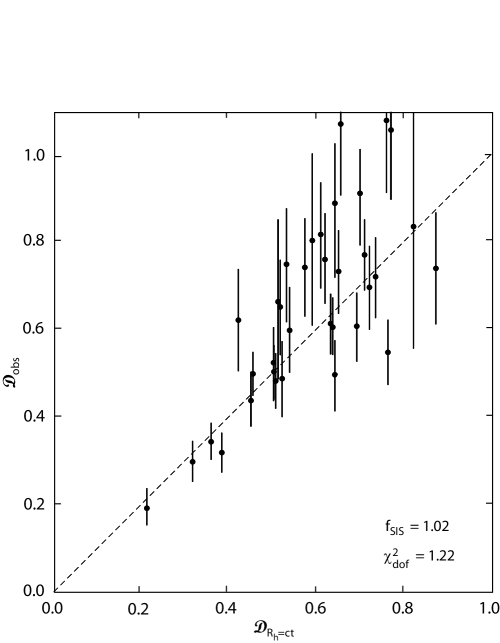
Figure 1: Observed value of $\mathcal{D}$ versus that predicted in the $R_{\rm h}=ct$ Universe for all lensing systems with 2 images only. A perfect fit would correspond to the dashed diagonal line. The optimized value of $f_{\rm SIS}$ in this case is $1.02$, and the reduced $\chi^{2}$ is $1.22$, with $34-1=33$ degrees of freedom.

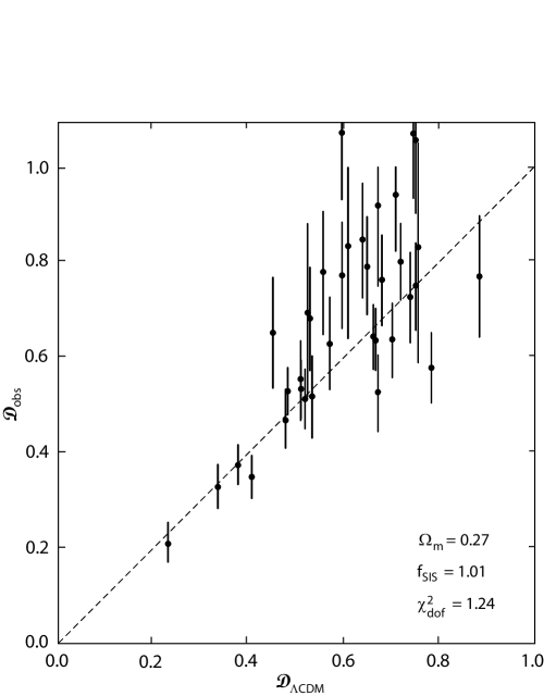
Figure 2: Same as figure 1, except now for the concordance $\Lambda$CDM model, with $\Omega_{\rm m}=0.27$. The optimized value of $f_{\rm SIS}$ is $1.004$, and the reduced $\chi^{2}$ for this fit is $1.24$, with $34-1=33$ degrees of freedom.

As we have already noted, the power to optimize model parameters, such as $\Omega_{\rm m}$ in a multi-parameter context, is very limited (Biesiada et al. 2010; Cao et al. 2012). This will become quite apparent in our discussion below, where we compare the quality of the fit for several variations of $\Lambda$CDM. For each model we consider here, we will therefore optimize the fit using only $f_{\rm SIS}$ as a free parameter, which we do by minimizing the $\chi^{2}$ function

$$\chi^{2}(f_{\rm SIS})=\sum_{i}{\left(\mathcal{D}_{{\rm obs},i}[f_{\rm SIS}]-\mathcal{D}_{{\rm th},i}\right)^{2}\over\sigma_{\mathcal{D},i}^{2}}\;,$$ (12)

where the index $i$ runs over all lens systems in the sample, ‘th’ stands for either $\Lambda$CDM or $R_{\rm h}=ct$, and $\sigma_{\mathcal{D},i}^{2}$ is the variance of $\mathcal{D}_{{\rm obs},i}$ calculated from equation (9).

4 Discussion

We have used the data shown in Table 1 to compare 3 variations of $\Lambda$CDM and the $R_{\rm h}=ct$ Universe, though always for a flat universe ($k=0$) and $w_{\rm de}=-1$. A summary of the results is provided in Tables 2 and 3 for the whole sample (of 69 sources), and in Tables 4 and 5 for a reduced sample with $\mathcal{D}_{\rm obs}<1$ only (63 systems). We note, first of all, that the optimized value of $f_{\rm SIS}$ is very close to 1 in every case, in complete agreement with earlier findings, e.g., by Treu et al. (2006), and van de Ven et al. (2003). As such, we do not find any possible dependence of the so-called bulge-halo ‘conspiracy’ on the assumed cosmological model.

Table 2: Model Comparison for the Whole Sample

Model	$\qquad\Omega_{\rm m}\qquad$	$\qquad f_{\rm SIS}\qquad$	$\qquad\chi^{2}_{\rm dof}\qquad$
$R_{\rm h}=ct$	….	1.023	1.22
$\Lambda$CDMa	0.20	1.00	1.22
Concordancea	0.27	1.01	1.24
Einstein-de Sitter	1.00	1.046	1.33

Table 3: Model Comparison for Two-image Sources

Model	$\qquad\Omega_{\rm m}\qquad$	$\qquad f_{\rm SIS}\qquad$	$\qquad\chi^{2}_{\rm dof}\qquad$
$R_{\rm h}=ct$	….	1.033	1.27
$\Lambda$CDMa	0.20	1.01	1.28
Concordancea	0.27	1.02	1.29
Einstein-de Sitter	1.00	1.059	1.33

Table 4: Model Comparison for all $\mathcal{D}_{\rm obs}<1$

Model	$\qquad\Omega_{\rm m}\qquad$	$\qquad f_{\rm SIS}\qquad$	$\qquad\chi^{2}_{\rm dof}\qquad$
$R_{\rm h}=ct$	….	1.01	0.99
$\Lambda$CDMa	0.20	0.99	0.99
Concordancea	0.27	1.00	1.00
Einstein-de Sitter	1.00	1.03	1.09

Table 5: Model Comparison for 2-images and $\mathcal{D}_{\rm obs}<1$

Model	$\qquad\Omega_{\rm m}\qquad$	$\qquad f_{\rm SIS}\qquad$	$\qquad\chi^{2}_{\rm dof}\qquad$
$R_{\rm h}=ct$	….	1.02	0.92
$\Lambda$CDMa	0.20	1.00	0.92
Concordancea	0.27	1.00	0.93
Einstein-de Sitter	1.00	1.05	0.99

We have compared the model fits using both the full sample of 69 entries in Table 1 and, separately, using only the sub-sample of 34 2-image systems. The quality of the fit, for every model we considered, is actually somewhat better for the former. This may simply be a reflection of the fact that, though technically an isothermal sphere should produce only 2 images, the other possible effects described in § 2 could be significant enough to result in a considerable scatter about the average value $f_{\rm SIS}\sim 1$ for individual systems, that dwarfs all the other possible sources of error in calculating $\mathcal{D}_{\rm obs}$. Indeed, Cao et al. (2012) have argued that $\sigma_{f}$ could be as large as $\sim 20\%$, and even though such a large scatter was not seen by Treu et al. (2006) and van de Ven et al. (2003), they nonetheless did report an rms deviation of at least $6-7\%$.

Given the universal result $f_{\rm SIS}\sim 1$, the entries in column 6 of Table 1 are shown for only one value ($f_{\rm SIS}=1.02$) of this fraction, corresponding to the optimized fit for the $R_{\rm h}=ct$ model using only the 2-image lens systems (with $\mathcal{D}_{\rm obs}<1$). Also, column 9 shows the entries for $\mathcal{D}_{\Lambda{\rm CDM}}$ only for the concordance model, i.e., for $\Omega_{\rm m}=0.27$. These values change somewhat for other choices of $\Omega_{\rm m}$, but not enough to warrant showing all of them here.

Figures 1 and 2 demonstrate graphically how the observed values of $\mathcal{D}$ compare with those predicted by $R_{\rm h}=ct$ and the concordance model using only the sub-sample of 2-image lens systems, but for all values of $\mathcal{D}_{\rm obs}$. The optimized value of $f_{\rm SIS}$ is $1.02$ for the former, and $1.01$ for the latter, and the reduced $\chi^{2}_{\rm dof}$ (with $34-1=33$ degrees of freedom) is quite similar for these two cases, i.e., $1.22$ for the former versus $1.24$ for the latter. It is quite evident from these figures that the scatter in $\mathcal{D}_{\rm obs}$ about the theoretical curves (the straight dashed lines in these plots) increases significantly as $D_{A}(z_{l},z_{s})\rightarrow D_{A}(0,z_{s})$. In other words, it appears that measuring $\mathcal{D}$ becomes progressively less precise as the distance to the gravitational lens becomes a smaller and smaller fraction of the distance to the quasar source. This may simply have to do with the fact that $\theta_{\rm E}$ changes less and less for large values of $z_{s}/z_{l}$ so, for the same error in the Einstein angle, one gets less precision in the measurement of $\mathcal{D}_{\rm obs}/\mathcal{D}_{\rm th}$.

The principal results of this paper are summarized in Tables 2, 3, 4 and 5. The first two show how well the 4 models considered here fit the complete sample of 69 lens systems in Table 1 (for all values of $\mathcal{D}_{\rm obs}$), whereas the latter two give the corresponding results for the reduced sample with $\mathcal{D}_{\rm obs}<1$. Based on the general trends emerging from these numbers, it is safe to draw the following conclusions: (1) Even though the power of $\mathcal{D}$ to discriminate between different values of $\Omega_{\rm m}$ in $\Lambda$CDM is quite limited, this analysis indicates that values larger than $\Omega_{\rm m}=0.27$ probably don’t work as well as those below it, though the differences in $\chi^{2}_{\rm dof}$ are still too small to draw any firm conclusions. And (2), the $R_{\rm h}=ct$ fits the strong gravitational lens data at least as well as $\Lambda$CDM. Still, the differences between $R_{\rm h}=ct$ and $\Lambda$CDM are small enough that one cannot choose one model over the other based solely on this analysis, using the current sample of strong gravitational lens systems. The other tests we have completed thus far, using, e.g., cosmic chronometers (Melia & Maier 2013), high-$z$ quasars (Melia 2013), and gamma ray bursts (Wei et al. 2013), have all resulted in a clear preference for $R_{\rm h}=ct$ over $\Lambda$CDM using statistical model selection tools. The analysis of the strong gravitational lensing data does not result in a comparable outcome yet, though it too does not provide any evidence that the standard model is a better fit to these observations than $R_{\rm h}=ct$.

5 Monte Carlo Simulations with a Mock Sample

In order to provide a detailed quantitative assessment of what kind of strong lensing data are necessary to really distinguish the $R_{\rm h}=ct$ Universe from the standard $\Lambda$CDM model, we will here produce mock samples of strong gravitational lenses based on the current measurement accuracy. Several information criteria commonly used to differentiate between different cosmological models (see, e.g., Melia & Maier 2013, and references cited therein) include the Akaike Information Criterion, ${\rm AIC}=\chi^{2}+2n$, where $n$ is the number of free parameters (Liddle 2007), the Kullback Information Criterion, ${\rm KIC}=\chi^{2}+3n$ (Cavanaugh 2004), and the Bayes Information Criterion, ${\rm BIC}=\chi^{2}+(\ln N)n$, where $N$ is the number of data points (Schwarz 1978). In the case of AIC, with ${\rm AIC}_{\alpha}$ characterizing model $\mathcal{M}_{\alpha}$, the unnormalized confidence that this model is true is the Akaike weight $\exp(-{\rm AIC}_{\alpha}/2)$. Model $\mathcal{M}_{\alpha}$ has likelihood

$$P(\mathcal{M}_{\alpha})=\frac{\exp(-{\rm AIC}_{\alpha}/2)}{\exp(-{\rm AIC}_{1}/2)+\exp(-{\rm AIC}_{2}/2)}$$ (13)

of being the correct choice in this one-on-one comparison. Thus, the difference $\Delta\rm AIC\equiv{\rm AIC}_{2}\nobreak-{\rm AIC}_{1}$ determines the extent to which $\mathcal{M}_{1}$ is favoured over $\mathcal{M}_{2}$. For Kullback and Bayes, the likelihoods are defined analogously. In using the model selection tools, the outcome $\Delta\equiv$ AIC${}_{1}-$ AIC₂ (and analogously for KIC and BIC) is judged ‘positive’ in the range $\Delta=2-6$, ‘strong’ for $\Delta=6-10$, and ‘very strong’ for $\Delta>10$. In this section, we will estimate the sample size required to significantly strengthen the evidence in favour of $R_{\rm h}=ct$ or $\Lambda$CDM, by conservatively seeking an outcome even beyond $\Delta\simeq 11.62$, i.e., we will see what is required to produce a likelihood $\sim 99.7\%$ versus $\sim 0.3\%$, corresponding to a $3\sigma$ confidence level.

We will consider two cases: one in which the background cosmology is assumed to be $\Lambda$CDM, and a second in which it is $R_{\rm h}=ct$, and we will attempt to estimate the number of strong gravitational lenses required in each case in order to rule out the alternative (incorrect) model at a $\sim 99.7\%$ confidence level. The synthetic strong gravitational lenses are each characterized by a set of parameters denoted as ($z_{l}$, $z_{s}$, $\sigma_{SIS}$, $\theta_{\rm E}$). We generate the synthetic sample using the following procedure:

1. The simulations are carried out based on the current lens measurements. We assign the lens redshift $z_{l}$ uniformly between $0.1$ and $1.1$, the source redshift $z_{s}$ uniformly between $1.5$ and $3.5$, and the velocity dispersion $\sigma_{SIS}$ uniformly between $100$ and $300$ km $\rm s^{-1}$, as Paraficz & Hjorth (2009) did in their simulations.

2. With the mock $z_{l}$, $z_{s}$ and $\sigma_{SIS}$, we first infer $\theta_{\rm E}$ from Equation (7) corresponding either to the $R_{\rm h}=ct$ Universe (§ 5.1) or a flat $\Lambda$CDM cosmology with $\Omega_{\rm m}=0.27$ (§ 5.2). We then assign a deviation ($\Delta\theta_{\rm E}$) to the $\theta_{\rm E}$ value, i.e., we infer $\theta^{\prime}_{\rm E}$ from a normal distribution whose center value is $\theta_{\rm E}$, with a dispersion $\sigma=0.12\;\theta_{\rm E}$. The typical value of $\sigma$ is taken from the current (observed) sample, which yields a mean and median deviation of $\sigma=0.15\;\theta_{\rm E}$ and $\sigma=0.11\;\theta_{\rm E}$, respectively. We constrain the mock sample to easily detectable systems, so we include in the simulations only lenses with $\theta^{\prime}_{\rm E}$ larger than $0.1$ arcsec.

Figure 3: Left: “Observed” values of $\mathcal{D}$ versus that predicted in the best-fit $\Lambda$CDM model. A perfect fit would correspond to the dashed diagonal line. The optimized values of $\Omega_{\rm m}$ and $\Omega_{\rm de}$ in this case are $0.45$ and $0.69$, respectively, and the reduced $\chi^{2}$ is $1.32$, with $300-2=298$ degrees of freedom. Right: The $1\sigma-3\sigma$ contours corresponding to the parameters $\Omega_{\rm m}$ and $\Omega_{\rm de}$ in the best-fit $\Lambda$CDM model, using the simulated sample with 300 lens systems, assuming $R_{\rm h}=ct$ as the background cosmology.

3. Assign observational errors to $\sigma_{SIS}$ and $\theta^{\prime}_{\rm E}$. Since both the observed errors $\sigma_{\sigma_{SIS}}$ and $\sigma_{\theta_{\rm E}}$ are about $5\%$ of $\sigma_{SIS}$ and $\theta^{\prime}_{\rm E}$, we will assign the dispersions $\sigma_{\sigma_{SIS}}=0.05\;\sigma_{SIS}$ and $\sigma_{\theta_{\rm E}}=0.05\;\theta^{\prime}_{\rm E}$ to the synthetic sample.

This sequence of steps is repeated for each lens system in the sample, which is enlarged until the likelihood criterion discussed above is reached. As with the real 60-lens sample, we optimize the model fits by minimizing the $\chi^{2}$ function in Equation (12).

5.1 Assuming $R_{\rm h}=ct$ as the Background Cosmology

We have found that a sample of at least 300 strong gravitational lenses is required in order to rule out $\Lambda$CDM at the $\sim 99.7\%$ confidence level, if the background cosmology is in fact $R_{\rm h}=ct$. The left-hand panel of Figure 3 show how the “observed” values of $\mathcal{D}$ compare with those predicted by the best-fit $\Lambda$CDM model using the simulated sample with 300 lens systems, assuming $R_{\rm h}=ct$ as the background cosmology. The optimized parameters corresponding to the best-fit $\Lambda$CDM model for these simulated data are displayed in the right-hand panel of Figure 3. To allow for the greatest flexibility in this fit, we relax the assumption of flatness and allow $\Omega_{\rm de}$ to be a free parameter along with $\Omega_{\rm m}$. The right-hand panel of Figure 3 shows the 2-D plots for the $1\sigma-3\sigma$ confidence regions for $\Omega_{\rm m}$ and $\Omega_{\rm de}$. The best-fit values for $\Lambda$CDM using the simulated sample with 300 lens systems in the $R_{\rm h}=ct$ Universe are $\Omega_{\rm m}=0.45_{-0.24}^{+0.37}$ $(1\sigma)$ and $\Omega_{\rm de}=0.69_{-0.06}^{+0.07}$ $(1\sigma)$, with a $\chi^{2}$ per degree of freedom of $\chi^{2}_{\rm dof}=394.04/298=1.32$.

           

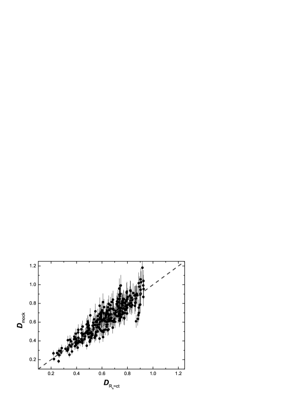
Figure 4: “Observed” values of $\mathcal{D}$ versus that predicted in the $R_{\rm h}=ct$ universe, using a sample of 300 lens systems, simulated with $R_{\rm h}=ct$ as the background cosmology. A perfect fit would correspond to the dashed diagonal line.

In Figure 4, we show how the “observed” values of $\mathcal{D}$ compare with those predicted in the $R_{\rm h}=ct$ universe. Note that there are no free parameters in $R_{\rm h}=ct$. With 300 degrees of freedom, the reduced $\chi^{2}$ is $\chi^{2}_{\rm dof}=394.01/300=1.31$.

Since the number $N$ of data points in the sample is now much greater than one, the most appropriate information criterion to use is the BIC. The logarithmic penalty in this model selection tool strongly suppresses overfitting if $N$ is large (the situation we have here, which is deep in the asymptotic regime). With $N=300$, our analysis of the simulated sample shows that the BIC would favour the $R_{\rm h}=ct$ Universe over $\Lambda$CDM by the aforementioned likelihood of $99.7\%$ versus only $0.3\%$ (i.e., the prescribed $3\sigma$ confidence limit).

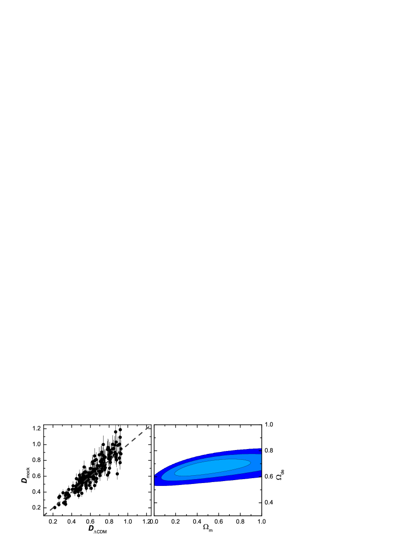
Figure 5: Same as Figure 3, except now with a flat $\Lambda$CDM as the (assumed) background cosmology. The simulated model parameter was $\Omega_{\rm m}=0.27$.

5.2 Assuming $\Lambda$CDM as the Background Cosmology

In this case, we assume that the background cosmology is $\Lambda$CDM, and seek the minimum sample size to rule out $R_{\rm h}=ct$ at the $3\sigma$ confidence level. We have found that a minimum of 200 strong gravitational lenses are required to achieve this goal. To allow for the greatest flexibility in the $\Lambda$CDM fit, here too we relax the assumption of flatness and allow $\Omega_{\rm de}$ to be a free parameter along with $\Omega_{\rm m}$. The left-hand panel of Figure 5 demonstrates how the “observed” values of $\mathcal{D}$ compare with those predicted by the best-fit $\Lambda$CDM model using the simulated sample with 200 lens systems, assuming $\Lambda$CDM as the background cosmology. In the right-hand panel of Figure 5, we show 2-D plots of the $1\sigma-3\sigma$ confidence regions for $\Omega_{\rm m}$ and $\Omega_{\rm de}$. The best-fit values for $\Lambda$CDM using this simulated sample with 200 lens systems are $\Omega_{\rm m}=0.47_{-0.28}^{+0.43}$ $(1\sigma)$ and $\Omega_{\rm de}=0.67_{-0.07}^{+0.07}$ $(1\sigma)$, with a $\chi^{2}$ per degree of freedom of $\chi^{2}_{\rm dof}=259.90/198=1.31$.

The “observed” values of $\mathcal{D}$ compared with those predicted in the $R_{\rm h}=ct$ universe are shown in Figure 6. The dashed diagonal line denotes the perfect fit. With 200 degrees of freedom, the reduced $\chi^{2}$ is $\chi^{2}_{\rm dof}=281.86/200=1.41$. With $N=200$, our analysis of the simulated sample shows that in this case the BIC would favour $\Lambda$CDM over $R_{\rm h}=ct$ by the aforementioned likelihood of $99.7\%$ versus only $0.3\%$ (i.e., the prescribed $3\sigma$ confidence limit).

           

Figure 6: Same as Figure 4, except now with $\Lambda$CDM as the (assumed) background cosmology.

6 Conclusions

The use of individual gravitational lenses to measure cosmological parameters has been with us for over a decade now (see, e.g., Treu et al. 2006; Grillo et al. 2008; Biesiada et al. 2010; and Biesiada et al. 2011) and the results, though less precise than those from other kinds of data, have nonetheless been consistent with the basic $\Lambda$CDM cosmology. Our principal goal in this paper has been to carry out a comparative analysis of the available galaxy lens data using both $\Lambda$CDM and the $R_{\rm h}=ct$ Universe, which may be thought of as $\Lambda$CDM with the additional constraint $p=-\rho/3$ on its total equation of state. This analysis has been motivated by other kinds of study showing that model selection tools tend to favor $R_{\rm h}=ct$ over the standard model.

Insofar as the strong gravitational lenses are concerned, both $R_{\rm h}=ct$ and $\Lambda$CDM fit the data quite well. We have not found an inconsistency between these results and those of previous studies using a variety of observations at low and high redshifts. We may already be able to rule out values of $\Omega_{\rm m}$ much greater than the concordance value of $0.27$, but apparently not smaller than this. Where things stand now is that gravitational lens data do not provide conclusive evidence in favor of either model.

As much as we have learned about these lens systems, several sources of uncertainty remain, including the need to properly model the mass distribution within the lens and to better understand the source of the so-called bulge-halo conspiracy. These errors appear to be more debilitating for lens systems with large values of $z_{s}/z_{l}$, so a priority for future work ought to be the search for lens systems with small distances between the lens and the source compared with distances between the lens and observer. We have found that systems with correspondingly small values of $\mathcal{D}_{\rm obs}$ provide significantly greater precision in the measurement of cosmological parameters than those with values approaching $1$ (see Figures 1 and 2).

Given the limitations of the current sample, we have also investigated how big the catalog of measured lensing galaxies has to be in order for us to rule out one (or more) of these models. We have considered two synthetic samples with characteristics similar to those of the current observed lens systems, one based on a $\Lambda$CDM background cosmology, the other on $R_{\rm h}=ct$. From the analysis of these simulated lenses, we have estimated that a sample of about 200 systems would be needed to rule out $R_{\rm h}=ct$ at a $\sim 99.7\%$ confidence level if the real cosmology were in fact $\Lambda$CDM, while a sample of at least 300 systems would be needed to similarly rule out $\Lambda$CDM if the background cosmology were instead $R_{\rm h}=ct$. The difference in required sample size results from $\Lambda$CDM’s greater flexibility in fitting the data, since it has a larger number of free parameters.

Looking to the future, a convincing demonstration that $R_{\rm h}=ct$ is the correct cosmology would provide sweeping new capabilities for carrying out structural and evolutionary studies of lensing galaxies, for the very simple reason that $\mathcal{D}$ in this cosmology is completely independent of any model parameters, such as $H_{0}$ and $\Omega_{\rm m}$. The quantity $\mathcal{D}_{\rm th}$ in this spacetime depends solely on the observed values of $z_{l}$ and $z_{s}$ which, as we have noted in this paper, are measured with much higher precision than any of the other lens-dependent parameters. Imagine, therefore, the probative power of such measurements on a determination of individual $f_{\rm SIS}$’s or, even better, on providing the capability to probe the mass structure within these galaxies.

As of now, early-type galaxies appear to be well approximated by singular isothermal ellipsoids. But this mass-density profile differs significantly from cosmologically motivated ones (see, e.g., Navarro et al. 1997; Moore et al. 1998), and also appears to require fine-tuning between the distributions of baryonic and dark matter. This awkward situation begs the question of how these structures formed in the first place. The use of gravitational lensing within the $R_{\rm h}=ct$ framework may finally break this deadlock and explain the origin of the bulge-halo conspiracy.

References

- Bartelmann & Schneider (1999) Bartelmann, M. & Schneider, P. 1999, A&A, 345, 17
- Biesiada et al. (2010) Biesiada, M., Piórkowska, A. & Malec, B. 2010, MNRAS, 406, 1055
- Biesiada et al. (2011) Biesiada, M., Malec, B. & Piórkowska, A. 2011, RAA, 11, 641
- Bolton et al. (2005) Bolton, A., Burles, S. M., Koopmans, L.V.E., Treu, T. & Moustakas, L. M. 2005, ApJ, 624, L21
- Bolton et al. (2006) Bolton, A., Burles, S. M., Koopmans, L.V.E., Treu, T. & Moustakas, L. M. 2006, ApJ, 638, 703
- Bolton et al. (2008) Bolton, A. S., Burles, S., Koopmans, L.V.E., Treu, T., Gavazzi, R., Moustakas, L. A., Wayth, R. & Schlegel, D. J. 2008, ApJ, 682, 964
- Cao et al. (2012) Cao, S., Pan, Y., Biesiada, M., Godlowski, W. & Zhu, Z.-H. 2012, JCAP, issue 3, id. 16
- Cavanaugh (2004) Cavanaugh, J. E. 2004, Aust. N. Z. J. Stat., 46, 257
- Fassnacht et al. (1996) Fassnacht, C. D., Womble, D. S., Neugebauer, G., Browne, I.W.A., Readhead, A.C.S., Matthews, K. & Pearson, T. J. 1996, ApJ, 460, L103
- Futamase & Yoshida (2001) Futamase, T. & Yoshida, S. 2001, Progress Theor. Phys., 105, 887
- Grillo et al. (2008) Grillo, C., Lombardi, M. & Bertin, G. 2008, A&A, 477, 397
- Hewett & Wild (2010) Hewett, P. C. & Wild, V. 2010, MNRAS, 405, 2302
- Huchra et al. (1985) Huchra, J., Gorenstein, M., Kent, S., Shapiro, I., Smith, G., Horine, E. & Perley, R. 1985, AJ, 90,691
- Koopmans & Treu (2002) Koopmans, L.V.E. & Treu, T. 2002, ApJ, 568, 5
- Koopmans & Treu (2003) Koopmans, L.V.E. & Treu, T. 2003, ApJ, 583, 606
- Koopmans et al. (2006) Koopmans, L.V.E., Treu, T., Bolton, A. S., Burles, S. & Moustakas, L.A. 2006, ApJ, 649, 599
- Koopmans et al. (2009) Koopmans, L.V.E. et al. 2009, ApJ, 703, L51
- Kormann et al. (1994) Kormann, R., Schneider, P. & Bartelmann, M. 1994, A&A, 284, 285
- Lehár et al. (1993) Lehár, J., Langston, G. I., Silber, A., Lawrence, C. R. & Burke, B. F. 1993, AJ, 105, 847
- Liddle (2007) Liddle, A. R. 2007, MNRAS, 377, L74
- Melia (2007) Melia, F. 2007, MNRAS, 382, 1917
- Melia (2013) Melia, F. 2013, ApJ, 764, 72
- Melia & Maier (2013) Melia, F., & Maier, R. S. 2013, MNRAS, 432, 2669
- Melia & Shevchuk (2012) Melia, F., & Shevchuk, A. S. H. 2012, MNRAS, 419, 2579
- Moore et al. (1998) Moore, S. M., Governato, F., Quinn, T., Stadel, J. & Lake, G. 1998, ApJ, 499, L5
- Narayan & Bartelmann (1996) Narayan, R. & Bartelmann, M. 1996, arXiv:astro-ph/9606001
- Navarro, Frenk & White (1997) Navarro, J., Frenk, C. S. & White, S.D.M. 1997, ApJ, 490, 493
- Newton et al. (2011) Newton, E. R., Marshall, P. J. & Treu, T., SLACS Collaboration 2011, ApJ, 734, 104
- Paraficz & Hjorth (2009) Paraficz, D. & Hjorth, J. 2009, A&A Letters, 507, L49
- Perlmutter et al. (1999) Perlmutter, S. et al. 1999, ApJ, 517, 565
- Ratnatunga et al. (1999) Ratnatunga, K. U., Griffiths, R. E. & Ostrander, E. J. 1999, AJ, 117, 2010
- Refregier (2003) Refregier, A. 2003, ARAA, 41, 645
- Riess et al. (1998) Riess, A. G. et al. 1998, AJ, 116, 1009
- Schneider et al. (1992) Schneider, P., Ehlers, J. & Falco, E. E. 1992, Gravitational Lenses (Springer Verlag, Berlin)
- Schwarz (1978) Schwarz, G. 1978, Ann. Statist., 6, 461
- Suyu et al. (2013) Suyu, S. H. et al. 2013, ApJ, 766, 70
- Tonry (1998) Tonry, J. L. 1998, AJ, 115, 1
- Treu & Koopmans (2002) Treu, T. & Koopmans, L.V.E. 2002, ApJ, 575, 87
- Treu & Koopmans (2003) Treu, T. & Koopmans, L.V.E. 2003, MNRAS, 343, 29
- Treu & Koopmans (2004) Treu, T. & Koopmans, L.V.E. 2004, ApJ, 611, 739
- Treu et al. (2006) Treu, T., Koopmans, L.V.E., Bolton, A. S., Burles, S. & Moustakas, L. A. 2006, ApJ, 640, 662
- van de Ven et al. (2003) van de Ven, G., van Dokkum, P. G. & Franx, M. 2003, MNRAS, 344, 924
- Wei et al. (2013) Wei, J.-J., Wu, X.-F. & Melia, F. 2013, ApJ, 772, id.43
- Wei et al. (2014a) Wei, J.-J., Wu, X.-F. & Melia F. 2014a, ApJ, 788, id.190
- Wei et al. (2014b) Wei, J.-J., Wu, X.-F. & Melia, F. 2014b, AJ, submitted
- White & Davis (1996) White, R. E. & Davis, D. S. 1996, BAAS, 28, 1323
- Young et al. (1980) Young, P., Gunn, J. E., Kristian, J., Oke, J. B. & Westphal, J. A. 1980, ApJ, 241, 507