Group Orbit Optimization: A Unified Approach to Data Normalization

Abstract

In this paper we propose and study an optimization problem over a matrix group orbit that we call Group Orbit Optimization (GOO). We prove that GOO can be used to induce matrix decomposition techniques such as singular value decomposition (SVD), LU decomposition, QR decomposition, Schur decomposition and Cholesky decomposition, etc. This gives rise to a unified framework for matrix decomposition and allows us to bridge these matrix decomposition methods. Moreover, we generalize GOO for tensor decomposition. As a concrete application of GOO, we devise a new data decomposition method over a special linear group to normalize point cloud data. Experiment results show that our normalization method is able to obtain recovery well from distortions like shearing, rotation and squeezing.

1 Introduction

Real world data often contain some degrees of freedom that might be redundant. Matrix decomposition [6, 3, 23] is an important tool in machine learning and data mining to normalize data. A prominent example of data normalization by matrix decomposition is principal component analysis (PCA). When the given point cloud is represented as a matrix with each row being coordinates of points, PCA removes the degree of freedom in translation and rotation of the point cloud with the help of singular value decomposition (SVD) on the matrix. The selection of particular matrix decomposition corresponds to which degrees of freedom we would like to remove. In the PCA example, SVD extracts an orthonormal basis that makes the normalized data invariant to rotation.

There are cases when other degrees of freedom exist in data. For example, planar objects like digits, characters or iconic symbols, often look distorted in photos because the camera sensor plane may not be parallel to the plane carrying the objects. Therefore in this case, the degrees of freedom we would like to eliminate from data are homography transforms [8], which can be approximated as combination of translation, rotation, shearing and squeezing when the planar objects are sufficient far away relative to their size. However, PCA is not applicable to eliminate these degrees of freedom, because the normalized form found with PCA is not invariant under shearing and squeezing. In general, based on the property of data, we would need new data normalization methods that can uncover invariant structures depending on the degrees of freedom we would like to remove.

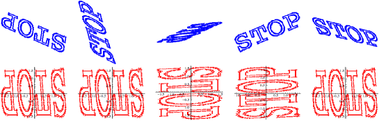
Fig. 1: Normalization by optimization over orbit generated by special linear group $\mathfrak{SL}(2)$ for 2D point clouds. The first row contains point clouds before normalization; the second row consists of corresponding point clouds after normalization for each entry in the first row. It can be observed that point clouds in the second row are approximately the same, modulo four orientations (rotated clockwise by angle of 0, $\frac{\pi}{2}$, $\pi$, $\frac{3\pi}{2}$).

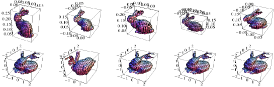
Fig. 2: Normalization by optimization over orbit generated by special linear group $\mathfrak{SL}(3)$ for 3D point clouds. The first row contains point clouds before normalization. In particular, the “rabbits” are of different shapes and sizes. The second row consists of corresponding point clouds after normalization for each entry in the first row. It can be observed that point clouds in the second row are approximately the same, modulo different orientations of the same shape.

In this paper we study the cases when degrees of freedom to be removed have a group structure ${\mathfrak{G}}$ when combined. Under such a condition, a data matrix ${\bf X}$ can be mapped to its quotient set ${\bf X}/\sim$ by the equivalence relation $\sim$ defined as

$$x_{1}\sim x_{2}\iff\exists g\in{\mathfrak{G}},x_{1}=gx_{2}\text{.}$$

We call the elements of quotient set $\hat{{\bf X}}\in{\bf X}/\sim$ canonical forms of data, as they are invariant with respect to (w.r.t.) group actions $g\in{\mathfrak{G}}$. An important example of using the quotient set is the shape space method [4], which works in the quotient space of rotation matrix and is closely related to PCA and SVD.

Here and later, we restrict ourselves to the case when ${\mathfrak{G}}$ is a matrix group and when the group acts by simple matrix product. The quotient mapping ${\bf X}\rightarrow\hat{{\bf X}}$ can then be represented in the form of matrix decomposition:

$${\bf X}={\bf G}\hat{{\bf X}}\text{, }{\bf G}\in{\mathfrak{G}}\text{.}$$

Instead of constructing separate algorithms for different ${\mathfrak{G}}$, we use an optimization process to induce corresponding matrix decomposition techniques. In particular, given a data matrix ${\bf M}$, we consider a group orbit optimization (GOO) problem as follows:

(1) $$\inf_{{\bf G}\in{\mathfrak{G}}}\;\phi({\bf G}{\bf M}),$$

where $\phi:{\mathbb{F}}^{n_{1}\times n_{2}}\rightarrow{\mathbb{R}}$ is a cost function and ${\mathbb{F}}$ is some number field.

In Section 3 we present several special classes of cost functions, which are used to construct new formulations for several matrix decompositions including SVD, Schur, LU, Cholesky and QR in Section 4. As an application, in Section 6 we illustrate how to use GOO to normalize low dimensional point cloud data over a special linear group. Experiment results for two-dimensional and three-dimensional point cloud are given in Figure 1 and Figure 2. It can be observed that the effect of rotation, shearing and squeezing in data has been mostly eliminated in the normalized point clouds. The detail of this normalization is explained in Section 6.

The GOO formulation also allows us to construct generalizations of some matrix decompositions to tensor. Real world data have tensor structure when some value depends on multiple factors. For example, in an electronic-commerce site, user preferences in different brands form a matrix. As such preferences change over time, the time-dependent preferences form a 3 order tensor. As in the matrix case, tensor decomposition techniques [13, 14] aim to eliminate degrees of freedom in data while respecting the tensor structure of data. In Section 5, we use GOO to induce tensor decompositions that can be used for normalizing tensor. In the unified framework of GOO, the GOO inducing tensor decomposition when applied to a 2 order tensor, is exactly the same as the GOO inducing matrix decomposition, when the same group and cost function is used for both GOO problems.

The remainder of paper is organized as follows. Section 2 gives notation used in this paper. Section 3 defines several properties for describing the cost function used in defining GOO to induce matrix and tensor decompositions. Section 4 studies GOO formulations that can induce SVD, Schur, LU, Cholesky, QR, etc. Section 5 demonstrates how to use GOO to induce tensor decompositions and prove a few inequalities relating a few forms of GOO. Section 6 demonstrates how to normalize point cloud data distorted by rotation, shearing and squeezing with GOO over the special linear group. Section 7 presents numerical algorithms and examples of matrix decomposition, point cloud normalization and tensor decomposition. Finally, we conclude the work in Section 9.

2 Notation

2.1 Matrix operation notation

In this paper, we let ${\bf I}_{r}$ denote the $r\times r$ identity matrix. Given an $n{\times}m$ matrix ${\bf X}=[x_{ij}]$, we denote $|{\bf X}|=[|x_{ij}|]$ and $\operatorname{vec}({\bf X})=[x_{11},\ldots,x_{n1},x_{12},\ldots,x_{nm}]^{\top}$. The $\ell_{p}$-norm of ${\bf X}$ is defined by

$$\|{\bf X}\|_{p}\overset{\mathrm{def}}{=\joinrel=}(\sum_{ij}|x_{ij}|^{p})^{\frac{1}{p}}$$

for $p\geq 0$. Note that we abuse the notation a little bit as $\|{\bf X}\|_{p}$ is not a norm when $p<1$. When $p=2$, it is also called the Frobenius norm and usually denoted by $\|{\bf X}\|_{F}$. When applied to vector ${\bf x}$, $\|{\bf x}\|_{2}$ is the $\ell_{2}$-norm and it is shortened as $\|{\bf x}\|$. The dual norm of the $p$-norm where $p\geq 1$ is equivalent to the $q$-norm, where $\frac{1}{p}+\frac{1}{q}=1$. We let $\|{\bf X}\|_{*p}$ denote the Schatten $p$-norm; that is, it is the $\ell_{p}$ norm of the vector of the singular values of ${\bf X}$.

Assume that $\mathbb{F}$ is some number field. Let ${\bf X}^{\mathrm{c}}$ be the complex conjugate of ${\bf X}$, and ${\bf X}^{*}$ be the complex conjugate transpose of ${\bf X}$. Let $\operatorname{dg}({\bf M})$ be a vector consisting of the diagonal entries of ${\bf M}$, and $\operatorname{diag}({\bf v})$ be a matrix with ${\bf v}$ as its diagonals.

Given two matrices ${\bf A}$ and ${\bf B}$, ${\bf A}\odot{\bf B}$ is their Hadamard product and ${\bf A}\otimes{\bf B}$ is the Kronecker product. Similarly, ${\bf x}\otimes{\bf y}$ is the Kronecker product of vectors ${\bf x}$ and ${\bf y}$. For groups ${\mathfrak{G}}_{1}$ and ${\mathfrak{G}}_{2}$, we denote group $\{{\bf G}_{1}\otimes{\bf G}_{2}:\,{\bf G}_{1}\in{\mathfrak{G}}_{1},{\bf G}_{2}\in{\mathfrak{G}}_{2}\}$ as ${\mathfrak{G}}_{1}\otimes{\mathfrak{G}}_{2}$. The Kronecker sum for two square matrices ${\bf A}\in{\mathbb{F}}^{m\times m},{\bf B}\in{\mathbb{F}}^{n\times n}$ is defined as

$${\bf A}\oplus{\bf B}={\bf A}\otimes{\bf I}_{n}+{\bf I}_{m}\otimes{\bf B}\text{.}$$

Definition 1.

A matrix ${\bf A}\in\mathbb{F}^{m\times n}$ is said to be pseudo-diagonal if there exist permutation matrices ${\bf P}$ and ${\bf Q}$ such that ${\bf P}{\bf A}{\bf Q}^{\top}$ is diagonal.

Remark 2.

Note that a diagonal matrix is also pseudo-diagonal.

Lemma 3.

Given a pseudo-diagonal matrix ${\bf A}$, we have that

1. ${\bf A}^{*}{\bf A}$, ${\bf A}{\bf A}^{*}$, ${\bf A}^{\top}{\bf A}$ and ${\bf A}{\bf A}^{\top}$ are diagonal.

2. There exists a row permutation matrix ${\bf P}$ such that ${\bf P}{\bf A}$ is diagonal.

3. There exists a row permutation matrix ${\bf P}$ such that ${\bf A}{\bf P}^{\top}$ is diagonal.

We let $\operatorname{Poly}{({\bf M})}$ be the polyhedral formed by points with coordinates being rows of ${\bf M}$, and $\mu(\operatorname{Poly}{({\bf M})})$ be the Lebesgue measure of $\operatorname{Poly}{({\bf M})}$. We let $\operatorname{Rasterize}(\operatorname{Poly}{({\bf M})})$ be a matrix ${\bf Z}$ where $z_{ij}$ is the image pixel value at coordinate $(i,j)$ of image rasterized from polyhedral $\operatorname{Poly}{({\bf M})}$ with unit grid.

2.2 Tensor operation notation

The notation of tensor operations used in this paper mostly follows that of [13]. Given an order-$k$ tensor ${\mathcal{X}}\in\mathbb{F}^{n_{1}\times n_{2}\times\ldots\times n_{k}}$ and $k$ matrices $\{{\bf U}_{i}\}_{i=1}^{k}$ where ${\bf U}_{i}\in\mathbb{F}^{m_{i}\times n_{i}}$, we define $\times_{k}$ to be the inner product over the $k$-th mode. That is, if ${\mathcal{Y}}={\mathcal{X}}\times_{a}{\bf U}_{a}\in\mathbb{F}^{n_{1}\times n_{2}\times\ldots\times n_{a-1}\times m_{a}\times n_{a+1}\times\ldots\times n_{k}}$, then

$$y_{i_{1}\cdots i_{a-1}ji_{a+1}\cdots i_{k}}=\sum_{i_{a}=1}^{n_{a}}x_{i_{1}i_{2}\cdots i_{k}}u_{ji_{a}}.$$

For shorthand, we denote

$$\prod_{i}{\mathcal{X}}{\bf U}_{i}\overset{\mathrm{def}}{=\joinrel=}{\mathcal{X}}\times_{1}{\bf U}_{1}\times_{2}{\bf U}_{2}\cdots\times_{k}{\bf U}_{k}\textrm{.}$$

Here ${\mathcal{Y}}=\prod_{i}{\mathcal{X}}{\bf U}_{i}$ when $\forall i,m_{i}=n_{i}$ is also known as the Tucker decomposition in the literature [24]. With this notation, the SVD of a real matrix ${\bf M}={\bf U}_{1}\mbox{\boldmath$\Sigma$\unboldmath}{\bf U}_{2}^{\top}$ can be written as

$${\bf M}=\mbox{\boldmath$\Sigma$\unboldmath}\times_{1}{\bf U}_{1}\times_{2}{\bf U}_{2}=\prod_{i=1}^{2}\mbox{\boldmath$\Sigma$\unboldmath}{\bf U}_{i}\text{.}$$

Using the vectorization operation for tensor, we have

$$\operatorname{vec}{(\prod_{i}{\mathcal{X}}{\bf U}_{i})}=[{\bf U}_{n}\otimes{\bf U}_{n-1}\otimes\dotsb\otimes{\bf U}_{1}]\operatorname{vec}{({\mathcal{X}})}\overset{\mathrm{def}}{=\joinrel=}\otimes^{\downarrow}_{i}{\bf U}_{i}\operatorname{vec}{({\mathcal{X}})},$$

where we denote $\otimes^{\downarrow}_{i}{\bf U}_{i}$ as shorthand for ${\bf U}_{n}\otimes{\bf U}_{n-1}\otimes\dotsb\otimes{\bf U}_{1}$.

We let $\operatorname{index}_{n_{1},n_{2},\ldots,n_{k}}(I)$ be a map from a sequence of indices $I={i_{1},i_{2},\ldots,i_{k}}$ to an integer such that

(2) $$[\operatorname{vec}{{\mathcal{X}}}]_{\operatorname{index}_{n_{1},n_{2},\ldots,n_{k}}({i_{1},i_{2},\ldots,i_{k}})}={\mathcal{X}}_{i_{1},i_{2},\ldots,i_{k}}\textrm{.}$$

We note that $\operatorname{index}^{-1}_{N}(n)$ is well-defined.

The unfold operation maps a tensor to a tensor of lower order and is defined by

$$\operatorname{fold}^{-1}_{J}:{\mathbb{F}}^{n_{1}\times n_{2}\times\ldots\times n_{k}}\mapsto\mathbb{F}^{m_{1}\times m_{2}\times\ldots\times m_{l}}\;,$$

where $J$ is an index set grouping of the indices $I=\{1,2,\ldots,k\}$ into sets $J=\{J_{1},J_{2},\ldots,J_{l}\}$, $m_{o}=\prod_{t\in J_{o}}t$, and satisfies:

$$\operatorname{vec}[\operatorname{fold}^{-1}_{J}({\mathcal{A}})]=\operatorname{vec}({\mathcal{A}})\text{.}$$

When unfolding a single index, i.e., $J=\{\{j\},I-\{j\}\}$, we also denote $\operatorname{fold}^{-1}_{J}$ as $\operatorname{fold}^{-1}_{j}$.

The $\ell_{p}$-norm of tensor ${\mathcal{A}}$ is defined as

$$\|{\mathcal{A}}\|_{p}\overset{\mathrm{def}}{=\joinrel=}\|\operatorname{fold}^{-1}_{i}\mathcal{A}\|_{p}$$

for an arbitrary mode $i$. For tensors ${\mathcal{A}},{\mathcal{B}}\in{\mathbb{F}}^{n_{1}\times n_{2}\times\ldots\times n_{k}}$, $\langle{\mathcal{A}},{\mathcal{B}}\rangle$ is their Frobenius inner product defined as:

$$\langle{\mathcal{A}},{\mathcal{B}}\rangle\overset{\mathrm{def}}{=\joinrel=}\langle\operatorname{vec}({\mathcal{A}}),\operatorname{vec}({\mathcal{B}})\rangle\text{.}$$

Finally, given $f:{\mathbb{F}}\rightarrow{\mathbb{F}}$ and ${\mathcal{T}}\in{\mathbb{F}}^{n_{1}\times n_{2}\times\ldots\times n_{k}}$, $f({\mathcal{T}})$ is defined as a tensor-valued function with $f$ applied to each entry of ${\mathcal{T}}$. Therefore, $f({\mathcal{T}})\in{\mathbb{F}}^{n_{1}\times n_{2}\times\ldots\times n_{k}}$. When $f(x)=|x|$, we denote $f({\mathcal{T}})$ as $|{\mathcal{T}}|$.

2.3 Group notation

$\mathfrak{O}$ is the orthogonal group over real field ${\mathbb{R}}$. $\mathfrak{SO}$ is the special orthogonal group over ${\mathbb{R}}$. $\mathfrak{U}$ is the unitary group over complex field. We let $\mathfrak{UUT}(n)$ denote the upper-unit-triangular group and $\mathfrak{LUT}(n)$ denote the lower-unit-triangular group, both of which have all entries along the diagonals being $1$. $\mathfrak{H}$ is the group formed by (calibrated) homography transform below:

$${\bf H}_{2w}={\bf R}_{2w}({\bf I}_{3}+{\bf p}_{2}\frac{{\bf n}^{\top}}{d})\text{,}$$

where ${\bf R}_{2w}\in\mathfrak{SO}$ is attitude of the camera; ${\bf p}_{2}$ is position of the camera, and ${\bf n}^{\top}{\bf x}=d$ is equation of the object plane.

3 Preliminaries

In this paper we would like to show that matrix and tensor decompositions techniques can be induced from formulations of the group orbit optimization. As we have seen in formula (1), a GOO problem includes two key ingredients: a cost function $\phi$ and a group structure ${\mathfrak{G}}$. Thus, we present preliminaries, including sparsifying function and a unit matrix group. The sparsifying functions will be used to define cost functions for some matrix decompositions in Table 1 that have diagonal matrices in decomposed formulations.

It should be noted that other classes of functions can be used together with some unit matrix groups to induce interesting matrix and tensor decompositions. Confer Schur decomposition in Table 1 for an example.

3.1 Sparsifying functions

For two functions $f$ and $g$, we here and later denote their composition as $f\circ g$ s.t. $f\circ g(x)\overset{\mathrm{def}}{=\joinrel=}f(g(x))$. We first prove several utility lemmas used for characterizing sparsifying functions.

Lemma 4 (Subadditive properties).

If $f(\sqrt{x})$ is subadditive, then

1. $\sum_{i=1}^{n}f(|x_{i}|)\geq f(\|{\bf x}\|)$ where ${\bf x}\in{\mathbb{F}}^{n}$.

2. $f(0)\geq 0$.

Proof.

First we have that $\sum_{i=1}^{n}f(|x_{i}|)=\sum_{i=1}^{n}f(\sqrt{x_{i}^{2}})\geq f(\sqrt{\sum_{i=1}^{n}x_{i}^{2}})=f(\|{\bf x}\|)$. By the subadditivity of $f(\sqrt{x})$ we further have $f(\sqrt{0})+f(\sqrt{0})\geq f(\sqrt{0+0})=f(\sqrt{0})$, hence $f(0)=f(\sqrt{0})\geq 0$. ∎

Lemma 5.

If $f(e^{x})$ is convex for any $x\in{\mathbb{F}}$, then when $\forall i,x_{i}\neq 0$, we have:

$$\sum_{i=1}^{n}f(|x_{i}|)\geq nf\big{(}(\prod_{i=1}^{n}|x_{i}|)^{\frac{1}{n}}\big{)}\quad.$$

Proof.

Since $f(e^{x})$ is convex, we have

$$\sum_{i=1}^{n}f(|x_{i}|)=\sum_{i=1}^{n}f(e^{\ln|x_{i}|})\geq nf(e^{\frac{1}{n}\sum_{i=1}^{n}\ln|x_{i}|})=nf((\prod_{i=1}^{n}|x_{i}|)^{\frac{1}{n}}).$$

∎

Lemma 6.

If $f$ is strictly concave and $f(0)\geq 0$, then $f(tx)\geq tf(x)$ where $0\leq t\leq 1$, with equality only when $t=0,1$ or $x=0$.

Proof.

We have $f(tx)=f(tx+(1-t)0)\geq tf(x)+(1-t)f(0)\geq tf(x)$. Obviously, the first equality holds only when $x=0$ or $t=0,1$. ∎

Lemma 7.

Assume $f(x)=f(|x|)$. Then $f$ is concave and $f(0)\geq 0$ iff $f$ is concave and subadditive.

Proof.

Because $f(x)=f(|x|)$, w.l.o.g. we assume $x\geq 0$. We first prove “$\Rightarrow$ part”. When $a=0$ and $b=0$, we trivially have $f(a)+f(b)\geq f(a+b)$. Otherwise, we have

$$f(tx)=f(tx+(1-t)0)\geq tf(x)+(1-t)f(0)\geq tf(x)\text{.}$$

Thus, when $a\neq 0$ or $b\neq 0$,

$$f(a)+f(b)=f(\frac{(a+b)a}{a+b})+f(\frac{(a+b)b}{a+b})\geq\frac{a}{a+b}f(a+b)+\frac{b}{a+b}f(a+b)=f(a+b)\text{.}$$

As for “$\Leftarrow$ part”, we have $f(0)+f(0)\geq f(0+0)$. Hence $f(0)\geq 0$. ∎

Now we are ready to define the sparsifying function.

Definition 8 (sparsifying function).

A function f is sparsifying if

1. $f$ is symmetric about the origin; i.e., $f(x)=f(|x|)$;

2. $f(\sum_{i}|x_{i}|)=\sum_{i}f(|x_{i}|)\Longrightarrow$ there is at most one $i$ with $x_{i}\neq 0$.

The following theorem gives a sufficient condition for function $f$ to be sparsifying.

Theorem 9 (sufficient condition for sparsifying).

If $f(x)=f(|x|)$ and $f$ is strictly concave and subadditive, then $f$ is sparsifying.

Proof.

Because $f(x)=f(|x|)$, w.l.o.g. we assume $x\geq 0$. By Lemma 7, $f$ is strictly concave and $f(0)\geq 0$. When $\sum_{i}x_{i}=0$, there is no $i$ with $x_{i}=0$. Otherwise, it follows from Lemma 6 that

$$\sum_{i}f(x_{i})=\sum_{i}f\big{(}\frac{x_{i}}{\sum_{j}x_{j}}\sum_{j}x_{j}\big{)}\geq\sum_{i}\frac{x_{i}}{\sum_{j}x_{j}}f(\sum_{j}x_{j})=f(\sum_{j}x_{j})\text{.}$$

Also by Lemma 6, the equality holds iff $\frac{x_{i}}{\sum_{j}x_{j}}=0\text{ or }1$. Because $\sum_{i}\frac{x_{i}}{\sum_{j}x_{j}}=1$, there is only one $i$ with $x_{i}\neq 0$. In both cases, there is at most one $i$ with $x_{i}\neq 0$. ∎

Corollary 10.

Conical combination of sparsifying functions. In particular, if $f$ and $g$ are sparsifying, then so is $\alpha f+\beta g$ where $\alpha$ and $\beta$ are two nonnegative constants.

Proof.

As strict concavity is preserved by conical combination, we only need prove subadditivity is preserved by conical combination, which holds because:

$$(\alpha f+\beta g)(x+y) =\alpha f(x+y)+\beta g(x+y)$$

$$\leq\alpha f(x)+\alpha f(y)+\beta g(x)+\beta g(y)$$

$$=(\alpha f+\beta g)(x)+(\alpha f+\beta g)(y).$$

∎

It can be directly checked that the following functions are sparsifying.

Example 11.

Following functions are sparsifying:

1. Power function: $f(x)=|x|^{p}$ for $0<p<1$;

2. Capped power function: $f(x)=\min(|x|^{p},1)$ for $0<p<1$;

3. $f(x)=-|x|^{p}$ for $p>1$;

4. $f(x)=\log(1+|x|)$;

5. Shannon Entropy: $f(x)=-|x|\log|x|$ when $0\leq x$;

6. Squared entropy: $f(x)=-x^{2}\log x^{2}$ when $0\leq x$;

7. $f(x)=a-(a+|x|^{p})^{\frac{1}{p}}$ for $p>1$ and $a\geq 0$;

8. $f(x)=-a+(a+|x|^{p})^{\frac{1}{p}}$ for $p<1$ and $a\geq 0$;

Remark 12.

We note that $\log|x|$ is not subadditive because $f(0)=-\infty<0$. Although $f(x)=|x|^{p}$ for $p<0$ is subadditive, $|x|^{p}$ is not concave. Thus, these two functions are not sparsifying.

3.2 Unit Matrix Groups

Definition 13 (unit group).

A matrix group ${\mathfrak{G}}$ is a unit group if $|\det({\bf G})|=1,\,\forall{\bf G}\in{\mathfrak{G}}$.

Clearly, unitary, orthogonal, and unit-triangular matrix groups are unit groups. We now present some properties of the unit groups.

Lemma 14.

Unit group has the following properties.

1. Unit group is well-defined, i.e., closed under multiplication and inverse, and has an identity element which happens to be ${\bf I}$.

2. The Kronecker product of unit groups is also a unit group. In particular, if ${\mathfrak{G}}_{1}$ and ${\mathfrak{G}}_{2}$ are unit groups, then ${\mathfrak{G}}_{1}\otimes{\mathfrak{G}}_{2}=\{{\bf M}_{1}\otimes{\bf M}_{2}:{\bf M}_{1}\in{\mathfrak{G}}_{1}\mbox{ }{\bf M}_{2}\in{\mathfrak{G}}_{2}\}$ is also a unit group.

3. $\{{\bf P}\otimes{\bf P}^{-\top}:{\bf P}\in\mathfrak{GL}(n)\}$ is a unit group.

4. $\{{\bf A}\otimes{\bf A}^{\mathrm{c}}:{\bf A}\in\mathfrak{GL}(n)\}$ is a group, and is a unit group iff $\mathfrak{GL}(n)$ is a unit group.

5. $\{{\bf I}_{n}\otimes{\bf A},{\bf A}\in{\mathfrak{G}}\}$ is a unit group iff ${\mathfrak{G}}$ is a unit group. $\{{\bf A}\otimes{\bf I}_{n},{\bf A}\in{\mathfrak{G}}\}$ is a unit group iff ${\mathfrak{G}}$ is a unit group.

Proof.

1. Let ${\bf G}_{1},{\bf G}_{2}\in{\mathfrak{G}}$. Then $|\det({\bf G}_{1}^{-1})|=1$ and

   $$|\det({\bf G}_{1}{\bf G}_{2})|=|\det({\bf G}_{1})||\det({\bf G}_{2})|=1.$$

   Hence ${\bf G}_{1}^{-1}\in{\mathfrak{G}}$ and ${\bf G}_{1}{\bf G}_{2}\in{\mathfrak{G}}$.

2. We first check ${\mathfrak{G}}_{1}\otimes{\mathfrak{G}}_{2}$ is a group. This can be done by noting that $({\bf G}_{1}\otimes{\bf G}_{2})^{-1}={\bf G}_{1}^{-1}\otimes{\bf G}_{2}^{-1}\in{\mathfrak{G}}_{1}\otimes{\mathfrak{G}}_{2}$ when ${\bf G}_{1}\in{\mathfrak{G}}_{1}$, ${\bf G}_{2}\in{\mathfrak{G}}_{2}$; and

   $$({\bf G}_{1}\otimes{\bf G}_{2})({\bf G}_{3}\otimes{\bf G}_{4})=({\bf G}_{1}{\bf G}_{3})\otimes({\bf G}_{2}{\bf G}_{4})\text{.}$$

   Also ${\bf I}\in{\mathfrak{G}}_{1}\otimes{\mathfrak{G}}2$. Moreover, since $|\det({\bf G}_{1}\otimes{\bf G}_{2})|=|\det({\bf G}_{1})|^{m}|\det({\bf G}_{2})|^{n}=1$ for any ${\bf G}_{1}\in{\mathfrak{G}}_{1}$ and ${\bf G}_{2}\in{\mathfrak{G}}_{2}$, ${\mathfrak{G}}_{1}\otimes{\mathfrak{G}}_{2}$ is a unit group.

3. Closedness under multiplication and inverse can be proved by noting

   $$({\bf P}\otimes{\bf P}^{-\top})({\bf Q}\otimes{\bf Q}^{-\top})=({\bf P}{\bf Q})\otimes({\bf P}^{-\top}{\bf Q}^{-\top})=({\bf P}{\bf Q})\otimes({\bf P}{\bf Q})^{-\top}\text{.}$$

   Also we have

   $$({\bf P}\otimes{\bf P}^{-\top})^{-1}={\bf P}^{-1}\otimes{\bf P}^{\top}\text{.}$$

   Thus ${\bf P}\otimes{\bf P}^{-\top}$ forms a group with ${\bf I}$ as the identity. It is also a unit group as $|\det({\bf P}\otimes{\bf P}^{-\top})|=|\det({\bf P})^{n}\det({\bf P}^{-\top})^{n}|=1$.

4. Closedness under multiplication and inverse can be proved based on

   $$({\bf L}\otimes{\bf L}^{\mathrm{c}})({\bf R}\otimes{\bf R}^{\mathrm{c}})=({\bf L}{\bf R})\otimes({\bf L}^{\mathrm{c}}{\bf R}^{\mathrm{c}})=({\bf L}{\bf R})\otimes{\bf L}{\bf R}^{\mathrm{c}}\text{,}$$

   and $({\bf L}\otimes{\bf L}^{\mathrm{c}})^{-1}={\bf L}^{-1}\otimes({\bf L}^{-1})^{\mathrm{c}}$. Thus ${\bf L}\otimes{\bf L}^{\mathrm{c}}$ forms a group with ${\bf I}$ as the identity. Moreover $|\det({\bf L}\otimes{\bf L}^{\mathrm{c}})|=|\det({\bf L})^{n}\det({\bf L}^{\mathrm{c}})^{n}|=|\det({\bf L})|^{2n}$, i.e., ${\bf L}\otimes{\bf L}^{\mathrm{c}}$ forms a unit group iff ${\bf L}$ is from a unit group.

5. Note $\{{\bf I}_{n}\}$ is a unit group with single element. By property (ii) we can prove this property.

∎

It is worth pointing out that ${\bf P}\otimes{\bf P}^{-1}$ does not form a group in general because $({\bf P}\otimes{\bf P}^{-1})({\bf Q}\otimes{\bf Q}^{-1})=({\bf P}{\bf Q})\otimes({\bf Q}{\bf P})^{-1}\not\equiv({\bf P}{\bf Q})\otimes({\bf P}{\bf Q})^{-1}$.

Finally, in Table 1 we list matrix decompositions of ${\bf X}$ used in this paper. When referring to the Cholesky decomposition, ${\bf X}$ should be positive definite.

Table 1: Matrix decompositions

Name	Decomposition	Constraint
real SVD	${\bf X}={\bf U}{\bf D}{\bf V}^{\top}$	${\bf U},{\bf V}\in\mathfrak{O}(n)$, ${\bf D}$ is diagonal
complex SVD	${\bf X}={\bf U}{\bf D}{\bf V}^{*}$	${\bf U},{\bf V}\in\mathfrak{U}(n)$, ${\bf D}$ is diagonal
QR	${\bf X}={\bf Q}{\bf D}{\bf R}$	${\bf Q}\in\mathfrak{U}(n),{\bf R}\in\mathfrak{UUT}(n)$, ${\bf D}$ is diagonal
LU	${\bf X}={\bf L}{\bf D}{\bf U}$	${\bf L}\in\mathfrak{LUT}(n),{\bf U}\in\mathfrak{UUT}(n)$, ${\bf D}$ is diagonal
Cholesky	${\bf X}={\bf L}{\bf D}{\bf L}^{\top}$	${\bf L}\in\mathfrak{LUT}(n)$, ${\bf D}$ is diagonal
Schur	${\bf X}={\bf Q}{\bf U}{\bf Q}^{*}$	${\bf Q}\in\mathfrak{U}(n)$, ${\bf U}$ is upper triangular

4 Group Orbit Optimization

4.1 Matrix Decomposition Induced from Group Orbit Optimization

4.1.1 GOO formulation

We now illustrate how matrix decomposition can be induced from GOO. Given two groups ${\mathfrak{G}}1,{\mathfrak{G}}2$ and a data matrix ${\bf M}$, we consider the following optimization problem

(3) $$\inf_{{\bf G}_{1}\in{\mathfrak{G}}_{1},{\bf G}_{2}\in{\mathfrak{G}}_{2}}\;\phi({\bf G}_{2}{\bf M}{\bf G}_{1}^{\top}).$$

Assume that $\hat{{\bf G}_{1}}$ and $\hat{{\bf G}_{2}}$ are minimizers of the above GOO and ${\bf D}=\hat{{\bf G}}_{2}{\bf M}\hat{{\bf G}}_{1}^{\top}$, then we refer to

$${\bf M}=\hat{{\bf G}}_{2}^{-1}{\bf D}\hat{{\bf G}}_{1}^{-\top}\text{,}$$

as a matrix decomposition of ${\bf M}$ which is induced from Formula (3).

When $\phi=\varphi\circ\operatorname{vec}$, an equivalent formulation of Formula (3) is:

$$\inf_{{\bf G}_{1}\in{\mathfrak{G}}_{1},{\bf G}_{2}\in{\mathfrak{G}}_{2}}\;\phi({\bf G}_{2}{\bf M}{\bf G}_{1}^{\top})\equiv\inf_{{\bf G}\in{\mathfrak{G}}}\varphi({\bf G}\operatorname{vec}({\bf M}))\text{,}$$

where ${\bf G}={\bf G}_{1}\otimes{\bf G}_{2}\in{\mathfrak{G}}$ and ${\mathfrak{G}}\overset{\mathrm{def}}{=\joinrel=}{\mathfrak{G}}_{1}\otimes{\mathfrak{G}}_{2}$.

4.1.2 GOO over unit group

For a general matrix group ${\mathfrak{G}}$, ${\bf G}\in{\mathfrak{G}}$ implies that $|\det({\bf G})|>0$. However, group structure may not be sufficient to induce non-trivial matrix decomposition, as with some groups and cost functions the infimum will be trivially zero. For example, with general linear group $\mathfrak{GL}$ and for any matrix ${\bf M}$, we have

$$\inf_{{\bf G}\in\mathfrak{GL}}\|{\bf G}{\bf M}\|_{p}=0,$$

because $s{\bf I}\in\mathfrak{GL}$ and

$$\lim_{s\to 0}\inf_{s\in{\mathbb{R}}}\|s{\bf I}{\bf M}\|_{p}=\lim_{s\to 0}s\|{\bf M}\|_{p}=0\;.$$

Nevertheless, if we require ${\mathfrak{G}}$ to be a unit group, we have $|\det({\bf G})|=1$. Consequently, we can prevent the infimum from vanishing trivially for any $\ell_{p}$-norm. Thus, we mainly consider the case where ${\mathfrak{G}}$ is a unit group in this paper.

The following theorem shows that many matrix decompositions can be induced from the group orbit optimization.

Theorem 15.

SVD, LU, QR, Schur and Cholesky decompositions of matrix ${\bf M}\in\mathbb{F}^{m\times n}$ can be induced from GOO of the form

$$\inf_{{\bf G}_{1}\in{\mathfrak{G}}_{1},{\bf G}_{2}\in{\mathfrak{G}}_{2}}\;\phi({\bf G}_{2}{\bf M}{\bf G}_{1}^{\top})\text{,}$$

by using the corresponding unit group ${\bf G}$ and cost function $\phi$, which are given in Table 2.

Clearly, the matrix groups in Table 2 are unit groups by Lemma 14. We will prove the rest of theorem in Section 4.2 and Section 4.3.

Remark 16.

The cost function for SVD, QR and Matrix Equivalence can be $\phi({\bf X})=\|{\bf X}\|_{p},\,1\leq p<2$. And the cost function for LU, Schur and Cholesky can be $\phi({\bf X})=\sum_{ij}\|x_{ij}{\mathbb{I}}_{\{i<j\}}\|_{p},\,1\leq p<2$.

Table 2: Matrix decompositions induced from optimizations

Decomposition	Unit group ${\mathfrak{G}}={\mathfrak{G}}_{1}\otimes{\mathfrak{G}}_{2}$	Objective function $\phi({\bf X})$
real SVD: ${\bf U}{\bf D}{\bf V}^{\top}$	$\{{\bf V}\otimes{\bf U}:{\bf U},{\bf V}\in\mathfrak{O}(n)\}$	$\sum_{ij}f(|x_{ij}|)$ where $f(\sqrt{x})$ is strictly concave, $f(0)\geq 0$
complex SVD: ${\bf U}{\bf D}{\bf V}^{*}$	$\{{\bf V}^{\mathrm{c}}\otimes{\bf U}:{\bf U},{\bf V}\in\mathfrak{U}(n)\}$	$\sum_{ij}f(|x_{ij}|)$ where $f(\sqrt{x})$ is strictly concave, $f(0)\geq 0$
QR: ${\bf Q}{\bf D}{\bf R}$	$\{{\bf R}^{\top}\otimes{\bf Q}:{\bf Q}\in\mathfrak{U}(n),{\bf R}\in\mathfrak{UUT}(n)\}$	$\sum_{ij}f(|x_{ij}|)$ where $f(\sqrt{x})$ is strictly concave and increasing, $f(0)\geq 0$
Matrix Equivalence: ${\bf P}{\bf D}{\bf Q}$	$\{{\bf Q}^{\top}\otimes{\bf P}:{\bf Q},{\bf P}\in\mathfrak{SL}(n)\}$	$\sum_{ij}f(|x_{ij}|)$ where $f(0)\geq 0$, $f(\sqrt{x})$ is strictly concave and increasing; $f(\sqrt{e^{x}})$ is convex
LU: ${\bf L}{\bf D}{\bf U}$	$\{{\bf I}\otimes{\bf L}:{\bf L}\in\mathfrak{LUT}(n)\}$	$\sum_{ij}f(|x_{ij}{\mathbb{I}}_{\{i<j\}}|)$ where $f(x)\not\equiv 0$, $f(x)=0\Rightarrow x=0$, $f(x)\geq 0$
Cholesky: ${\bf L}{\bf D}{\bf L}^{\top}$	$\{{\bf I}\otimes{\bf L}:{\bf L}\in\mathfrak{LUT}(n)\}$	$\sum_{ij}f(|x_{ij}{\mathbb{I}}_{\{i<j\}}|)$ where $f(x)\not\equiv 0$, $f(x)=0\Rightarrow x=0$, $f(x)\geq 0$
Schur: ${\bf Q}{\bf U}{\bf Q}^{*}$	$\{{\bf Q}^{\mathrm{c}}\otimes{\bf Q}:{\bf Q}\in\mathfrak{U}(n)\}$	$\sum_{ij}f(|x_{ij}{\mathbb{I}}_{\{i<j\}}|)$ where $f(x)\not\equiv 0$, $f(x)=0\Rightarrow x=0$, $f(x)\geq 0$

Remark 17.

The formulation of QR decomposition exploits the fact that ${\bf M}={\bf Q}{\bf R}$ is equivalent to ${\bf M}={\bf Q}({\bf D}\tilde{{\bf R}})$ where ${\bf Q}\in\mathfrak{U}(n)$, ${\bf R}$ is upper-triangular, $\tilde{{\bf R}}\in\mathfrak{UUT}(n)$, and ${\bf D}$ is diagonal.

Remark 18.

“Matrix Equivalence” in Table 2 finds a diagonal matrix equivalent to an invertible matrix ${\bf M}$ as defined in Section 4.2.3.

Remark 19.

However, there are matrix decompositions whose formulation cannot be expressed as GOO in the same way as Table 2. For example, Polar decomposition ${\bf M}={\bf U}{\bf L}{\bf D}{\bf L}^{*}$ where ${\bf U}\in\mathfrak{U}(n)$ and ${\bf L}\in\mathfrak{LUT}(n)$, though derivable from SVD, cannot be induced from a GOO formulation of diagonalization. This is because ${\bf L}^{\mathrm{c}}\otimes{\bf U}{\bf L}$ does not form a group as it is not closed under multiplication. For another example, consider a formulation of decomposition ${\bf M}={\bf L}{\bf D}{\bf L}^{-\top}$ where ${\bf L}\in\mathfrak{LUT}(n)$ and ${\bf D}$ is diagonal. As we stated earlier, ${\bf L}\otimes{\bf L}^{-1}$ is not a group in general, so ${\bf S}={\bf L}{\bf D}{\bf L}^{-\top}$ cannot be induced from a GOO formulation of diagonalization.

Remark 20.

For matrix decomposition of the form ${\bf M}={\bf A}{\bf D}{\bf B}^{\top}$, where ${\bf A}\in\mathbb{F}^{m\times r}$ and ${\bf B}\in\mathbb{F}^{n\times r}$ with $r\leq\min(m,n)$. In this case, we can zero-pad ${\bf D}$ to $\tilde{{\bf D}}\in\mathbb{F}^{m\times n}$, and extend ${\bf A}$ and ${\bf B}$ to $\tilde{{\bf A}}\in\mathbb{F}^{m\times m}$ and $\tilde{{\bf B}}\in\mathbb{F}^{n\times n}$ which are square matrices. Accordingly, we formulate a decomposition ${\bf M}=\tilde{{\bf A}}\tilde{{\bf D}}\tilde{{\bf B}}^{\top}$ which may be induced from GOO.

We next prove a lemma that characterizes the optimum.

Lemma 21 (Criteria for infimum).

If $\phi({\bf G}{\bf D})\geq\phi({\bf D})$ for any ${\bf G}\in{\mathfrak{G}}$ and there exists ${\bf A}\in{\mathfrak{G}}$ s.t. ${\bf M}={\bf A}{\bf D}$, then

$$\inf_{{\bf G}\in{\mathfrak{G}}}\phi({\bf G}{\bf M})=\phi({\bf D}).$$

Proof.

We note that $\inf_{{\bf G}\in{\mathfrak{G}}}\phi({\bf G}{\bf M})=\inf_{{\bf G}\in{\mathfrak{G}}}\phi({\bf G}{\bf A}{\bf D})$. By the group structure, the coset $\{{\bf G}{\bf A}:{\bf G}\in{\mathfrak{G}}\}={\mathfrak{G}}$. Hence we have

$$\inf_{{\bf G}\in{\mathfrak{G}}}\phi({\bf G}{\bf M})=\inf_{{\bf G}\in{\mathfrak{G}}}\phi({\bf G}{\bf A}{\bf D})=\inf_{{\bf G}\in{\mathfrak{G}}}\phi({\bf G}{\bf D}).$$

Using the condition $\forall{\bf G}\in{\mathfrak{G}},\phi({\bf G}{\bf D})\geq\phi({\bf D})$, we have

$$\inf_{{\bf G}\in{\mathfrak{G}}}\phi({\bf G}{\bf D})\geq\inf_{{\bf G}\in{\mathfrak{G}}}\phi({\bf D})=\phi({\bf D}).$$

On the other hand, as ${\bf I}\in{\mathfrak{G}}$ we have $\phi({\bf D})=\phi({\bf I}{\bf D})\geq\inf_{{\bf G}\in{\mathfrak{G}}}\phi({\bf G}{\bf D})$. Hence

$$\phi({\bf D})=\inf_{{\bf G}\in{\mathfrak{G}}}\phi({\bf G}{\bf D})=\inf_{{\bf G}\in{\mathfrak{G}}}\phi({\bf G}{\bf M})\text{.}$$

∎

By virtue of Lemma 21, if we want to prove that matrix decomposition $\operatorname{vec}{({\bf M})}=\tilde{{\bf G}}\operatorname{vec}{({\bf D})}$ is induced by a GOO w.r.t. $\phi$ and ${\mathfrak{G}}$, we only need prove that there exists a $\tilde{\bf G}\in{\mathfrak{G}}$ s.t. $\operatorname{vec}{({\bf M})}=\tilde{{\bf G}}\operatorname{vec}{({\bf D})}$, and $\phi({\bf G}\operatorname{vec}({\bf D}))\geq\phi(\operatorname{vec}({\bf D}))$ $\forall{\bf G}\in{\mathfrak{G}}$. The equality condition will determine the uniqueness of the optimum of the optimization problem.

4.2 Matrix Diagonalization as GOO

Next we demonstrate how matrix diagonalization can be induced from GOO with proper choice of cost function and unit group.

4.2.1 Singular Value Decomposition

First we discuss SVD of a complex matrix and of a real matrix.

Lemma 22 (Cost function and group for SVD).

Let ${\bf D}=[d_{ij}]$ be pseudo-diagonal, and ${\bf U},{\bf V}\in\mathfrak{U}(n)$. Given a function $f$ such that $f(x)=f(|x|)$ and $f(\sqrt{|x|})$ is strictly concave and subadditive, and $\phi({\bf X})=\sum_{ij}f(x_{ij})$ we have

$$\phi({\bf U}{\bf D}{\bf V}^{*})\geq\phi({\bf D}),$$

with equality iff there exists a row permutation matrix ${\bf P}$ such that $|{\bf U}{\bf D}{\bf V}^{*}|=|{\bf P}{\bf D}|$.

Furthermore, if ${\bf U},{\bf V}\in\mathfrak{O}(n)$, we have

(4) $$\phi({\bf U}{\bf D}{\bf V}^{\top})\geq\phi({\bf D}),$$

with equality iff there exists a row permutation matrix ${\bf P}$ such that $|{\bf U}{\bf D}{\bf V}^{\top}|=|{\bf P}{\bf D}|$.

Proof.

First we prove the inequality. We write $g(x)=f(\sqrt{x})$ and ${\bf A}={\bf U}{\bf D}{\bf V}^{*}$. We let $g({\bf X})=[g(x_{ij})]$ be a matrix-valued function of ${\bf X}=[x_{ij}]$. As $g$ is concave and subadditive, by Lemma 4 for a vector ${\bf v}=(v_{1},\ldots,v_{n})^{\top}$, we have $\sum_{i=1}^{n}f(v_{i})\geq f(\|{\bf v}\|)=g({\bf v}^{*}{\bf v})$. Applying this to each column of ${\bf A}$, we have

(5) $$\phi({\bf A})\geq\operatorname{tr}[g({\bf A}^{*}{\bf A})]=\operatorname{tr}[g({\bf V}{\bf D}^{*}{\bf D}{\bf V}^{*})].$$

Alternatively, we can also apply the inequality to each row of ${\bf A}$ and have

(6) $$\phi({\bf A})\geq\operatorname{tr}[g({\bf A}{\bf A}^{*})]=\operatorname{tr}[g({\bf U}{\bf D}{\bf D}^{*}{\bf U}^{*})].$$

As ${\bf D}$ is pseudo-diagonal, ${\bf D}^{*}{\bf D}$ is diagonal. Because $g$ is concave and ${\bf V}{\bf V}^{*}={\bf I}$, we can apply Jensen’s inequality, obtaining

$$\operatorname{tr}(g({\bf V}{\bf D}^{*}{\bf D}{\bf V}^{*}))\geq\operatorname{tr}({\bf V}(g({\bf D}^{*}{\bf D})){\bf V}^{*}).$$

Hence altogether we have:

$$\phi({\bf A})\geq\operatorname{tr}(g({\bf V}{\bf D}^{*}{\bf D}{\bf V}^{*}))\geq\operatorname{tr}({\bf V}(g({\bf D}^{*}{\bf D})){\bf V}^{*})=\operatorname{tr}(g({\bf D}^{*}{\bf D}))=\sum_{ij}f(d_{ij})=\phi({\bf D}).$$

Next we check the equality condition. By Theorem 9, $g$ is sparsifying. For the equality condition in inequality (5) to hold, ${\bf A}$ can have at most one nonzero in each column. By the symmetry between (5) and (6), and noting $\phi({\bf A}^{\top})=\phi({\bf A})$ and $\phi({\bf D})=\phi({\bf D}^{\top})$, ${\bf A}$ can also have at most one nonzero in each row for $\phi({\bf A})=\phi({\bf D})$ to hold. Hence when the equality holds, ${\bf A}$ is pseudo-diagonal. Then there exists a permutation matrix ${\bf P}$ such that ${\bf Z}={\bf P}^{-1}|{\bf A}|={\bf P}^{-1}{\bf Q}{\bf A}$ is a diagonal matrix with elements on diagonal in descending order and are all non-negative, where ${\bf Q}$ is a diagonal matrix s.t. $|{\bf Q}|={\bf I}$. By the uniqueness of singular values of a matrix, we have ${\bf Z}=|{\bf D}|$. Hence equality in inequality4 holds when $|{\bf A}|={\bf P}|{\bf D}|=|{\bf P}{\bf D}|$.

The proof for ${\bf U},{\bf V}\in\mathfrak{O}(n)$ is similar. ∎

Note that ${\bf D}$, modulo sign and permutation, is the global minimizer for a large class of functions $f$.

After applying Lemma 21, we have the following theorem.

Theorem 23 (SVD induced from optimization).

We are given a function $f$ such that $f(x)=f(|x|)$ and $f(\sqrt{|x|})$ is strictly concave and subadditive, and $\phi({\bf X})=\sum_{ij}f(x_{ij})$. Let $\hat{{\bf U}}$ and $\hat{{\bf V}}$ be an optimal solution of the following optimization:

$$\inf_{{\bf U}\in\mathfrak{U}(n),{\bf V}\in\mathfrak{U}(n)}\phi({\bf U}^{*}{\bf M}{\bf V}).$$

Then if SVD of ${\bf M}$ is ${\bf M}={\bf U}{\bf S}{\bf V}^{*}$, there exist a permutation matrix ${\bf P}$ and a diagonal matrix ${\bf Z}$ such that ${\bf M}=\hat{{\bf U}}{\bf P}{\bf Z}\hat{{\bf V}}^{*}$ and $|{\bf Z}|={\bf S}$.

Corollary 24.

With $\phi$ as in Theorem 23, eignedecomposition of a Hermitian matrix ${\bf M}$ can be induced from

$$\inf_{{\bf U}\in\mathfrak{U}(n)}\phi({\bf U}^{*}{\bf M}{\bf U}).$$

Similarly, eignedecomposition of a real symmetric matrix ${\bf M}$ can be induced from

$$\inf_{{\bf U}\in\mathfrak{O}(n)}\phi({\bf U}^{\top}{\bf M}{\bf U}).$$

From the above optimization, we can derive several inequalities.

Corollary 25 (The Schatten $p$-norm and $\ell_{p}$-norm inequality).

The $\ell_{p}$-norm of matrix ${\bf A}$ is larger (smaller) than the Schatten $p$-norm of ${\bf A}$ when $0\leq p<2$ $(>2)$.

In particular, we have

$$\|{\bf M}\|_{p}\geq\inf_{{\bf U},{\bf V}\in\mathfrak{U}}\|{\bf U}{\bf M}{\bf V}^{*}\|_{p}=\|{\bf M}\|_{*p}\quad\text{ when }0<p<2,$$

and

$$\|{\bf M}\|_{p}\leq\sup_{{\bf U},{\bf V}\in\mathfrak{U}}\|{\bf U}{\bf M}{\bf V}^{*}\|_{p}=\|{\bf M}\|_{*p}\quad\text{ when }p>2.$$

Proof.

$f(x)=|x|^{p}$ satisfies $f(0)\geq 0$, and $f(\sqrt{|x|})$ is strictly concave when $0\leq p<2$. On the other hand, $f(x)=-|x|^{p}$ satisfies $f(0)\geq 0$ and $f(\sqrt{|x|})$ is strictly concave when $p>2$. By Theorem 23 we have

$$\inf_{{\bf U},{\bf V}\in\mathfrak{U}}\|{\bf U}{\bf M}{\bf V}^{*}\|_{p}=\|{\bf M}\|_{*p}\quad\text{ when }0<p<2,$$

and

$$\inf_{{\bf U},{\bf V}\in\mathfrak{U}}-\|{\bf U}{\bf M}{\bf V}^{*}\|_{p}=-\|{\bf M}\|_{*p}\quad\text{ when }p>2.$$

∎

Corollary 26 (Duality gap).

Given SVD of ${\bf M}$ as ${\bf M}={\bf U}{\bf D}{\bf V}^{*}$, we have

$$\|{\bf M}\|_{p}\geq\|{\bf D}\|_{p}\geq\|{\bf D}\|_{q}\geq\|{\bf M}\|_{q}$$

where $0<p<2<q$.

Proof.

Due to the non-increasing property of the $\ell_{p}$-norm w.r.t. $p$, we have $\|{\bf D}\|_{p}\geq\|{\bf D}\|_{q}$. Also by Theorem 23 we have $\|{\bf D}\|_{p}=\|{\bf M}\|_{*p}$ and $\|{\bf D}\|_{q}=\|{\bf M}\|_{*q}$. Applying Corollary 25 completes the proof. ∎

Corollary 27.

The von Neumann entropy of density matrix ${\bf M}$ is smaller than the sum of the Shannon entropies of rows (columns) of ${\bf M}$.

Proof.

By noting that $f(x)=-x\log{x}$ is strictly concave and $f(0)\geq 0$ when $x\geq 0$, and that the von Neumann entropy is entropy of diagonal matrix in SVD of ${\bf M}$, the inequality holds. ∎

4.2.2 QR Decomposition

To derive GOO for QR decomposition, we first note that QR decomposition of a matrix ${\bf M}$ can be rewritten as ${\bf M}={\bf Q}{\bf D}{\bf R}$, where ${\bf Q}\in\mathfrak{U}(n)$, ${\bf D}$ is diagonal, and ${\bf R}\in\mathfrak{UUT}(m)$.

Lemma 28 (Cost function and group for QR).

Let $f$ satisfy that $f(x)=f(|x|)$, $f(\sqrt{x})$ is concave and increasing; $f(0)\geq 0$. Let $\phi({\bf X})=\sum_{ij}f(x_{ij})$. If ${\bf Q}\in\mathfrak{U}(n)$, ${\bf R}\in\mathfrak{UUT}(n)$, and ${\bf D}$ is diagonal, then we have

$$\phi({\bf Q}{\bf D}{\bf R})\geq\phi({\bf D}),$$

with equality when  $|{\bf Q}{\bf D}{\bf R}|=|{\bf P}{\bf D}|$, where ${\bf P}$ is a row permutation matrix.

Proof.

Let $g(x)=f(\sqrt{|x|})$ and ${\bf A}={\bf Q}{\bf D}{\bf R}$, and let $g({\bf X})=[g(x_{ij})]$. First we prove the inequality. As $g(x)$ is sparsifying and increasing, we have

$$\phi({\bf A})\geq\operatorname{tr}[g({\bf A}^{*}{\bf A})]=\operatorname{tr}[g({\bf R}^{*}{\bf D}^{*}{\bf D}{\bf R})]\geq\operatorname{tr}[g({\bf D}^{*}{\bf D})]=\phi({\bf D}).$$

Next we check the equality condition. For the equality to hold in inequality $\operatorname{tr}[g({\bf R}^{*}{\bf D}^{*}{\bf D}{\bf R})]\geq\operatorname{tr}[g({\bf D}^{*}{\bf D})]$, as $g$ is increasing, ${\bf R}$ needs to be diagonal. Hence, ${\bf R}={\bf I}$. Now for the equality to hold in $\phi({\bf A})\geq\operatorname{tr}[g({\bf A}^{*}{\bf A})]$, ${\bf A}$ needs to be pseudo-diagonal. Thus, the equality holds only when $|{\bf A}|={\bf P}|{\bf D}|=|{\bf P}{\bf D}|$ where ${\bf P}$ is a row permutation matrix. ∎

Similarly, we derive the optimization inducing QR decomposition.

Theorem 29 (QR induced from optimization).

Assume that the conditions are satisfied in Lemma 28. Let $(\hat{{\bf Q}},\hat{{\bf R}})$ be optimal solution of optimization as follows

$$\inf_{{\bf Q}\in\mathfrak{U}(n),{\bf R}\in\mathfrak{UUT}(n)}\phi({\bf Q}^{-1}{\bf M}{\bf R}^{-1})\textrm{.}$$

Then ${\bf M}=\hat{{\bf Q}}{\bf Z}$ is the QR decomposition of ${\bf M}$, where ${\bf Z}=\hat{{\bf Q}}^{-1}{\bf M}$.

4.2.3 Matrix Equivalence by the Special Linear Group

An interesting question is whether we can extend the following optimization form to more general groups ${\mathfrak{G}}_{1}$ and ${\mathfrak{G}}_{2}$:

$$\inf_{{\bf U}\in{\mathfrak{G}}_{1},\;{\bf V}\in{\mathfrak{G}}_{2}}\;\phi({\bf U}{\bf M}{\bf V}).$$

It turns out that we can use the special linear group to construct a unit group, and hence, induce matrix equivalence from an optimization.

Lemma 30 (Matrix equivalence decomposition).

An invertible matrix ${\bf M}\in\mathbb{F}^{n\times n}$ can be decomposed as ${\bf M}={\bf A}{\bf D}{\bf B}$, where $\det({\bf A})=\det({\bf B})=1$, and ${\bf D}=\det({\bf M})^{1/n}{\bf I}$.

Proof.

Just let

(7) $${\bf A}=\det({\bf M})^{-1/n}{\bf M},\quad{\bf B}={\bf I}_{n},\quad{\bf D}=\det({\bf M})^{1/n}{\bf I},$$

which gives an existence proof. ∎

Lemma 31.

If $f(\sqrt{x})$ is strictly concave and increasing, and $f(\sqrt{e^{x}})$ is convex, $f(0)\geq 0$, ${\bf A},{\bf B}\in\mathfrak{SL}(n)$ and ${\bf D}=\lambda{\bf I}$, then $\phi({\bf A}{\bf D}{\bf B})\geq\phi({\bf D})$, with equality iff there exists a permutation matrix ${\bf P}$ such that $|{\bf A}{\bf D}{\bf B}|=|{\bf P}{\bf D}|$.

Proof.

We write $g(x)=f(\sqrt{x})$ for shorthand. First prove the inequality. As ${\bf D}=\lambda{\bf I}_{n}$, we have

$$\phi({\bf A}{\bf D}{\bf B})=\phi({\bf A}{\bf B}{\bf D}).$$

As $f(\sqrt{x})$ is strictly concave and $f(0)\geq 0$, we have

$$\phi({\bf A}{\bf B}{\bf D})\geq\operatorname{tr}[g({\bf A}{\bf B}{\bf D}{\bf D}^{*}{\bf B}^{*}{\bf A}^{*})]=\operatorname{tr}[g(\lambda^{2}{\bf A}{\bf B}{\bf B}^{*}{\bf A}^{*})].$$

As ${\bf A}{\bf B}{\bf B}^{*}{\bf A}^{*}$ is Hermitian, we let its LDL decomposition be ${\bf L}{\bf Z}{\bf L}^{*}$ where ${\bf L}\in\mathfrak{LUT}(n)$. Because $g$ is increasing, we have

$$\operatorname{tr}[g(\lambda^{2}{\bf L}{\bf Z}{\bf L}^{*})]\geq\operatorname{tr}[g(\lambda^{2}{\bf Z})].$$

Because $g(e^{x})$ is convex and

$$\det({\bf Z})=\det({\bf L}{\bf Z}{\bf L}^{*})=\det({\bf A}{\bf B}{\bf B}^{*}{\bf A}^{*})=1\text{,}$$

we have

$$\operatorname{tr}[g(\lambda^{2}{\bf Z})]\geq\operatorname{tr}[g(\lambda^{2}{\bf I})].$$

In summary, we have

$$\phi({\bf A}{\bf D}{\bf B})\geq\operatorname{tr}[g(\lambda^{2}{\bf I})]=\operatorname{tr}[g({\bf D}{\bf D}^{*})]=\phi({\bf D})\textrm{.}$$

Next we check the equality condition. The equality holds in

$$\operatorname{tr}[g(\lambda^{2}{\bf L}{\bf Z}{\bf L}^{*})]\geq\operatorname{tr}[g(\lambda^{2}{\bf I})]$$

iff ${\bf L}{\bf Z}{\bf L}^{*}={\bf I}$ and ${\bf A}{\bf B}{\bf D}$ is pseudo-diagonal. Hence, the equality holds iff $|{\bf A}{\bf D}{\bf B}|={\bf P}|{\bf D}|=|{\bf P}{\bf D}|$. ∎

Theorem 32 (Matrix equivalence induced from optimization).

Let $f$ satisfy that $f(x)=f(|x|)$, $f(\sqrt{x})$ is concave, $f(\sqrt{e^{x}})$ is convex and increasing, and $f(0)\geq 0$. Let $(\hat{{\bf A}},\hat{{\bf B}})$ be an optimal solution of the following optimization problem

$$\inf_{{\bf A}\in\mathfrak{SL}(n),{\bf B}\in\mathfrak{SL}(n)}\phi({\bf A}^{-1}{\bf M}{\bf B}^{-1})\textrm{.}$$

Then there exists a row permutation matrix ${\bf P}$ such that ${\bf M}=\hat{{\bf A}}({\bf P}{\bf Z})\hat{{\bf B}}$ is the matrix equivalence decomposition of ${\bf M}$ with ${\bf P}{\bf Z}=\lambda{\bf I}$, where ${\bf Z}=(\hat{{\bf A}}{\bf P})^{-1}{\bf M}\hat{{\bf B}}^{-1}$.

4.3 Matrix Triangularization as GOO

Next we demonstrate how matrix triangularization can be induced from GOO with proper choice of cost function and unit group. In fact, we can prove that any triangularization can be induced from optimization w.r.t. a masked norm.

Lemma 33.

A matrix decomposition ${\bf M}={\bf G}_{2}{\bf U}{\bf G}_{1}^{\top},{\bf G}_{1}\in{\mathfrak{G}}_{1},{\bf G}_{2}\in{\mathfrak{G}}_{2}$, where ${\bf U}$ is upper triangular and ${\mathfrak{G}}_{1}\otimes{\mathfrak{G}}_{2}$ is a unit group, can be induced from the following optimization:

(8) $$\inf_{{\bf G}_{1}\in{\mathfrak{G}}_{1},{\bf G}_{2}\in{\mathfrak{G}}_{2}}\phi({\bf G}_{2}{\bf M}{\bf G}_{1}^{\top})\textrm{.}$$

Here $\phi({\bf X})=\sum_{ij}f(|x_{ij}{\mathbb{I}}_{\{i<j\}}|)$ where $f(x)=0\Rightarrow x=0$, $f(x)\not\equiv 0$, $f(x)\geq 0$.

Proof.

We trivially have

$$\forall{\bf G},\;\phi({\bf G}_{2}{\bf U}{\bf G}_{1}^{\top})\geq 0=\phi({\bf U})\text{.}$$

By Lemma 21 and $\phi({\bf X})=0\iff{\bf X}={\bf 0}$, the decomposition can be induced from optimization. ∎

For example, the Schur decomposition can be induced from Formula 8 with $f(x)=|x|$. We will give a numerical example in Section 7.

5 Group Orbit Optimization on Tensor Data

The GOO problem on tensor ${\mathcal{T}}$ is defined as

$$\inf_{{\bf G}_{i}\in{\mathfrak{G}}_{i}}\phi(\prod_{i}{\mathcal{T}}{\bf G}_{i}).$$

When there exists function $\varphi$ s.t. $\phi({\mathcal{T}})=\varphi(\operatorname{vec}({\mathcal{T}}))$, we get a form that bears resemblance to the matrix version:

$$\inf_{{\bf G}_{i}\in{\mathfrak{G}}_{i}}\varphi(\operatorname{vec}(\prod_{i}{\mathcal{T}}{\bf G}_{i}))=\inf_{{\bf G}_{i}\in{\mathfrak{G}}_{i}}\varphi(\otimes^{\downarrow}_{i}{\bf G}_{i}\operatorname{vec}({\mathcal{T}})).$$

Similar to the matrix case in Section 4.1, we now illustrate how the Tucker decomposition can be induced from an optimization formulation. Given a group ${\mathfrak{G}}=\otimes^{\downarrow}_{i}{\mathfrak{G}}_{i}$ and ${\bf G}=\otimes^{\downarrow}_{i}{\bf G}_{i}$ and a tensor ${\mathcal{T}}$, we define the following optimization problem

$$\inf_{{\bf G}\in{\mathfrak{G}}}\;\varphi({\bf G}\operatorname{vec}({\mathcal{T}}))=\inf_{{\bf G}_{i}\in{\mathfrak{G}}_{i}}\;\varphi((\otimes^{\downarrow}_{i}{\bf G}_{i})\operatorname{vec}({\mathcal{T}}))=\inf_{{\bf G}_{i}\in{\mathfrak{G}}_{i}}\;\varphi(\operatorname{vec}(\prod_{i}{\mathcal{T}}{\bf G}_{i}))).$$

If we assume that $\hat{{\bf G}}=\otimes^{\downarrow}_{i}{\hat{{\bf G}}_{i}}=\arg\inf_{{\bf G}\in{\mathfrak{G}}}\;\varphi({\bf G}\operatorname{vec}({\mathcal{T}}))$ and ${\mathcal{Z}}=\prod_{i}{\mathcal{T}}\hat{{\bf G}}_{i}$, then ${\mathcal{M}}=\prod_{i}{\mathcal{Z}}\hat{{\bf G}}_{i}^{-1}$ can be regarded as a tensor decomposition induced from the optimization problem.

In this section, we particularly generalize the results in Sections 3 and 4 to tensors. In Lemma 34, we prove that we can use the subgroup relation to induce a partial order of the infima of GOO. We also show that GOO w.r.t. the special linear group finds the “sparsest” Tucker-like decomposition of a tensor, and prove that GOO on tensor ${\mathcal{T}}$ is “denser” than GOO on any matrix unfolded from ${\mathcal{T}}$. We also prove Theorem 43, which says that if a tensor can be decomposed into a core tensor with certain shape, then it is optimal. As a consequence, we prove that not all tensors have superdiagonal form under a GOO w.r.t. any matrix group.

5.1 Subgroup Hierarchy

First we observe the following partial order of infima of GOO induced from a subgroup relation.

Lemma 34 (Infima partial order from subgroup relation).

If ${\mathfrak{G}}_{1}$ is a subgroup of ${\mathfrak{G}}_{2}$, then for any $\phi:{\mathbb{F}}^{n_{1}\times n_{2}\times\cdots n_{k}}\rightarrow{\mathbb{R}}$:

$$\inf_{{\bf G}\in{\mathfrak{G}}_{1}}\phi({\bf G}{\bf M})\geq\inf_{{\bf G}\in{\mathfrak{G}}_{2}}\phi({\bf G}{\bf M})\textrm{.}$$

Proof.

As ${\mathfrak{G}}_{1}$ is a subgroup of ${\mathfrak{G}}_{2}$, the set of optimization variables of the left-hand side is a subset of those of the right-hand side. Hence, the inequality holds. ∎

Corollary 35.

For a matrix ${\bf M}$, we can construct an upper bound of the Schatten $p$-norm via

$$\inf_{{\bf G}\in\mathfrak{U}}\|{\bf G}{\bf M}\|_{p}\geq\|{\bf M}\|_{*p}.$$

Proof.

$$\inf_{{\bf G}\in\mathfrak{U}}\|{\bf G}{\bf M}\|_{p}=\inf_{{\bf G}\in\mathfrak{U}}\|({\bf I}\otimes{\bf G})\operatorname{vec}({\bf M})\|_{p}\geq\inf_{{\bf G}_{1},{\bf G}_{2}\in\mathfrak{U}}\|({\bf G}_{2}\otimes{\bf G}_{1})\operatorname{vec}({\bf M})\|_{p}=\|{\bf M}\|_{*p}.$$

∎

Lemma 36 (GOO w.r.t. special linear group).

The infimum of GOO w.r.t. the special linear group is the smallest among all GOO w.r.t. a unit matrix group ${\mathfrak{G}}$ and the same $\phi$ for a tensor, that is,

(9) $$\inf_{\otimes^{\downarrow}_{i}{\bf G}_{i}\in{\mathfrak{G}}}\phi(\prod_{i}{\mathcal{T}}{\bf G}_{i})\geq\inf_{{\bf G}_{i}\in\mathfrak{SL}(n_{i})}\phi(\prod_{i}{\mathcal{T}}{\bf G}_{i})\textrm{.}$$

Proof.

First we note for ${\bf A}\in\mathbb{F}^{m\times m}$, ${\bf B}\in\mathbb{F}^{n\times n}$,

$$\det({\bf A}\otimes{\bf B})^{\frac{1}{mn}}=\det({\bf A})^{\frac{1}{m}}\det({\bf A})^{\frac{1}{n}}\textrm{.}$$

Let ${\bf Z}_{i}\in\mathfrak{GL}(n_{i})$ and $\det(\otimes^{\downarrow}_{i}{\bf Z}_{i})=1$. We can find ${\bf N}_{i}\in\mathfrak{SL}(n_{i})$ such that

$${\bf N}_{i}=(\det({\bf Z}_{i}))^{-\frac{1}{n_{i}}}{\bf Z}_{i}\;.$$

Now as $\det(\otimes^{\downarrow}_{i}{\bf Z}_{i})=\det(\otimes^{\downarrow}_{i}{\bf N}_{i})=1$, we have $\otimes^{\downarrow}_{i}{\bf N}_{i}=\otimes^{\downarrow}_{i}{\bf Z}_{i}$. By Lemma 34, we have

$$\inf_{\otimes^{\downarrow}_{i}{\bf G}_{i}\in{\mathfrak{G}}}\phi(\prod_{i}{\mathcal{T}}{\bf G}_{i})\geq\inf_{{\bf Z}_{i}\in\mathfrak{GL}(n_{i}),\det(\otimes^{\downarrow}_{i}{\bf Z}_{i})=1}\phi(\prod_{i}{\mathcal{T}}{\bf Z}_{i})=\inf_{{\bf G}_{i}\in\mathfrak{SL}(n_{i})}\phi(\prod_{i}{\mathcal{T}}{\bf G}_{i})\textrm{.}$$

∎

Next we show that GOO gives a unified framework for matrix decomposition and tensor decomposition. We can rewrite decomposition in Table 2 in tensor notation as

$${\bf M}=\prod_{i}{\bf D}{\bf G}_{i}\text{,}$$

which is induced w.r.t. a cost function $\phi$ by optimization

$$\inf_{{\bf G}\in{\mathfrak{G}}_{i}}\phi(\prod_{i}{\bf M}{\bf G}_{i})\text{.}$$

Now if there exists $\varphi$ s.t. $\phi=\varphi\circ\operatorname{vec}$, we can generalize $\phi$ to tensor as

$$\tilde{\phi}({\mathcal{T}})=<{\bf 1},\,f({\mathcal{T}})>\text{,}$$

where ${\bf 1}$ is a tensor with all entries being $1$ and of the same dimension as ${\mathcal{T}}$.

This inspires us to define a tensor version of the above optimization and decomposition as below:

$${\mathcal{T}}=\prod_{i}{\mathcal{Z}}{\bf G}_{i}\text{,}$$

and

$$\inf_{{\bf G}\in{\mathfrak{G}}_{i}}\tilde{\phi}(\prod_{i}{\mathcal{T}}{\bf G}_{i})\text{.}$$

In particular, if a matrix decomposition can be induced by entry-wise cost function $\phi({\bf M})=\sum_{ij}f(m_{ij})$ w.r.t. some unit group, we can consistently generalize the matrix decompositions to tensors using cost function $\tilde{\phi}({\mathcal{T}})=<{\bf 1},f({\mathcal{T}})>$. In this case, there is an inequality relation that follows from the Lemma 34.

Lemma 37 (Lifting lemma).

We are given a tensor ${\mathcal{T}}$ and its arbitrary unfolding $\operatorname{fold}^{-1}_{I}({\mathcal{T}})$ w.r.t. an index set grouping $I$. Let $\{m_{i}\}$ and $\{n_{j}\}$ be the sizes of the square matrices before and after grouping. Then we have

$$\inf_{{\bf M}_{i}\in{\mathfrak{G}}(m_{i})}\phi(\prod_{i}{\mathcal{T}}{\bf M}_{i})\geq\inf_{{\bf N}_{j}\in{\mathfrak{G}}(n_{j})}\phi(\prod_{j}\operatorname{fold}^{-1}_{I}({\mathcal{T}}){\bf N}_{j}).$$

Proof.

We note ${\mathfrak{G}}(a)\otimes{\mathfrak{G}}(b)$ is a subgroup of ${\mathfrak{G}}(a+b)$. Hence

$$\inf_{{\bf M}_{i}\in{\mathfrak{G}}(m_{i})}\phi(\prod_{i}{\mathcal{T}}{\bf M}_{i}) =\inf_{{\bf M}_{i}\in{\mathfrak{G}}(m_{i})}\phi((\otimes^{\downarrow}_{i}{\bf M}_{i})\operatorname{vec}({\mathcal{T}}))$$

$$\geq\inf_{{\bf N}_{j}\in{\mathfrak{G}}(n_{j})}\phi((\otimes^{\downarrow}_{j}{\bf N}_{j})\operatorname{vec}({\mathcal{T}}))$$

$$=\inf_{{\bf N}_{j}\in{\mathfrak{G}}(n_{j})}\phi(\prod_{j}\operatorname{fold}^{-1}_{I}({\mathcal{T}}){\bf N}_{j}).$$

∎

5.2 An Upper Bound for Some Tensor Norms

In the literature, there are multiple generalizations of the Schatten $p$-norm to tensors. For example, the tensor unfolding trace norm [18, 22] is defined as a weighted sum of the trace norm of single index unfoldings of the tensor; namely,

(10) $$\sum_{i=1}^{k}\alpha_{i}\|\operatorname{fold}^{-1}_{i}{\mathcal{T}}\|_{*}\;,$$

where $\alpha_{i}\geq 0$ and $\sum_{i}\alpha_{i}=1$.

Another generalization as given in [21] is defined by

(11) $$(\sum_{i=1}^{k}\frac{1}{k}\|\operatorname{fold}^{-1}_{i}{\mathcal{T}}\|_{*q}^{p})^{\frac{1}{p}}\;.$$

These tensor norms are interesting as they correspond to the Schatten norm of matrix. We next study use of the Lemma 37 to construct an upper bound for the two norms.

Formula 10 and Formula 11 try to capture the tensor structure by considering all single-index unfoldings of the tensor. However, there are many unfoldings that are not single index. In general, for a $k$th-order tensor, there are $2^{k-1}-2$ possible unfoldings, as in the following example.

Example 38.

A 3 order tensor has 3 unfoldings w.r.t. the following index set grouping: $\{\{1\},\{2,3\}\},\{\{2\},\{1,3\}\},\{\{3\},\{1,2\}\}$. Here $\{\{1\},\{2,3\}\}$ means putting index 1 of the tensor in the first dimension of the unfolded matrix, and index 2 and 3 of the tensor in the second dimension of the unfolded matrix. Additionally, a 4 th-order tensor has 6 unfoldings.

It turns out the following GOO that respects the tensor structure produces an upper bound for the Schatten $p$-norm of the matrices unfolded from a tensor.

Lemma 39 (Infimum of GOO w.r.t. the unitary group).

For $0\leq p<2$, and for any index set grouping $J$, we have:

$$\inf_{{\bf G}_{i}\in\mathfrak{U}_{i}}\|\prod_{i}{\mathcal{T}}{\bf G}_{i}\|_{p}\geq\inf_{{\bf G}_{j}\in\mathfrak{U}_{j}}\|\prod_{j}(\operatorname{fold}^{-1}_{J}{\mathcal{T}}){\bf G}_{j}\|_{p}\;.$$

Similarly for $p>2$, we have:

$$\sup_{{\bf G}_{i}\in\mathfrak{U}_{i}}\|\prod_{i}{\mathcal{T}}{\bf G}_{i}\|_{p}\leq\sup_{{\bf G}_{j}\in\mathfrak{U}_{j}}\|\prod_{j}(\operatorname{fold}^{-1}_{J}{\mathcal{T}}){\bf G}_{j}\|_{p}\;.$$

Proof.

The inequalities is obtained by applying Lemma 37 to GOO w.r.t. unitary group and $f(x)=\|x\|_{p}$ when $0\leq p<2$ and $f(x)=-\|x\|_{p}$ when $p>2$. ∎

Corollary 40.

For $0\leq p<2$, we have

$$\inf_{{\bf G}_{i}\in\mathfrak{U}_{i}}\|\prod_{i}{\mathcal{T}}{\bf G}_{i}\|_{p}\geq\sum_{i=1}^{k}\alpha_{i}\|\operatorname{fold}^{-1}_{i}{\mathcal{T}}\|_{*}\;,$$

where $\alpha_{i}\geq 0$ and $\sum_{i}\alpha_{i}=1$. We also have:

$$\inf_{{\bf G}_{i}\in\mathfrak{U}_{i}}\|\prod_{i}{\mathcal{T}}{\bf G}_{i}\|_{p}\geq(\sum_{i=1}^{k}\frac{1}{k}\|\operatorname{fold}^{-1}_{i}{\mathcal{T}}\|_{*p}^{q})^{\frac{1}{q}}.$$

Proof.

By Lemma 39, we have

$$\inf_{{\bf G}_{i}\in\mathfrak{U}_{i}}\|\prod_{i}{\mathcal{T}}{\bf G}_{i}\|_{p}\geq\max_{1\leq i\leq k}\inf_{{\bf G}_{j}\in\mathfrak{U}_{j}}\|\prod_{j}(\operatorname{fold}^{-1}_{i}{\mathcal{T}}){\bf G}_{j}\|_{p}=\max_{1\leq i\leq k}\|\operatorname{fold}^{-1}_{i}{\mathcal{T}}\|_{*p}\;.$$

We prove the inequalities as the following relations hold:

$$\max_{1\leq i\leq k}\|\operatorname{fold}^{-1}_{i}{\mathcal{T}}\|_{*p}\geq\sum_{i=1}^{k}\alpha_{i}\|\operatorname{fold}^{-1}_{i}{\mathcal{T}}\|_{*}\;,$$

and

$$\max_{1\leq i\leq k}\|\operatorname{fold}^{-1}_{i}{\mathcal{T}}\|_{*p}=(\sum_{i=1}^{k}\frac{1}{k}\max_{1\leq i\leq k}\|\operatorname{fold}^{-1}_{i}{\mathcal{T}}\|_{*p}^{q})^{\frac{1}{q}}\geq(\sum_{i=1}^{k}\frac{1}{k}\|\operatorname{fold}^{-1}_{i}{\mathcal{T}}\|_{*p}^{q})^{\frac{1}{q}}\;.$$

∎

Due to the above inequality, an optimization that tries to minimize one of tensor norms defined as in Formula 10 and Formula 11 can have the tensor norm replaced by $\inf_{{\bf G}_{i}\in\mathfrak{U}_{i}}\|\prod_{i}{\mathcal{T}}{\bf G}_{i}\|_{p}$, as minimizing upper bound of a function $f$ can always minimize $f$.

5.3 Sparse Structure in Tensor

The tensor rank is defined as the minimum number of non-zero rank-1 tensors required to sum up to ${\mathcal{T}}$, which is a generalization of the matrix rank. In the Tucker decomposition ${\mathcal{T}}=\prod_{i}{\mathcal{X}}{\bf U}_{i}$, one can define the Tucker rank w.r.t. the different constraints on the ${\bf U}_{i}$. For example, for a real tensor, when the ${\bf U}_{i}$ are required to be orthogonal, the number of nonzeros in ${\mathcal{X}}$ is defined as a tensor strong orthogonal rank of ${\mathcal{T}}$ [12]. Trivially, the tensor rank is a lower bound of all the Tucker ranks.

Tensor decomposition has a large body of the literature [7] [26] [16] [15] [17] [2] [11], the interested reader may refer to [13] and the references therein.

We find that the strong orthogonal rank of tensor ${\mathcal{T}}$ is exactly the infimum of the following GOO problem

$$\operatorname{rank}_{so}{\mathcal{T}}=\inf_{{\bf G}_{i}\in\mathfrak{U}_{i}}\|\prod_{i}{\mathcal{T}}{\bf G}_{i}\|_{0}.$$

Corollary 41.

We have

$$\inf_{\det(\otimes^{\downarrow}_{i}{\bf G}_{i})=1}\|\prod_{i}{\mathcal{T}}{\bf G}_{i}\|_{0}\geq\inf_{{\bf G}_{i}\in\mathfrak{SL}(n_{i})}\|\prod_{i}{\mathcal{T}}{\bf G}_{i}\|_{0}\geq\operatorname{rank}({\mathcal{T}})\textrm{.}$$

Proof.

The first inequality directly follows from Lemma 36 by choosing $\phi=\|\cdot\|_{0}$. For the second inequality, as the problem $\inf_{{\bf G}_{i}\in{\mathfrak{G}}_{i}}\|\prod_{i}{\mathcal{T}}{\bf G}_{i}\|_{0}$ induces a tensor decomposition into $\|\prod_{i}{\mathcal{T}}\hat{{\bf G}}_{i}\|_{0}$ number of rank-1 tensors, by definition of the tensor rank we have the following inequality:

$$\inf_{{\bf G}_{i}\in{\mathfrak{G}}_{i}}\|\prod_{i}{\mathcal{T}}{\bf G}_{i}\|_{0}\geq\operatorname{rank}({\mathcal{T}}).$$

∎

When $\phi=\|\cdot\|_{0}$, Lemma 37 provides a link between the rank of the tensor ${\mathcal{T}}$ and the ranks of the matrices or the vectors unfolded from ${\mathcal{T}}$. For example, when ${\mathfrak{G}}=\mathfrak{U}$ and ${\mathcal{T}}\neq{\bf 0}$, we have

$$\inf_{{\bf G}\in\mathfrak{U}}\|{\bf G}\operatorname{vec}({\mathcal{T}})\|_{0}=1.$$

However, for the same ${\mathcal{T}}$ unfolded to a matrix $\operatorname{fold}^{-1}_{I}({\mathcal{T}})$, we have

$$\inf_{{\bf G}_{1}\in\mathfrak{U}_{1},{\bf G}_{2}\in\mathfrak{U}_{2}}\|{\bf G}_{1}\operatorname{fold}^{-1}_{I}({\mathcal{T}}){\bf G}_{2}\|_{0}=\mathop{\operator@font rank}\nolimits(\operatorname{fold}^{-1}_{I}({\mathcal{T}}))\geq 1=\inf_{{\bf G}\in\mathfrak{U}}\|{\bf G}\operatorname{vec}({\mathcal{T}})\|_{0}.$$

Also, for the strong orthogonal rank of ${\mathcal{T}}$, we have

$$\operatorname{rank}_{so}{\mathcal{T}}=\inf_{{\bf G}_{i}\in\mathfrak{U}_{i}}\|\prod_{i}{\mathcal{T}}{\bf G}_{i}\|_{0}\geq\mathop{\operator@font rank}\nolimits(\operatorname{fold}^{-1}_{I}({\mathcal{T}})).$$

Hence, intuitively, for a higher order tensor ${\mathcal{T}}$, we can only hope to find decomposition with progressively “denser” core than the matrices and the vectors unfolded from ${\mathcal{T}}$. This can be describe more formally in the following lemma.

Lemma 42 (Optimal core when unfoldable to optimal diagonal).

If a tensor ${\mathcal{T}}$ admits a decomposition ${\mathcal{T}}=\prod_{i}{\mathcal{Z}}{\bf G}_{i}$, where ${\bf G}_{i}\in{\mathfrak{G}}_{i}$, and there exists an index set grouping $J$ such that $\otimes^{\downarrow}_{i}{\mathfrak{G}}_{i}$ is a sugroup of $\otimes^{\downarrow}_{j}\tilde{{\mathfrak{G}}}_{j}$, and

$$\inf_{\otimes^{\downarrow}_{j}\tilde{{\bf G}}_{j}\in\otimes^{\downarrow}_{j}\tilde{{\mathfrak{G}}}_{j}}\varphi((\otimes^{\downarrow}_{j}\tilde{{\bf G}}_{j})\operatorname{vec}(\operatorname{fold}^{-1}_{J}({\mathcal{Z}})))=\varphi(\operatorname{vec}(\operatorname{fold}^{-1}_{J}({\mathcal{Z}}))),$$

then ${\bf Z}$ is the optimal sparse core in the following sense:

$$\varphi(\operatorname{vec}({\mathcal{Z}}))=\inf_{{\bf G}_{i}\in{\mathfrak{G}}_{i}}\varphi(\operatorname{vec}(\prod_{i}{\mathcal{T}}{\bf G}_{i}))\;.$$

Proof.

We have

$$\varphi(\operatorname{vec}({\mathcal{Z}}))\geq\inf_{{\bf G}_{i}\in{\mathfrak{G}}_{i}}\varphi((\otimes^{\downarrow}_{i}{\bf G}_{i})\operatorname{vec}({\mathcal{Z}})) \geq\inf_{\tilde{{\bf G}}_{j}\in\tilde{{\mathfrak{G}}}_{j}}\phi((\otimes^{\downarrow}_{j}\tilde{{\bf G}}_{j})\operatorname{vec}(\operatorname{fold}^{-1}_{J}({\mathcal{Z}})))$$

$$=\varphi(\operatorname{vec}(\operatorname{fold}^{-1}_{J}({\mathcal{Z}})))=\varphi(\operatorname{vec}({\mathcal{Z}})).$$

Hence,

$$\varphi(\operatorname{vec}({\mathcal{Z}})) =\inf_{{\bf G}_{i}\in{\mathfrak{G}}_{i}}\varphi((\otimes^{\downarrow}_{i}{\bf G}_{i})\operatorname{vec}({\mathcal{Z}}))$$

$$=\inf_{{\bf G}_{i}\in{\mathfrak{G}}_{i}}\varphi(\operatorname{vec}(\prod_{i}{\mathcal{Z}}{\bf G}_{i}))=\inf_{{\bf G}_{i}\in{\mathfrak{G}}_{i}}\varphi(\operatorname{vec}(\prod_{i}{\mathcal{T}}{\bf G}_{i})).$$

∎

Applying Lemmas 22, and 31 to Lemma 42, we immediately have the following theorem.

Theorem 43.

If a tensor ${\mathcal{T}}$ admits a decomposition ${\mathcal{T}}=\prod_{i}{\mathcal{Z}}{\bf G}_{i}$, and there exists an index set grouping $J$ such that $\operatorname{fold}^{-1}_{J}({\mathcal{Z}})$ is of optimal shape w.r.t. $f$ and ${\mathfrak{G}}$ in Table 3, then ${\mathcal{Z}}$ is optimal in the sense that

$$\phi({\mathcal{Z}})=\inf_{{\bf G}_{i}\in{\mathfrak{G}}_{i}}\phi(\prod_{i}{\mathcal{T}}{\bf G}_{i}).$$

Table 3: Tensor decomposition generalized from matrix decomposition in the GOO framework

Decomposition	Optimal core shape	Unit Group	Objective function
Tensor SVD	unfoldable to some pseudo-diagonal matrix	$\mathfrak{U}$	$\sum_{ij}f(|x_{ij}|)$ where $f(\sqrt{x})$ is strictly concave, $f(0)\geq 0$
Tensor Equivalence	unfoldable to $\lambda{\bf I}_{n}$	$\mathfrak{SL}$	$\sum_{ij}f(|x_{ij}|)$ where $f(\sqrt{x})$ is strictly concave and increasing; $f(\sqrt{e^{x}})$ is convex; $f(0)\geq 0$

If a tensor ${\mathcal{T}}$ admits a decomposition ${\mathcal{T}}=\prod_{i}{\mathcal{Z}}{\bf G}_{i}$, where ${\mathcal{Z}}$ is superdiagonal, i.e., $z_{i_{1},i_{2},\cdots,i_{n}}\neq 0\Rightarrow i_{1}=i_{2}=\cdots=i_{n}$, then by Theorem 43, ${\mathcal{Z}}$ is optimal under Tensor SVD as $\operatorname{fold}^{-1}_{J}({\mathcal{Z}})$ is diagonal. However, Theorem 43 covers more cases than the superdiagonal case, like the example below: For example, consider the following 4 order tensor.

Example 44 (Non-superdiagonalizable optimal tensor).

We consider

$${\mathcal{T}}\in{\mathbb{F}}^{2\times 2\times 2\times 2},\;\operatorname{vec}{({\mathcal{T}})}=[{{{{1,0},{0,1}},{{0,0},{0,0}}},{{{0,0},{0,0}},{{1,0},{0,1}}}}]^{\top}.$$

We can unfold ${\mathcal{T}}$ to ${\bf I}_{4}$ with index set grouping $\{\{1,2\},\{3,4\}\}$. Hence, ${\mathcal{T}}$ cannot be further “sparsified” by GOO w.r.t. any matrix group, even though it is not in superdiagonal form.

Corollary 45.

There exist tensors that do not have a superdiagonal core under any Tucker decomposition induced by GOO.

Proof.

The tensor ${\mathcal{T}}$ in Example 44 can be unfolded to a scaled identity matrix. Hence, by Corollary 41 we have

$$\inf_{\det(\otimes^{\downarrow}_{i}{\bf G}_{i})=1}\|\prod_{i}{\mathcal{T}}{\bf G}_{i}\|_{0}\geq\inf_{{\bf G}_{i}\in\mathfrak{SL}(n_{i})}\|\prod_{i}{\mathcal{T}}{\bf G}_{i}\|_{0}=4.$$

This means that a Tucker decomposition of ${\mathcal{T}}$ induced by a GOO will have at least four non-zero elements in the core matrix. However, the superdiagonal core can only have at most two non-zero elements. Hence, ${\mathcal{T}}$ does not have a superdiagonal core under any Tucker decomposition induced by GOO. ∎

It is known that the minimal rank tensor decomposition in the Tucker model is not unique. For example, for tensor ${\mathcal{T}}\in{\mathbb{F}}^{2\times 2\times 2}$, we have

(12) $$\operatorname{vec}({\mathcal{T}})=[{{{1,0},{0,3}},{{0,0},{0,2}}}]^{\top}\textrm{,}$$

and there exist unitary matrices ${\bf U}_{i}\in\mathfrak{U}$ so that

(13) $$\operatorname{vec}(\prod_{i}{\mathcal{T}}{\bf U}_{i})\approx[{{{3.6055,0},{0,0.8320}},{{0,0},{0,-0.5547}}}]^{\top}\textrm{.}$$

This means that GOO by $\mathfrak{U}$ w.r.t. different $f(x)=\|x\|_{p}$ may lead to different optimum values. Hence, the class of entry-wise cost functions $f(x)=\|x\|_{p},0\leq p<2$, may not be used to induce sparsity when the optimal core tensor cannot be unfolded to a diagonal matrix. In other words, in the matrix case, any $p$, $\|x\|_{p},0\leq p<2$ can be used to find the sparest core; however, for a tensor with order larger than 3, only $f(x)=\|x\|_{0}$ can be used for finding the “sparsest” core of ${\mathcal{T}}$ under GOO. In practice, this may be done by the following asymptotic formulation:

$$\inf_{{\bf G}_{i}\in\mathfrak{U}}\|\prod_{i}{\mathcal{T}}{\bf G}_{i}\|_{0}=\lim_{p\to 0}\inf_{{\bf G}_{i}\in\mathfrak{U}}\|\prod_{i}{\mathcal{T}}{\bf G}_{i}\|_{p}.$$

In Section 7 we will present several concrete examples.

6 Data Normalization

Data normalization seeks to eliminate some arbitrary degrees of freedom in data. For example, when we are concerned with shape of an object, its attitude and position in space will become irrelevant. Given a point clouds, which is a sequence of coordinates of points, we demonstrate a method to obtain a representation of point clouds that does not depend on its attitude and position in this section. We craft the method as a special case of GOO with some particular choice of group and cost function.

6.1 Shape Analysis: Matching vs. Normalization

Point cloud data arise when interest points are extracted from images. If there are $k$ points, each with a $d$-tuple coordinate, a $k\times d$ matrix can be formed to describe the object.

Given point cloud data describing an object, shape matching tries to find an object of the closest shape within a candidate set of shapes under some measure. The shape space method for shape matching works by matching two objects with known point-to-point correspondence over given group orbits. For example, if an object described by ${\bf A}$ is known to be a rotated version of another known object ${\bf B}$, we can find out parameters describing the rotation by the following optimization formulation:

$$g({\bf A},{\bf B})\overset{\mathrm{def}}{=\joinrel=}\inf_{{\bf R}\in\mathfrak{U}(d)}\|{\bf A}{\bf R}-{\bf B}\|\textrm{.}$$

If there are $n$ candidates $\{{\bf B}_{i}\}_{i=1}^{n}$, then the best matching object can be found by $\arg\min_{i}g({\bf A},{\bf B}_{i})$.

However, to make the above method work, a point correspondence procedure must be established in the first place, which means that the same row of ${\bf A}$ and ${\bf B}$ should refer to the same point. This meets difficulties in real world data applications because

1. ${\bf A}$ and ${\bf B}$ may have different numbers of rows;

2. ${\bf A}$ and ${\bf B}$ may have many rows, leading to exponential number of possible correspondence.

Here we present a method to match point cloud by using normalization to simplify matching. The first step of the method is normalizing each of objects $\{{\bf A}_{i}\}_{i=1}^{m}$ and $\{{\bf B}_{i}\}_{i=1}^{n}$ with following optimization:

$$\hat{{\bf M}}=\mathop{\rm arginf}_{{\bf R}\in\mathfrak{U}(d)}\phi({\bf M}{\bf R})\textrm{.}$$

As in Section 4.1, the above optimization leads to following decompositions:

$${\bf A}_{i}=\hat{{\bf A}}_{i}{\bf R}_{i}\text{ and }{\bf B}_{i}=\hat{{\bf B}}_{i}{\bf U}_{i}\text{,}$$

where ${\bf R}_{i},{\bf U}_{i}\in{\mathfrak{G}}_{i}$ for some group ${\mathfrak{G}}_{i}$.

The second step of the method carries out matching of objects $\{{\bf A}_{i}\}_{i=1}^{m}$ against $\{{\bf B}_{i}\}_{i=1}^{n}$ by using the normalized forms $\{\hat{{\bf A}}_{i}\}_{i=1}^{m}$ and $\{\hat{{\bf B}}_{i}\}_{i=1}^{n}$. Matching between $\{\hat{{\bf A}}_{i}\}_{i=1}^{n}$ and $\{\hat{{\bf B}}_{i}\}_{i=1}^{n}$ is expected to be simpler because less degrees of freedom remain after normalization.

A well-known data normalization method is Principal Component Analysis (PCA), which eliminates the following degrees of freedom: translation, scaling and rotation. As any rigid body movement can be expressed as combination of translation and rotation, PCA provides a method to standardize data w.r.t. the rigid body movement. However, there may be other distortions of data. Thus, we discuss using general group for normalizing point cloud data to eliminate the effect of non-rigid body transforms. An illustrative example has been shown in Figure 1 and Figure 2 in Section 1, where we see that normalized point clouds can be matched by enumerating a small number of orientation.

6.2 Normalization of Point Cloud Data by the Special Linear Group

In this section we use group ${\bf P}^{\top}\otimes{\bf I}_{m},{\bf P}\in\mathfrak{SL}(n)$ for normalization of point cloud data.

Here we assume the distortions to the point cloud data are of a few categories of degrees of freedom: including mirroring, rotation, shearing and squeezing, which we seek to eliminate using the special linear group orbit.

Lemma 46.

The special linear group can represent any combination of mirroring, rotation, shearing and squeezing operations for point cloud data.

Proof.

Every special linear matrix ${\bf M}$ can be QR decomposed as ${\bf M}={\bf Q}{\bf R}$, and ${\bf R}$ can be decomposed into ${\bf R}={\bf D}{\bf U}$ where ${\bf D}$ is diagonal and ${\bf U}\in\mathfrak{UUT}$. Accordingly, we have a decomposition ${\bf M}={\bf Q}{\bf D}{\bf U}$, where ${\bf U}$ models the shearing operation and ${\bf Q}$ models the rotation. As $\det({\bf M})=1$, $|\det{\bf D}|=|\frac{\det{\bf M}}{\det{\bf Q}\det{\bf U}}|=1$. Hence, the diagonal matrix ${\bf D}$ is the squeezing operation (optionally with the mirror operation). Hence the action of ${\bf G}\in\mathfrak{SL}$ applied to ${\bf M}$ is equivalent to the sequential application of rotation, squeezing, mirroring, and shearing. Now as the special linear group is a group, arbitrary composition of these operations can still be represented as some ${\bf G}^{\prime}\in\mathfrak{SL}$. ∎

We show that for some point clouds, the normalized form are exactly the axis-aligned hypercubes.

Lemma 47.

Given a matrix ${\bf M}\in{\mathbb{R}}^{n\times d}$, if $\operatorname{Poly}{({\bf M})}$ is an axis-aligned hypercube and $\det{{\bf G}}=1$, then

$$\|{\bf M}{\bf G}\|_{\infty}\geq\|{\bf M}\|_{\infty}.$$

Proof.

First note that as $\det{({\bf G})}=1$, given a Lebesgue measure $\mu$, we have:

$$\mu(\operatorname{Poly}{({\bf M}{\bf G})})=\mu(\operatorname{Poly}{({\bf M})})\textrm{.}$$

We can construct a bounding box $\operatorname{Poly}{({\bf Z})}$ for $\operatorname{Poly}{({\bf M}{\bf G})}$ with center at the origin and edge length $2\|{\bf M}{\bf G}\|_{\infty}$. Note that $\operatorname{Poly}{({\bf Z})}$ is also a hypercube and $\|{\bf Z}\|_{\infty}=\|{\bf M}{\bf G}\|_{\infty}$. We thus have

$$\mu(\operatorname{Poly}{({\bf Z})})\geq\mu(\operatorname{Poly}{({\bf M}{\bf G})})=\mu(\operatorname{Poly}{({\bf M})})\textrm{.}$$

Because for any axis-aligned hypercube $\operatorname{Poly}{({\bf Y})}$ we have $\mu(\operatorname{Poly}{{\bf Y}})=2^{d}\|{\bf Y}\|_{\infty}^{d}$, the following holds:

$$2^{d}\|{\bf M}{\bf G}\|_{\infty}^{d}=2^{d}\|{\bf Z}\|_{\infty}^{d}\geq 2^{d}\|{\bf M}\|_{\infty}^{d}\textrm{.}$$

∎

By Lemma 21, we can prove the following corollary.

Corollary 48.

Let ${\bf M}\in{\mathbb{R}}^{n\times k}$ be a matrix such that $\operatorname{Poly}({\bf M})$ can be transformed by ${\bf G}\in\mathfrak{SL}(k)$ into a hypercube. Then the following optimization problem attains its optimum when $\operatorname{Poly}({\bf M}\hat{{\bf G}})$ is a hypercube:

$$\inf_{{\bf G}\in\mathfrak{SL}(n)}\|{\bf M}{\bf G}\|_{\infty}$$

Remark 49.

The optimization problem in Theorem 48 is not convex. For example, in ${\mathbb{R}}^{2}$, a square can be rotated by 90 degrees, 180 degrees, and 270 degrees while still being a square. Nevertheless, the degree of freedom associated with rotation, squeezing and shearing described by the special linear group is reduced to only one of four configurations. The three other optimal $\hat{{\bf G}}$ can be enumerated when one optimal ${\bf G}$ is known.

Remark 50.

Optimality of $\inf_{{\bf G}\in\mathfrak{SL}(2)}\|{\bf M}{\bf G}\|_{\infty}$ depends on whether $\operatorname{Poly}({\bf M}{\bf G})$ is a parallelogram. In practice, we find the above method works well in normalizing general point data, especially for those arise in shape recognition. In Section 7 we will present several concrete examples.

7 Numerical Algorithm and Examples

7.1 Algorithm

Most of optimizations involved in this paper are constrained optimization problem of the following form:

(14) $$\inf_{{\bf G}\in{\mathfrak{G}}}\;\varphi({\bf G}\operatorname{vec}({\bf M}))\text{,}$$

where ${\mathfrak{G}}$ is a unit group. When ${\mathfrak{G}}$ is a Lie group, alternatively we can turn the above optimization to another constrained optimization:

$$\inf_{{\bf G}\in{\mathfrak{g}}}\;\varphi(\exp({\bf G})\operatorname{vec}({\bf M}))\text{,}$$

where $\exp({\bf G})$ is matrix exponential of matrix ${\bf G}$ and ${\mathfrak{g}}$ is the Lie algebra associated with Lie group ${\mathfrak{G}}$. This formulation may have constraints that are easier to encode in numeric software. For example, in

$$\inf_{{\bf G}_{1}\in\mathfrak{SO}(m),{\bf G}_{2}\in\mathfrak{SO}(n)}\varphi(\operatorname{vec}({\bf G}_{2}{\bf M}{\bf G}_{1}^{\top}))\text{,}$$

we have ${\mathfrak{G}}=\mathfrak{SO}(m)\otimes\mathfrak{SO}(n)$, ${\mathfrak{g}}=\{{\bf Z}_{2}\oplus{\bf Z}_{1}:{\bf Z}_{1}\in{\mathbb{F}}^{n\times n},{\bf Z}_{1}+{\bf Z}_{1}^{\top}=0,{\bf Z}_{2}\in{\mathbb{F}}^{m\times m},{\bf Z}_{2}+{\bf Z}_{2}^{\top}=0\}$. Hence, we can turn the optimization into a constrained optimization over ${\mathfrak{g}}$ as

$$\inf_{{\bf Z}\in{\mathfrak{g}}}\varphi(\exp({\bf Z})\operatorname{vec}({\bf M}))\text{.}$$

Moreover, in this particular case, we can turn the above optimization into an unconstrained optimization:

$$\inf_{{\bf G}_{1}\in{\mathbb{F}}^{n\times n},{\bf G}_{2}\in{\mathbb{F}}^{m\times m}}\varphi(\operatorname{vec}(\exp({\bf G}_{2}-{\bf G}_{2}^{\top}){\bf M}\exp({\bf G}_{1}-{\bf G}_{1}^{\top})^{\top}))\text{.}$$

In Table 4 we list a few more cases when the constrained optimization of Formula 14 can be turned into an unconstrained optimization.

Table 4: Encoding of constraints for Lie groups

Lie group	Lie algebra	Encoding of Constraint
$\mathfrak{SO}$	$\{{\bf Z}:{\bf Z}+{\bf Z}^{\top}=0\}$	${\bf Z}={\bf X}-{\bf X}^{\top}$
$\mathfrak{LUT}$	$\{{\bf Z}:\operatorname{dg}{\bf Z}={\bf 0},{\bf Z}\in\mathfrak{LUT}\}$	${\bf Z}={\bf X}\odot[{\mathbb{I}}_{i>j}]$
$\mathfrak{UUT}$	$\{{\bf Z}:\operatorname{dg}{\bf Z}={\bf 0},{\bf Z}\in\mathfrak{UUT}\}$	${\bf Z}={\bf X}\odot[{\mathbb{I}}_{i<j}]$
$\mathfrak{SL}$	$\{{\bf Z}:\operatorname{tr}{\bf Z}=0\}$	${\bf Z}={\bf X}-(\operatorname{tr}{\bf X}){\bf v}{\bf v}^{\top}$, where ${\bf v}=[1,0,0,\ldots,0]^{\top}$
${\mathfrak{G}}_{1}\otimes{\mathfrak{G}}_{2}$	${\mathfrak{g}}_{1}\oplus{\mathfrak{g}}_{2}$

The exponential mapping used for optimization over Lie groups is related to other optimization on manifold methods [25] [5] [1].

In this section all numerical optimizations are solved by Nelder-Meld heuristic global optimization algorithm [19] implemented in Mathematica™ 9.0.0, unless noted.

7.2 GOO Inducing Matrix Decomposition

We empirically illustrate several examples of GOO inducing matrix decomposition. Due to the large amount of computation required by Nelder-Meld algorithm, here we only give a few examples involving small matrices.

Example 51 (Compute SVD of a $3\times 3$ real matrix).

Given a matrix ${\bf M}$:

$${\bf M}\approx\left[\begin{array}[]{ccc}0.17658&0.517888&0.448587\\ 0.214066&0.718154&0.849892\\ 0.796042&0.197801&0.233489\end{array}\right],$$

the SVD of ${\bf M}={\bf U}\mbox{\boldmath$\Lambda$\unboldmath}{\bf V}^{\top}$ is given as

$${\bf U}\approx\left[\begin{array}[]{ccc}-0.483076&-0.175226&-0.857865\\ -0.768129&-0.385453&0.511276\\ -0.420256&0.905937&0.0516068\end{array}\right],$$

$$\mbox{\boldmath$\Lambda$\unboldmath}\approx\left[\begin{array}[]{ccc}1.43557&0.&0.\\ 0.&0.66535&0.\\ 0.&0.&0.0910448\end{array}\right],$$

$${\bf V}\approx\left[\begin{array}[]{ccc}-0.406999&0.913369&-0.0104708\\ -0.616441&-0.28311&-0.734745\\ -0.674057&-0.292586&0.678263\end{array}\right].$$

We now use the optimization problem:

$$\inf_{{\bf U},{\bf V}\in\mathfrak{SO}(3)}\|{\bf U}^{\top}{\bf M}{\bf V}\|_{1}$$

to find the SVD of ${\bf M}$. A numerical solution, produced by the heuristic global optimization, is given as

$$\hat{{\bf U}}\approx\left[\begin{array}[]{ccc}0.483076&-0.857865&-0.175227\\ 0.768129&0.511277&-0.385453\\ 0.420256&0.0516062&0.905937\end{array}\right],$$

$$\hat{{\bf U}}^{\top}{\bf M}\hat{{\bf V}}\approx\left[\begin{array}[]{ccc}9.16351\times 10^{-10}&-8.52198\times 10^{-9}&{\bf 1.43557}\\ -4.58791\times 10^{-7}&{\bf-9.10448\times 10^{-2}}&4.36886\times 10^{-9}\\ {\bf 6.6535\times 10^{-1}}&8.13893\times 10^{-8}&2.67077\times 10^{-10}\\ \end{array}\right],$$

$$\hat{{\bf V}}\approx\left[\begin{array}[]{ccc}0.913369&0.010471&0.406999\\ -0.28311&0.734745&0.616441\\ -0.292585&-0.678263&0.674057\\ \end{array}\right].$$

Note that $\hat{{\bf U}}$, $\hat{{\bf V}}$, $\hat{{\bf U}}^{\top}{\bf M}\hat{{\bf V}}$ are permuted approximations of ${\bf U}$, ${\bf V}$, $\Lambda$ modulo sign, respectively.

Example 52 (Compute QR of a $3\times 3$ matrix).

We use the same ${\bf M}$ as in Example 51. QR decomposition of ${\bf M}$ is given by ${\bf M}={\bf Q}{\bf D}{\bf R}$ where

$${\bf Q}\approx\left[\begin{array}[]{ccc}-0.20946&-0.541716&-0.814046\\ -0.253927&-0.773817&0.580283\\ -0.944271&0.328254&0.0245274\\ \end{array}\right],$$

$${\bf D}\approx\left[\begin{array}[]{ccc}-0.843023&0.&0.\\ 0.&-0.771339&0.\\ 0.&0.&0.133735\\ \end{array}\right],$$

$${\bf R}\approx\left[\begin{array}[]{ccc}1.&0.566548&0.628984\\ 0.&1.&1.0683\\ 0.&0.&1.\\ \end{array}\right].$$

We use optimization of the form

$$\inf_{{\bf Q}\in\mathfrak{SO}(3),{\bf R}\in\mathfrak{UUT}(3)}\|{\bf Q}^{\top}{\bf M}{\bf R}^{-1}\|_{1}$$

to find QR of ${\bf M}$. A numerical solution, produced by the heuristic global optimization, is given as

$$\hat{{\bf Q}}\approx\left[\begin{array}[]{ccc}0.814046&0.541716&0.20946\\ -0.580283&0.773817&0.253927\\ -0.0245274&-0.328254&0.944271\\ \end{array}\right],$$

$$\hat{{\bf Q}}^{\top}{\bf M}\hat{{\bf R}}^{-1}\approx\left[\begin{array}[]{ccc}4.65594\times 10^{-9}&-7.03107\times 10^{-9}&\bf-1.33735\times 10^{-1}\\ 2.32509\times 10^{-8}&\bf 7.71339\times 10^{-1}&6.05164\times 10^{-9}\\ \bf 8.43023\times 10^{-1}&5.62326\times 10^{-3}&3.42317\times 10^{-9}\\ \end{array}\right],$$

$$\hat{{\bf R}}\approx\left[\begin{array}[]{ccc}1&0.559878&0.621858\\ 0&1&1.0683\\ 0&0&1\\ \end{array}\right].$$

Note that $\hat{{\bf Q}}$, $\hat{{\bf Q}}^{\top}{\bf M}\hat{{\bf R}}^{-1}$, and $\hat{{\bf R}}$ are permuted approximations of ${\bf Q}$, ${\bf D}$, ${\bf R}$ modulo sign, respectively. Note although there is a significant difference between ${\bf R}$ and $\hat{{\bf R}}$ as $\|{\bf R}-\hat{{\bf R}}\|_{F}\approx 0.00976074$, the decomposition is still good approximation as we have

$$\|\hat{{\bf Q}}\hat{{\bf D}}\hat{{\bf R}}-{\bf M}\|_{F}\approx 3.01503\times 10^{-16}\text{.}$$

Example 53 (Compute matrix equivalence decomposition of a $3\times 3$ matrix).

We use the same ${\bf M}$ as in Example 51. Matrix equivalence decomposition of ${\bf M}$ is not unique. Anyway the optimal core modulo sign and permutation would be

$${\bf D}\approx\left[\begin{array}[]{ccc}0.44304&0.&0.\\ 0.&0.44304&0.\\ 0.&0.&0.44304\end{array}\right].$$

We use the optimization

$$\inf_{{\bf A}\in\mathfrak{SL}(3),{\bf B}\in\mathfrak{SL}(3)}\|{\bf A}^{-1}{\bf M}{\bf B}^{-1}\|_{1}$$

to find the matrix equivalence decomposition of ${\bf M}$. A numerical solution produced by the heuristic global optimization is given as

$$\hat{{\bf A}}^{-1}{\bf M}\hat{{\bf B}}^{-1}\approx\left[\begin{array}[]{ccc}2.00925\times 10^{-9}&{\bf 4.42891\times 10^{-1}}&2.77141\times 10^{-9}\\ 1.18223\times 10^{-9}&2.10486\times 10^{-8}&{\bf 4.43117\times 10^{-1}}\\ {\bf 4.43112\times 10^{-1}}&-7.24341\times 10^{-9}&1.79685\times 10^{-10}\\ \end{array}\right].$$

Example 54 (Compute LU of a $3\times 3$ matrix).

We use the same ${\bf M}$ as in Example 51. The LU decomposition of ${\bf M}$ without pivoting is given by

$${\bf L}\approx\left[\begin{array}[]{ccc}1&0&0\\ 1.21229&1&0\\ 4.50812&-2.36585\times 10^{1}&1\\ \end{array}\right],$$

$${\bf U}\approx\left[\begin{array}[]{ccc}1.7658\times 10^{-1}&5.17888\times 10^{-1}&4.48587\times 10^{-1}\\ 2.77556\times 10^{-17}&9.03226\times 10^{-2}&3.06073\times 10^{-1}\\ 1.11022\times 10^{-16}&0.&5.45245\\ \end{array}\right]\textrm{.}$$

We use the optimization

$$\inf_{{\bf L}\in\mathfrak{LUT}(3)}\|\Delta\odot({\bf L}^{-1}{\bf M})\|_{1}$$

to find the LU of ${\bf M}$, where $\Delta_{ij}={\mathbb{I}}_{i>j}$. A numerical solution produced by the heuristic global optimization is given as

$$\hat{{\bf L}}\approx\left[\begin{array}[]{ccc}1&0&0\\ 1.21229&1&0\\ 4.50812&-2.36585\times 10^{1}&1\\ \end{array}\right]\textrm{,}$$

$$\hat{{\bf U}}\approx\left[\begin{array}[]{ccc}1.7658\times 10^{-1}&5.17888\times 10^{-1}&4.48587\times 10^{-1}\\ -1.64336\times 10^{-17}&9.03226\times 10^{-2}&3.06073\times 10^{-1}\\ 2.22045\times 10^{-16}&4.44089\times 10^{-16}&5.45245\\ \end{array}\right]\textrm{.}$$

Example 55 (Compute Cholesky decomposition of a $3\times 3$ matrix).

We use the ${\bf M}^{\top}{\bf M}$ as input with ${\bf M}$ from Example 51. The Cholesky decomposition of ${\bf M}^{\top}{\bf M}$ is given by ${\bf M}^{\top}{\bf M}={\bf U}^{*}{\bf U}$ where

$${\bf U}^{*}\approx\left[\begin{array}[]{ccc}0.843023&0.&0.\\ 0.477613&0.771339&0.\\ 0.530248&0.824024&0.133735\\ \end{array}\right]\textrm{.}$$

We use the optimization

$$\inf_{{\bf L}\in\mathfrak{LUT}(3)}\|\Delta\odot({\bf L}^{-1}{\bf M})\|_{1}$$

to find the LU of ${\bf M}$, where $\Delta_{ij}={\mathbb{I}}_{i>j}$. A numerical solution is given as

$$\hat{{\bf L}}\boldsymbol{\Lambda}\approx\left[\begin{array}[]{ccc}0.843023&0.&0.\\ 0.477613&0.771339&0.\\ 0.530248&0.824024&0.133735\\ \end{array}\right].$$

Here $\boldsymbol{\Lambda}$ is a diagonal matrix with square root of diagonals of $\hat{{\bf L}}^{-1}{\bf M}$ as its diagonals.

Example 56 (Compute Schur decomposition of a $3\times 3$ matrix).

We use the same ${\bf M}$ as in Example 51. The Schur decomposition of ${\bf M}={\bf Q}{\bf U}{\bf Q}^{-1}$ is given by

$$\Re{\bf Q}\approx\left[\begin{array}[]{ccc}-4.4809\times 10^{-1}&2.13496\times 10^{-2}&-3.11518\times 10^{-1}\\ -6.81147\times 10^{-1}&-5.00762\times 10^{-1}&1.85125\times 10^{-3}\\ -4.25133\times 10^{-1}&7.79816\times 10^{-1}&3.25373\times 10^{-1}\\ \end{array}\right]\textrm{,}$$

$$\Im{\bf Q}\approx\left[\begin{array}[]{ccc}-1.91558\times 10^{-1}&2.76329\times 10^{-1}&-7.67245\times 10^{-1}\\ -2.91189\times 10^{-1}&-2.4227\times 10^{-2}&4.47096\times 10^{-1}\\ -1.81744\times 10^{-1}&-2.52434\times 10^{-1}&9.23392\times 10^{-2}\\ \end{array}\right]\textrm{,}$$

$$\Re{\bf U}\approx\left[\begin{array}[]{ccc}1.38943&-2.5768\times 10^{-1}&-1.15903\times 10^{-1}\\ 0.&-1.30605\times 10^{-1}&-7.89372\times 10^{-2}\\ 0.&0.&-1.30605\times 10^{-1}\end{array}\right]\textrm{,}$$

$$\Im{\bf U}\approx\left[\begin{array}[]{ccc}-1.38778\times 10^{-16}&2.11604\times 10^{-1}&3.88987\times 10^{-2}\\ 0.&2.13379\times 10^{-1}&-5.69018\times 10^{-1}\\ 0.&0.&-2.13379\times 10^{-1}\\ \end{array}\right]\textrm{,}$$

We can use the optimization

$$\inf_{{\bf Q}\in\mathfrak{U}(3)}\|\Delta\odot({\bf Q}^{-1}{\bf M}{\bf Q})\|_{1}$$

to find the Schur decomposition of ${\bf M}$, where $\Delta_{ij}={\mathbb{I}}_{i>j}$. A numerical solution is given as

$$\Re\hat{{\bf Q}}\approx\left[\begin{array}[]{ccc}-0.159122&0.456745&-0.924103\\ -0.697698&0.596808&0.46622\\ 0.777452&0.665151&0.227028\end{array}\right]\textrm{,}$$

$$\Im\hat{{\bf Q}}\approx\left[\begin{array}[]{ccc}-0.288006&-0.0686255&0.0156732\\ 0.161731&0.0500731&0.177932\\ 0.0861939&0.00219548&-0.301602\end{array}\right]\textrm{,}$$

$$\Re\hat{{\bf U}}\approx\left[\begin{array}[]{ccc}\bf-1.30605\times 10^{-1}&-3.71633\times 10^{-1}&-7.07291\times 10^{-1}\\ -2.09852\times 10^{-9}&\bf 1.38943&-1.09975\times 10^{-1}\\ -1.39859\times 10^{-8}&9.97677\times 10^{-9}&\bf-1.30604\times 10^{-1}\end{array}\right]\textrm{,}$$

$$\Im\hat{{\bf U}}\approx\left[\begin{array}[]{ccc}\bf-2.13379\times 10^{-1}&-1.95892\times 10^{-2}&2.66849\times 10^{-2}\\ 2.82526\times 10^{-9}&\bf 2.10889\times 10^{-9}&-1.05424\times 10^{-1}\\ 9.09511\times 10^{-9}&8.28696\times 10^{-9}&\bf 2.13379\times 10^{-1}\\ \end{array}\right]\textrm{.}$$

We note that $\hat{{\bf U}}$ is permuted approximation of ${\bf U}$ modulo sign.

7.3 GOO Inducing Tensor Decomposition

We empirically illustrate several examples of GOO inducing tensor decomposition. Due to the large amount of computation required by the Nelder-Meld algorithm, here we only give examples involving small-size tensors.

Example 57 (Non-uniqueness of strong-orthogonal decomposition).

Consider tensor ${\mathcal{A}}$ as in Example 3.3 of [12], which we reproduce below:

(15) $${\mathcal{A}}=\sigma_{1}{\bf a}\otimes{\bf b}\otimes{\bf b}+\sigma_{2}{\bf b}\otimes{\bf b}\otimes{\bf b}+\sigma_{3}{\bf a}\otimes{\bf a}\otimes{\bf a}\text{,}$$

where $\sigma_{1}>\sigma_{2}>\sigma_{3},{\bf a}\perp{\bf b},\|{\bf a}\|=\|{\bf b}\|=1$.

We note that Formula (15) is already a strong orthogonal decomposition of ${\mathcal{A}}$. Nevertheless, an alternative strong orthogonal decomposition is given therein as

(16) $${\mathcal{A}}=\hat{\sigma}_{1}\hat{{\bf a}}\otimes{\bf b}\otimes{\bf b}+\hat{\sigma}_{2}\hat{{\bf a}}\otimes{\bf a}\otimes{\bf a}+\hat{\sigma}_{3}\hat{{\bf b}}\otimes{\bf a}\otimes{\bf a}\text{,}$$

where

$$\hat{\sigma}_{1}=\sqrt{\sigma_{1}^{2}+\sigma_{2}^{2}},\qquad\hat{\sigma}_{2}=\frac{\sigma_{1}\sigma_{3}}{\hat{\sigma}_{2}},\qquad\hat{\sigma}_{3}=\frac{\sigma_{2}\sigma_{3}}{\hat{\sigma}_{1}}\text{,}$$

$$\hat{{\bf a}}=\frac{\sigma_{1}{\bf a}+\sigma_{2}{\bf b}}{\hat{\sigma}_{1}},\text{ and }\;\hat{{\bf b}}=\frac{\sigma_{2}{\bf a}-\sigma_{1}{\bf b}}{\hat{\sigma}_{1}}\text{.}$$

Without loss of generality, we let $\sigma_{1}=3,\sigma_{2}=2,\sigma_{3}=1,{\bf a}=[1,0]^{\top}$, and ${\bf b}=[0,1]^{\top}$. Then

$$\operatorname{vec}{({\mathcal{A}})}=[1,0,0,0,0,0,3,2]^{\top}\text{,}$$

$$\hat{\sigma}_{1}\approx 3.60555,\qquad\hat{\sigma}_{2}\approx 0.832050,\qquad\hat{\sigma}_{3}\approx 0.5547002.$$

In framework of GOO, we can induce a strong orthogonal decomposition of tensor ${\mathcal{A}}$ by the following optimization:

$$\inf_{{\bf G}_{1}\in\mathfrak{SO}(2),{\bf G}_{2}\in\mathfrak{SO}(2),{\bf G}_{3}\in\mathfrak{SO}(2)}\|{\mathcal{A}}\times_{1}{\bf G}_{1}\times_{2}{\bf G}_{2}\times_{3}{\bf G}_{3}\|_{1}\text{.}$$

One numerical solution of core tensor is:

$$\operatorname{vec}({\mathcal{A}}\times_{1}\hat{{\bf G}}_{1}\times_{2}\hat{{\bf G}}_{2}\times_{3}\hat{{\bf G}}_{3})\approx\left[\begin{array}[]{c}\bf 3.60555\\ 1.24142\times 10^{-8}\\ 1.92366\times 10^{-10}\\ -2.91798\times 10^{-9}\\ -1.80012\times 10^{-8}\\ -6.43786\times 10^{-10}\\ \bf 8.3205\times 10^{-1}\\ \bf-5.547\times 10^{-1}\\ \end{array}\right]\text{.}$$

Note that the large nonzero values (in bold) are approximations of $\hat{\sigma}_{1}$, $\hat{\sigma}_{2}$, and $\hat{\sigma}_{3}$, modulo sign.

Example 58 (The Special Linear Group finds Sparser Core in Tensor Decomposition).

${\mathcal{A}}$ is given as in Example 57. We can induce a “sparser” decomposition of tensor with the following GOO:

$$\inf_{{\bf G}_{1}\in\mathfrak{SL}(2),{\bf G}_{2}\in\mathfrak{SL}(2),{\bf G}_{3}\in\mathfrak{SL}(2)}\|{\mathcal{A}}\times_{1}{\bf G}_{1}\times_{2}{\bf G}_{2}\times_{3}{\bf G}_{3}\|_{1}\text{.}$$

One numerical solution of core tensor is:

$$\operatorname{vec}({\mathcal{A}}\times_{1}\hat{{\bf G}}_{1}\times_{2}\hat{{\bf G}}_{2}\times_{3}\hat{{\bf G}}_{3})\approx\left[\begin{array}[]{c}\bf 1.41421\\ -5.7745\times 10^{-9}\\ -9.00468\times 10^{-9}\\ 1.49267\times 10^{-9}\\ -4.79358\times 10^{-9}\\ -8.18472\times 10^{-9}\\ -2.80551\times 10^{-9}\\ \bf 1.41421\\ \end{array}\right]\text{.}$$

Note that there are only two significant nonzero values (in bold), in contrast to three in the strong orthogonal decomposition. Since ${\mathcal{A}}\times_{1}\hat{{\bf G}}_{1}\times_{2}\hat{{\bf G}}_{2}\times_{3}\hat{{\bf G}}_{3}$ is superdiagonal, it is the “sparsest” core tensor under any Tucker decompositions.

Example 59 (A tensor that does not have Superdiagonal Form but is also of Lowest Rank under any Tucker Decomposition).

We give a numerical solution to Example 44 where

$${\mathcal{T}}\in{\mathbb{F}}^{2\times 2\times 2\times 2},\;\operatorname{vec}{({\mathcal{T}})}=[{{{{1,0},{0,1}},{{0,0},{0,0}}},{{{0,0},{0,0}},{{1,0},{0,1}}}}]^{\top}.$$

The solution to

$$\inf_{{\bf G}_{1}\in\mathfrak{SL}(2),{\bf G}_{2}\in\mathfrak{SL}(2),{\bf G}_{3}\in\mathfrak{SL}(2),{\bf G}_{4}\in\mathfrak{SL}(2)}\|{\mathcal{A}}\times_{1}{\bf G}_{1}\times_{2}{\bf G}_{2}\times_{3}{\bf G}_{3}\times_{4}{\bf G}_{4}\|_{1}$$

is

$$\operatorname{vec}({\mathcal{T}}\times_{1}\hat{{\bf G}}_{1}\times_{2}\hat{{\bf G}}_{2}\times_{3}\hat{{\bf G}}_{3}\times_{4}\hat{{\bf G}}_{4})\approx\left[\begin{array}[]{c}\bf 1.\\ 5.85196\times 10^{-9}\\ 2.40735\times 10^{-10}\\ \bf-1.\\ -2.39741\times 10^{-9}\\ -1.40295\times 10^{-17}\\ -5.77138\times 10^{-19}\\ 2.3974\times 10^{-9}\\ 4.74159\times 10^{-9}\\ 2.77475\times 10^{-17}\\ 1.14146\times 10^{-18}\\ -4.74158\times 10^{-9}\\ \bf 9.99999\times 10^{-1}\\ 5.85194\times 10^{-9}\\ 2.40734\times 10^{-10}\\ \bf-9.99998\times 10^{-1}\\ \end{array}\right]\text{.}$$

Hence there are four significant nonzero values even under GOO w.r.t. the special linear group.

7.4 Normalization of point cloud w.r.t. special linear group

Here we apply the GOO defined in Section 6 to a publicly available set of 2D point cloud data here.

As the optimization variable only consists of a small matrix ${\bf M}\in{\mathbb{F}}^{2\times 2}$, we are able to deal with large point clouds consisting of more than thousands of points.

The detailed steps are as follows:

Algorithm 60.

1. Normalize the point cloud corresponding to ${\bf M}$ w.r.t. special linear group as

   $$\hat{{\bf M}}=\mathop{\rm arginf}_{{\bf G}\in\mathfrak{SL}(n)}\|{\bf M}{\bf G}\|_{\infty}\text{.}$$

2. (Optional) Let $\hat{{\bf M}}_{x}$ and $\hat{{\bf M}}_{y}$ be two columns of $\hat{{\bf M}}$. We can use a simple criterion to select one from four possible forms of normalized point clouds: $[\hat{{\bf M}}_{x},\hat{{\bf M}}_{y}]$, $[-\hat{{\bf M}}_{y},\hat{{\bf M}}_{x}]$, $[-\hat{{\bf M}}_{x},-\hat{{\bf M}}_{y}]$, and $[\hat{{\bf M}}_{y},-\hat{{\bf M}}_{x}]$ to further eliminate ambiguity. An example is to pick the matrix $\hat{\hat{{\bf M}}}$ that minimizes $\phi({\bf X})=\|g({\bf X})\|_{F}$ where $g(x)=\max(0,x)$. $\hat{\hat{{\bf M}}}$ is called a canonical form of ${\bf M}$ in this section.

Remark 61.

Step 2 in Algorithm 60 is found to be useful in eliminating the ambiguity in orientation in some circumstances. However, even if Step 2 fails or is skipped, one can still use $\hat{{\bf M}}$ as “canonical” form and enumerate the few number of possible orientations. The result of Algorithm 60 without Step 2 is shown in Figure 1 and Figure 2.

In Figure 3 we perform a side-by-side comparison of results of several normalization techniques. The point clouds in the row marked with “Distorted” are produced by applying random shearing, mirroring, squeezing and rotation to the same point cloud. The point clouds in the row marked with “PCA” are results of applying PCA to the matrices corresponding to the distorted point clouds in the “Distorted” row. It can be seen that PCA can remove the degree of freedom corresponding to rotation in the input data, but fails to remove effect of squeezing and shearing. The row marked with “GOO_SO” is produced by using GOO with orthogonal group:

$$\inf_{{\bf G}\in\mathfrak{O}(n)}\|{\bf M}{\bf G}\|_{\infty}\text{.}$$

We can see that effect of rotation is removed but effects of squeezing and shearing remain. The row marked with “GOO_SL” is the canonical forms of matrices corresponding to point clouds derived by Algorithm 60. We can see that the normalized point clouds are approximately the same, and effects of rotation, squeezing and shearing are almost completely eliminated.

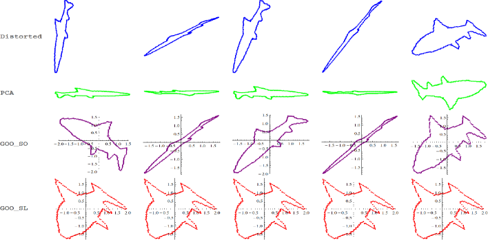
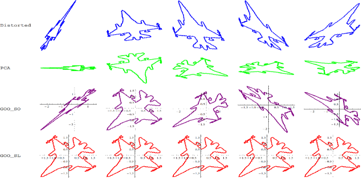
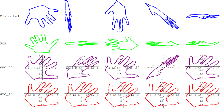
Fig. 3: This figures show the results of normalizing distorted point clouds by different methods. The rows marked with “Distorted” consist of distorted point clouds used as input to various normalization methods. The rows marked with “PCA” contain results of normalization by principal component analysis. It can be seen that the effects of rotational distortion have been partially eliminated, but results of shearing and squeezing remain. The rows marked with “GOO_SO” contain results of normalization using special orthogonal group in GOO. It can be seen that the effects of rotational distortion have been partially eliminated, but results of shearing and squeezing remain. The rows marked with “GOO_SL” contain results of normalization using Algorithm 60, where it can be seen that the algorithm can produce approximately the same point clouds after eliminating distortions like shearing, squeezing and rotation.

In Figure 4 we study the impact of number of points on the canonical form found by the GOO. We can see that though the number of points in the canonical form vary between 180 and 260, the canonical form is nearly the same, module different orientations. In this case although Step 2 in Algorithm 60 cannot completely eliminate the ambiguity of four possible orientations of point clouds, we can simply remove this ambiguity by enumerating all four possible orientations when doing comparison. This property means that when comparing shape of two point clouds, it is not necessary to require two point clouds to have exactly the same number of points when we are comparing based on the canonical forms.

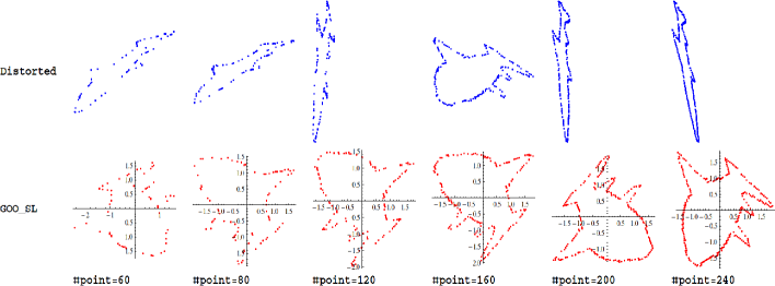
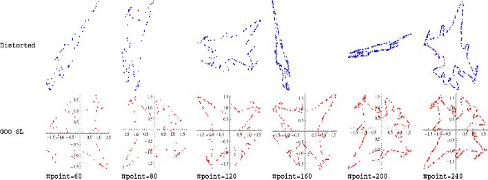
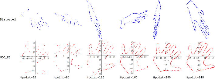
Fig. 4: The point clouds in rows marked with “Distorted” are the results of applying distortion generated by random special linear matrix to original point clouds. The point clouds in rows marked with “GOO_SL” are after normalization by special linear group. From left to right, the sparser point clouds are generated by sampling from the rightmost densest point cloud respectively. It can be seen that for all three examples, though density varies, the shape of the normalized point clouds remains stable, modulo four possible orientations.

8 Related work

In this section we discuss the related work not yet covered in the previous sections.

An early example of GOO is a so-called quadratic assignment problem [20] where the following optimization problem is studied:

$$\inf_{{\bf X}\in\Pi_{n}}\operatorname{tr}({\bf W}{\bf X}{\bf D}{\bf X}^{\top})\text{,}$$

where $\Pi_{n}$ is the permutation matrix group. Due to the combinatorial nature of $\Pi_{n}$, QAP is NP-hard. In contrast, we mainly work on non-combinatorial matrix groups in this paper.

In [27], a non-linear GOO is used to find texture invariant to rotation for 2D point cloud ${\bf M}\in{\mathbb{F}}^{n\times 2}$:

$$\inf_{{\bf G}\in\mathfrak{O}}\|\operatorname{Rasterize}(\operatorname{Poly}({\bf M}{\bf G}))\|_{*}\text{.}$$

As $\mathfrak{O}$ is a unit group, the optimization is well defined and the induced matrix decomposition is found to be useful as a rotation-invariant representation for texture. The same paper also considers finding homography-invariant representation for texture for 2D point cloud ${\bf M}\in{\mathbb{F}}^{n\times 2}$:

$$\inf_{{\bf G}\in\mathfrak{H},\;\mu(\operatorname{Poly}(\lambda{\bf M}{\bf G}))=\mathop{\operator@font const}\nolimits}\|\operatorname{Rasterize}[\operatorname{Poly}(\lambda{\bf M}{\bf G})]\|_{*}\text{.}$$

Note that here a coefficient $\lambda$ is intentionally added to ensure $\mu$ measure of the point cloud be preserved w.r.t. the action of ${\bf G}$.

In [10] the following formulation is used to get the Ky-Fan $k$-norm [9] of a matrix ${\bf M}\in{\mathbb{F}}^{m\times n}$ when $m\geq k$ and $n\geq k$:

$$\sup_{{\bf G}_{1}\in{\mathbb{F}}^{m\times k},{\bf G}_{1}^{\top}{\bf G}_{1}={\bf I}_{k},{\bf G}_{2}\in{\mathbb{F}}^{n\times k},{\bf G}_{2}^{\top}{\bf G}_{2}={\bf I}_{k}}\operatorname{tr}({\bf G}_{1}^{\top}{\bf M}{\bf G}_{2})\text{.}$$

Note that the above optimization is not a GOO when $k^{2}\neq mn$ as in that case ${\bf G}_{2}^{\top}\otimes{\bf G}_{1}^{\top}\in{\mathbb{F}}^{k^{2}\times mn}$ does not form a group.

9 Conclusion

In this paper, we have studied an optimization problem over the group orbit generated by action of group ${\mathfrak{G}}$ and referred to it as the Group Orbit Optimization (GOO). We have shown that SVD/QR/LU/Cholesky decomposition can be reformulated under the GOO framework as in Theorem 15. Moreover, we have used GOO to induce tensor decomposition in Theorem 43. The unified framework of GOO for matrix decomposition and tensor decomposition allows us to bridge them. In particular, we have presented Lemma 37, which relates the infimum of the tensor-based GOO with the infimum of GOO of the matrix unfolded to the tensor. Finally, we have applied GOO to point cloud data to demonstrate the use of data normalization in shape matching when objects are represented as point clouds.

Our work has demonstrated that the unified framework of GOO for data normalization is both of theoretical interests in providing a new perspective on matrix and tensor decompositions, and of practical interests in modeling and elimination of distortions present in real world data.

References

- [1] P-A Absil, Robert Mahony, and Rodolphe Sepulchre, Optimization algorithms on matrix manifolds, Princeton University Press, 2009.
- [2] Lieven De Lathauwer, Decompositions of a higher-order tensor in block terms—part ii: Definitions and uniqueness, SIAM J. Matrix Anal. Appl., 30 (2008), pp. 1033–1066.
- [3] J. Demmel, Applied Numerical Linear Algebra, SIAM, Philadelphia, 1997.
- [4] Ian L Dryden and Kanti V Mardia, Statistical shape analysis, vol. 4, John Wiley & Sons New York, 1998.
- [5] Alan Edelman, Tomás A Arias, and Steven T Smith, The geometry of algorithms with orthogonality constraints, SIAM journal on Matrix Analysis and Applications, 20 (1998), pp. 303–353.
- [6] G. H. Golub and C. F. Van Loan, Matrix Computations, The Johns Hopkins University Press, Baltimore, third ed., 1996.
- [7] Richard A Harshman, Foundations of the parafac procedure: models and conditions for an” explanatory” multimodal factor analysis, (1970).
- [8] Richard Hartley and Andrew Zisserman, Multiple view geometry in computer vision, Cambridge university press, 2003.
- [9] Roger A Horn and Charles R Johnson, Topics in matrix analysis, Cambridge university press, 1991.
- [10] Yao Hu, Debing Zhang, Jieping Ye, Xuelong Li, and Xiaofei He, Fast and accurate matrix completion via truncated nuclear norm regularization, Pattern Analysis and Machine Intelligence, IEEE Transactions on, 35 (2013), pp. 2117–2130.
- [11] Mariya Ishteva, Lieven De Lathauwer, P Absil, and Sabine Van Huffel, Dimensionality reduction for higher-order tensors: algorithms and applications, International Journal of Pure and Applied Mathematics, 42 (2008), p. 337.
- [12] Tamara G. Kolda, Orthogonal tensor decompositions, SIAM J. Matrix Anal. Appl., 23 (2001), pp. 243–255.
- [13] Tamara G. Kolda and Brett W. Bader, Tensor decompositions and applications, SIAM Rev., 51 (2009), pp. 455–500.
- [14] Akshay Krishnamurthy and Aarti Singh, Low-rank matrix and tensor completion via adaptive sampling, in Advances in Neural Information Processing Systems, 2013, pp. 836–844.
- [15] Lieven De Lathauwer, Bart De Moor, and Joos Vandewalle, A multilinear singular value decomposition, SIAM J. Matrix Anal. Appl., 21 (2000), pp. 1253–1278.
- [16] , On the best rank-1 and rank-(r1,r2,. . .,rn) approximation of higher-order tensors, SIAM J. Matrix Anal. Appl., 21 (2000), pp. 1324–1342.
- [17] , Computation of the canonical decomposition by means of a simultaneous generalized schur decomposition, SIAM J. Matrix Anal. Appl., 26 (2005), pp. 295–327.
- [18] Ji Liu, Przemyslaw Musialski, Peter Wonka, and Jieping Ye, Tensor completion for estimating missing values in visual data, IEEE Trans. Pattern Anal. Mach. Intell., 35 (2013), pp. 208–220.
- [19] John A Nelder and Roger Mead, A simplex method for function minimization, The computer journal, 7 (1965), pp. 308–313.
- [20] Sartaj Sahni and Teofilo Gonzalez, P-complete approximation problems, Journal of the ACM (JACM), 23 (1976), pp. 555–565.
- [21] Marco Signoretto, Lieven De Lathauwer, and Johan AK Suykens, Nuclear norms for tensors and their use for convex multilinear estimation, Submitted to Linear Algebra and Its Applications, 43 (2010).
- [22] Ryota Tomioka, Kohei Hayashi, and Hisashi Kashima, On the extension of trace norm to tensors, in NIPS Workshop on Tensors, Kernels, and Machine Learning, 2010, p. 7.
- [23] Lloyd N. Trefethen and David Bau III, Numerical Linear Algebra, SIAM, Philadelphia, 1997.
- [24] Ledyard R Tucker, Some mathematical notes on three-mode factor analysis, Psychometrika, 31 (1966), pp. 279–311.
- [25] Constantin Udriste, Convex functions and optimization methods on Riemannian manifolds, vol. 297, Springer, 1994.
- [26] Tong Zhang and Gene H. Golub, Rank-one approximation to high order tensors, SIAM J. Matrix Anal. Appl., 23 (2001), pp. 534–550.
- [27] Zhengdong Zhang, Arvind Ganesh, Xiao Liang, and Yi Ma, Tilt: transform invariant low-rank textures, International Journal of Computer Vision, 99 (2012), pp. 1–24.