Critical behavior and continuum scaling of $3D$ $Z(N)$ lattice gauge theories

Abstract:

Three-dimensional $Z(N)$ lattice gauge theories are studied numerically at finite temperature for $N$ = 5, 6, 8, 12, 13, 20 and for $N_{t}$=2,4,8. For each model the location of phase transitions and its critical indices are determined. The scaling of critical points with $N$ is proposed. The data obtained enable us to verify the scaling near the continuum limit for the $Z(N)$ models at finite temperatures.

1 Introduction

In this paper we focus on the phase structure of $Z(N)$ lattice gauge theories (LGTs), which are interesting on their own and can provide for useful insights into the universal properties of $SU(N)$ LGTs, being $Z(N)$ the center subgroup of $SU(N)$. The most general action for the $Z(N)$ LGT is

$$S_{\rm gauge}\ =\ \sum_{x}\sum_{n<m}\ \sum_{k=1}^{N}\beta_{k}\cos\left(\frac{2\pi k}{N}\left(s_{n}(x)+s_{m}(x+e_{n})-s_{n}(x+e_{m})-s_{m}(x)\right)\right)\ .$$ (1)

Gauge fields take on values $s_{n}(x)=0,1,\cdots,N-1$ and are defined on the links of the lattice. $Z(N)$ gauge models can generally be divided into two classes: standard Potts models (all $\beta_{k}$ equal) and vector models (otherwise). The conventional vector model corresponds to $\beta_{k}=0$ for all $k>1$. For $N=2,\ 3$ the Potts and vector models are equivalent.

An extended description of the phase structure of $Z(N)$ LGTs in three dimension can be found in [1, 2, 3]. In those papers we explored the phase structure of the vector $Z(N)$ LGTs for $N>4$. We considered first an anisotropic lattice in the limit where the spatial coupling vanishes [1] and were able to present both renormalization group (RG) and numerical evidences for the existence of two BKT-like phase transitions: a (i) first transition, from a symmetric, confining phase to an intermediate phase, where the $Z(N)$ symmetry is enhanced to $U(1)$ symmetry; (ii) a second transition, from the intermediate phase to a phase with broken $Z(N)$ symmetry. We computed also some critical indices, which appear to agree with the corresponding indices of $2D$ $Z(N)$ spin models, thus giving further support to the Svetitsky-Yaffe conjecture [4]. In particular, we found that the magnetic critical index $\eta$ at the first transition, $\eta^{(1)}$, takes the value 1/4 as in $2D$ $XY$, while its value at the second transition, $\eta^{(2)}$, is equal to $4/N^{2}$. Then, we extended our analysis to the full isotropic $3D$ $Z(N)$ LGT at finite temperature [2] and confirmed by numerical Monte Carlo simulations [2] that the full gauge models with $N>4$ possess two phase transitions of the BKT type, with critical indices coinciding with those of $2D$ vector spin models.

Here we extend the study of Ref. [2] to other values of $N$ and to $N_{t}=8$ and aim at checking the scaling near the continuum limit and at establishing the scaling formula for critical points with $N$. In particular, the theory of dimensional cross-over [5] explains how critical couplings and indices of a finite temperature LGT (finite $N_{t}$) approach critical couplings and indices of the corresponding zero-temperature theory ($N_{t}\to\infty$). This provides us with a way to crosscheck our zero-temperature results [3] and thus predict the critical temperature in the continuum limit.

The standard approach for studying a BKT transition consists in using Binder cumulants and susceptibilities of the Polyakov loop to determine critical couplings and critical indices. Here, as in Ref. [2], we follow a different strategy: we move to a dual formulation and use Binder cumulants and susceptibilities of dual $Z(N)$ spins. This implies that (i) the critical behavior of dual spins is reversed with respect to that of Polyakov loops, namely the spontaneously-broken ordered phase is mapped to the symmetric phase and vice versa; (ii) the magnetic critical indices $\eta$ are interchanged, whereas the index $\nu$ is expected to be the same (=1/2) at both transitions (see Ref. [2] for details). The obvious advantage of this approach is that cluster algorithms become available, with considerable speed up in the numerical procedure.

2 Theoretical setup

The $3D$ $Z(N)$ gauge theory on an anisotropic $3D$ lattice $\Lambda$ can generally be defined as

$$Z(\Lambda;\beta_{t},\beta_{s};N)\ =\ \prod_{l\in\Lambda}\left(\frac{1}{N}\sum_{s(l)=0}^{N-1}\right)\ \prod_{p_{s}}Q(s(p_{s}))\ \prod_{p_{t}}Q(s(p_{t}))\;,$$ (2)

where the link angles $s(l)$ are combined into the conventional plaquette angle

$$s(p)\ =\ s_{n}(x)+s_{m}(x+e_{n})-s_{n}(x+e_{m})-s_{m}(x)\ .$$ (3)

Here, $e_{n}$ ($n=0,1,2$) denotes a unit vector in the $n$-th direction and the notation $p_{t}$ ($p_{s}$) stands for the temporal (spatial) plaquettes. Periodic boundary conditions (BC) on gauge fields are imposed in all directions. The most general $Z(N)$-invariant Boltzmann weight with $N-1$ different couplings is

$$Q(s)\ =\ \exp\left[\sum_{k=1}^{N-1}\beta_{p}(k)\cos\frac{2\pi k}{N}s\right]\ .$$ (4)

The Wilson action corresponds to the choice $\beta_{p}(1)=\beta_{p}$, $\beta_{p}(k)=0,k=2,...,N-1$, which is the one adopted in this work. Furthermore, we will consider an isotropic lattice: $\beta_{s}=\beta_{t}=\beta$.

Our study is based on the mapping of the gauge model to a generalized $3D$ $Z(N)$ spin model on a dual lattice $\Lambda_{d}$, whose action is

$$S\ =\ \sum_{x}\ \sum_{n=1}^{3}\sum_{k=1}^{N-1}\ \beta_{k}\ \cos\left(\frac{2\pi k}{N}\left(s(x)-s(x+e_{n})\right)\right)\ .$$ (5)

The dual mapping is realized once one specifies the relationship between the original gauge coupling $\beta$ and the dual effective couplings $\beta_{k}$. This has been done in Ref. [2] (see also Ref. [6]) and the result is

$$\beta_{k}\ =\ \frac{1}{N}\sum_{p=0}^{N-1}\ln\left[\frac{Q_{d}(p)}{Q_{d}(0)}\right]\ \cos\left(\frac{2\pi pk}{N}\right)\ .$$ (6)

For $N=5$ it can be seen explicitly [2] that $|\beta_{1}|\gg|\beta_{2}|$, thus suggesting that the $3D$ vector spin model with only $\beta_{1}$ non-vanishing gives already a reasonable approximation of the gauge model. Moreover the weak and the strong coupling regimes are interchanged, i.e. when $\beta\to\infty$ the effective couplings $\beta_{k}\to 0$ and, therefore, the ordered symmetry-broken phase is mapped to a symmetric phase with vanishing magnetization of dual spins, whereas the symmetric phase at small $\beta$ becomes an ordered phase where the dual magnetization is non-zero. The interchange of phases under the dual mapping is not a special feature of $N=5$, but is rather a general property valid for any $N$. In Ref. [2] it was also discussed that at the critical point $\beta_{\rm c}^{(1)}$ of the first transition of the LGT (from the symmetric to the intermediate phase), the dual correlation function scales with a critical index $\eta$ equal to the index $\eta^{(2)}=4/N^{2}$ of the Polyakov loop correlator in the LGT, while at the critical point $\beta_{\rm c}^{(2)}$ of the second transition in the LGT (from the intermediate to the broken phase), it scales with a critical index $\eta$ equal to the index $\eta^{(1)}=1/4$ of the Polyakov loop correlator in the LGT. This can be proved in the Villain formulation of the $2D$ theory and only conjectured (but confirmed numerically) in the $3D$ case [2].

3 Numerical setup and results

The $3D$ $Z(N)$ spin model, dual of the $3D$ $Z(N)$ Wilson LGT, has been simulated by means of a cluster algorithm on $N_{t}\times L\times L$ lattices with periodic BC. The system has been studied for $N$ = 5, 6, 8, 12, 13 and 20 on lattices with the temporal extension $N_{t}$=2, 4, 8. With respect to our previous work [2], we considered new values of $N$ (6, 8, 12, 20) and included also $N_{t}=8$. We focused on the following observables:

• complex magnetization $M_{L}=|M_{L}|e^{i\psi}$, with $M_{L}\ =\ \sum_{x\in\Lambda}\exp\left(\frac{2\pi i}{N}s(x)\right)$, where we stress that $s(x)$ is a dual spin variable;

• real part of the rotated magnetization, $M_{R}=|M_{L}|\cos(N\psi)$, and normalized rotated magnetization, $m_{\psi}=\cos(N\psi)$;

• susceptibilities of $M_{L}$ and $M_{R}$, $\chi_{L}^{(M)}$, $\chi_{L}^{(M_{R})}$:   $\chi_{L}^{(\mathbf{\cdot})}\ =\ L^{2}N_{t}\left(\left<\mathbf{\cdot}^{2}\right>-\left<\mathbf{\cdot}\right>^{2}\right)$;

• Binder cumulants $U_{L}^{(M)}$ and $B_{4}^{(M_{R})}$:   $U_{L}^{(M)}\ =\ 1-\frac{\left\langle\left|M_{L}\right|^{4}\right\rangle}{3\left\langle\left|M_{L}\right|^{2}\right\rangle^{2}}\;,\;\;\;\;\;B_{4}^{(M_{R})}\ =\ \frac{\left\langle\left|M_{R}-\left\langle M_{R}\right\rangle\right|^{4}\right\rangle}{\left\langle\left|M_{R}-\left\langle M_{R}\right\rangle\right|^{2}\right\rangle^{2}}$.

To determine the critical couplings of the second transition point, $\beta_{\rm c}^{(2)}$, we have looked for the value of $\beta$ at which the curves giving the Binder cumulant $U_{L}^{(M)}(\beta)$ on lattices with different size $L$ “intersect” (see Ref. [7] for details). The same method can in principle be used for the couplings of the first transition, $\beta_{\rm c}^{(1)}$, using either the Binder cumulant $B_{4}^{(M_{R})}$ or $m_{\psi}$; it turned out, however, that the precision required by this method on these observables could not be met with a sensible simulation time. For this reason, as the position of the first critical point we used our previous determinations given in Ref. [2], where $\beta_{\rm c}^{(1)}$ was taken as the value of $\beta$ at which $B_{4}^{(M_{R})}$ and $m_{\psi}$ plotted versus $(\beta-\beta_{\rm c}^{(1)}){\ln L}^{1/\nu}$ show the best overlap for different values of $L$. The results of the determinations of $\beta_{\rm c}^{(1)}$ and $\beta_{\rm c}^{(2)}$ are summarized in Table 1.

Table 1: Values of $\beta_{\rm c}^{(1)}$ and $\beta_{\rm c}^{(2)}$ obtained for various $N_{t}$ in $3D$ $Z(N)$ with $N=5,\ 6,\ 8,\ 12,\ 13$ and 20.

$N$	$N_{t}$	$\beta_{\rm c}^{(1)}$	$\beta_{\rm c}^{(2)}$
5	2	1.617(2)	1.6972(14)
5	4	1.943(2)	1.9885(15)
5	6	2.05(1)	2.08(1)
5	8	2.085(2)	2.1207(9)
5	12	2.14(1)	2.16(1)
6	2	-	2.3410(15)
6	4	-	2.725(12)
6	8	-	2.899(4)
8	2	-	3.8640(10)
8	4	2.544(8)	4.6864(15)
8	8	3.422(9)	4.9808(5)

$N$	$N_{t}$	$\beta_{\rm c}^{(1)}$	$\beta_{\rm c}^{(2)}$
12	2	-	8.3745(5)
12	4	-	10.240(7)
12	8	-	10.898(5)
13	2	1.795(4)	9.735(4)
13	4	2.74(5)	11.959(6)
13	8	3.358(7)	12.730(2)
20	2	-	22.87(4)
20	4	2.57(1)	28.089(3)
20	8	3.42(5)	29.758(6)

For the critical couplings at the second transition, $\beta_{\rm c}^{(2)}$, where determinations for many values of $N$ are available, we tried to find a simple scaling dependence with $N$ at fixed $N_{t}$. From the solution of the renormalization group equations for $2D$ $Z(N)$ spin model, we know that in that model $\beta_{\rm c}^{(2)}(N)$ grows as $N^{2}$ for large $N$ [8]. In [1] we have found that this is the case also for the $3D$ $Z(N)$ LGT at finite temperature, at least in the strong coupling limit. Taking inspiration from Ref. [9], we started from a scaling law written in the form $\beta_{\rm c}^{(2)}(N)=A/(1-\cos{2\pi/N})$. Then, considering that the next non-negligible correction comes at the order $1/N^{2}$, we added a second term and ended up with the same scaling function we used in the zero-temperature case [3],

$$\beta_{\rm c}^{(2)}(N)=\frac{A}{(1-\cos{2\pi/N})}+B(1-\cos{2\pi/N})\;.$$

In Table 2 we report the values of the parameters $A$ and $B$ for $N_{t}=2,\ 4,\ 8$, while Figs. 1 shows the fitting functions against numerical data.

Table 2: Parameters of the scaling with $N$ of the second transition point, $\beta_{\rm c}^{(2)}=A/{(1-\cos{2\pi/N})}+B(1-\cos{2\pi/N})$ at fixed $N_{t}$.

$N_{t}$	$A$	$B$	$\chi^{2}_{\rm r}$
2	1.1194(11)	0.141(24)	209
4	1.37440(60)	-0.0046(88)	18.2
8	1.45745(57)	0.0155(53)	16.1

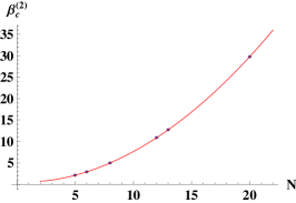
Figure 1: Scaling function $A/(1-\cos{2\pi/N})+B(1-\cos{2\pi/N})$ versus data for $\beta_{\rm c}^{(2)}$ at $N_{t}=2,\ 4,\ 8$ (from left to right).

Finding the continuum limit of the finite temperature theory in the first or in the second transition amounts to extrapolate the corresponding critical couplings, $\beta_{\rm c}^{(1)}$ or $\beta_{\rm c}^{(2)}$, to the limit $N_{t}\to\infty$ at fixed $N$. The theory of dimensional cross-over [5] suggests the fitting function to be used:

$$\beta_{\rm c}^{(1,2)}(N_{t})=\beta_{{\rm c},\ T=0}^{(1,2)}-(N_{t}aT_{\rm c})^{-1/\nu}\;,$$ (7)

where $\beta_{{\rm c},\ T=0}^{(1,2)}$ and $\nu$ are the critical couplings and the critical index of the zero-temperature theory. Since we know that, for any $N$, the $3D$ $Z(N)$ LGT at zero-temperature exhibits only one phase transition, with the critical index $\nu$ depending on the side from which the transition is approached [3], we expect that, for a given $N$, the fit parameters $\beta_{{\rm c},\ T=0}^{(1)}$ and $\beta_{{\rm c},\ T=0}^{(2)}$ take the same value and agree with the zero-temperature critical coupling at the same $N$. As for the fit parameter $\nu$, we expect it to agree with the value of the critical index $\nu$ at one of the two sides of the zero-temperature transition. We fitted with the function given in (7) our data for the critical couplings $\beta_{\rm c}^{(1)}(N_{t})$ at $N$=5 and for the critical couplings $\beta_{\rm c}^{(2)}(N_{t})$ at $N$=5, 6, 8, 12, 13, 20 (see Table 3). In some cases in the fit we fixed either $\beta_{{\rm c},\ T=0}^{(1,2)}$ or $\nu$, or both, at the values known from the zero-temperature theory [3]. The scenario which emerges from the inspection of Tables 3 is that, despite the large reduced chi-squared obtained in a few cases, the agreement between the fit parameters $\beta_{{\rm c},\ T=0}^{(1,2)}$ and the known zero-temperature critical couplings [3] is satisfactory. As for the value of the fit parameter $\nu$, results are not precise enough to discriminate between the known values of the critical index $\nu$ of the zero-temperature theory at one or the other side of the transition [3]. This analysis allows us for the determination of the critical temperature $aT_{\rm c}$ in the continuum limit for all the values of $N$ considered in this work.

Table 3: Results of the fit of $\beta_{\rm c}^{(1)}(N_{t})$ for $N=$ and of $\beta_{\rm c}^{(2)}(N_{t})$ for $N$=5, 6, 8, 12, 13, 20 with the function (7). Parameters are given without errors when their values were fixed at the known results of the $T=0$ corresponding theory [3] (for the $\nu$ index we considered both the values at the left and at the right of the $T=0$ critical point). Parameters are given with a (-) mark when their errors are unavailable and with a ^∗ mark when obtained from fits on data with $N_{t}=4,\ 8$ only (in general, $N_{t}=2,\ 4,\ 8$ were considered).

$N$	$aT_{\rm c}$	$\beta_{{\rm c},\ T=0}^{(1)}$	$\nu$	$\chi_{\rm r}^{2}$
	0.790(5)	2.198(9)	0.84(3)	1.21
	0.764(14)	2.144(9)	0.670	23.1
	0.758(16)	2.135(11)	0.640	33.6
5	0.786(7)	2.17961	0.788(10)	2.66
	0.722(16)	2.17961	0.670	105
	0.709(19)	2.17961	0.640	171

$N$	$aT_{\rm c}$	$\beta_{{\rm c},\ T=0}^{(2)}$	$\nu$	$\chi_{\rm r}^{2}$
	0.868(-)	2.23055(-)	0.877(-)	-
	0.813(27)	2.177(12)	0.670	158
	0.803(30)	2.170(14)	0.640	223
5	0.825(38)	2.17961	0.692(45)	131
	0.810(13)	2.17961	0.670	81.8
	0.776(31)∗	2.17961	0.670	74.2∗
	0.789(17)	2.17961	0.640	161
	0.731(18)∗	2.17961	0.640	31.4∗
	0.6814(-)	3.04317(-)	0.876(-)	-
	0.6769(76)	2.977(10)	0.674	5.02
	0.6740(85)	2.969(12)	0.642	6.90
6	0.6832(46)	3.00683	0.768(15)	1.14
	0.6573(47)	3.00683	0.674	22.6
	0.572(13)∗	3.00683	0.674	1.44∗
	0.6487(60)	3.00683	0.642	40.6
	0.542(21)∗	3.00683	0.642	4.48∗
	0.42330(-)	5.14422(-)	0.674(-)	-
	0.42378(12)	5.14299(25)	0.672	0.19
	0.4316(22)	5.1225(46)	0.637	66.5
8	0.4294(12)	5.12829	0.648(6)	33.0
	0.4287(39)	5.12829	0.672	321
	0.4427(39)∗	5.12829	0.672	177∗
	0.4298(19)	5.12829	0.637	86.1
	0.4216(10)∗	5.12829	0.637	2.21∗

$N$	$aT_{\rm c}$	$\beta_{{\rm c},\ T=0}^{(2)}$	$\nu$	$\chi_{\rm r}^{2}$
	0.24728(-)	11.2566(-)	0.674(-)	-
	0.24559(13)	11.2640(23)	0.670	0.22
	0.25615(72)	11.218(12)	0.640	6.18
12	0.2602(32)	11.1962	0.630(11)	14.2
	0.24954(28)	11.1962	0.670	89.8
	0.2619(87)∗	11.1962	0.670	55.5∗
	0.25742(10)	11.1962	0.640	12.7
	0.2597(51)∗	11.1962	0.640	21.3∗
	0.22433(-)	13.1391(-)	0.654(-)	-
	0.21872(53)	13.1656(56)	0.671	5.88
	0.22851(40)	13.1199(42)	0.642	3.40
13	0.2310(12)	13.1077	0.635(4)	8.86
	0.2225(30)	13.1077	0.671	314
	0.2342(62)∗	13.1077	0.671	113∗
	0.22928(67)	13.1077	0.642	16.0
	0.2311(24)∗	13.1077	0.642	19.2∗
	0.144857(-)	30.5427(-)	0.608(-)	-
	0.1297(37)	30.73(10)	0.673	147
	0.1356(24)	30.658(64)	0.647	58.8
20	0.1357(26)	30.6729	0.642(19)	58.2
	0.13171(98)	30.6729	0.673	97.3
	0.13199(13)∗	30.6729	0.673	1.57∗
	0.13506(54)	30.6729	0.647	31.0
	0.13519(49)∗	30.6729	0.647	23.9∗

Some critical indices at the two transitions in the $3D$ $Z(N)$ LGT at finite temperature can be extracted by the standard FSS analysis. In particular, the behavior on the lattice size $L$ of the standard magnetization $M_{L}$ and of its susceptibility at the second transition allows to extract the indices $\beta/\nu$ and $\gamma/\nu$ through a fit with the functions

$$M_{L}=A_{M_{L}}L^{-\beta/\nu}\;,\;\;\;\;\;\chi_{M_{L}}=A_{\chi_{M_{L}}}L^{\gamma/\nu}\;.$$ (8)

Similarly, the behavior on $L$ of the rotated magnetization $M_{R}$ and of its susceptibility at the first transition point allow the extraction of the same critical indices at that transition. Thereafter, the hyperscaling relation $2\beta/\nu+\gamma/\nu=2$ can be checked and the magnetic index $\eta=2-\gamma/\nu$ can be extracted at both transitions. Our results are reported in Ref. [7] and show that the hyperscaling relation is generally satisfied and the critical index $\eta$ generally takes values compatible with 1/4 at the second transition and with $4/N^{2}$ at the first transition, in agreement with the expectations.

4 Summary

This paper completes our study of the critical behavior of $3D$ $Z(N>4)$ lattice gauge theories both at finite temperatures. We have found that in all $Z(N)$ vector models two BKT-like phase transitions occur at finite temperatures if $N>4$. In all cases studied, the results for the critical indices suggest that finite-temperature $Z(N)$ lattice models belong to the universality class of two-dimensional $Z(N)$ vector spin models, in agreement with the Svetitsky-Yaffe conjecture. Furthermore, the available results for many values of $N$ allowed us to propose and check some scaling formulas for the critical point of the second phase transition. Combining the results of the present paper with those for the index $\nu$ obtained by us at zero temperature in Ref. [3] enabled us to check the continuum scaling and to predict the approximate value for $aT_{c}$ in the continuum limit.

References

- [1] O. Borisenko, V. Chelnokov, G. Cortese, R. Fiore, M. Gravina, A. Papa, I. Surzhikov, Phys. Rev. E 86 (2012) 051131; PoS LATTICE 2012 270 [arXiv:1212.1051 [hep-lat]].
- [2] O. Borisenko, V. Chelnokov, G. Cortese, M. Gravina, A. Papa, I. Surzhikov, Nucl. Phys. B 870 (2013) 159; PoS LATTICE 2013 463 [arXiv:1310.1039 [hep-lat]].
- [3] O. Borisenko, V. Chelnokov, G. Cortese, M. Gravina, A. Papa, I. Surzhikov, Nucl. Phys. B 879 (2014) 80; PoS LATTICE 2013 347 [arXiv:1311.0471 [hep-lat]].
- [4] B. Svetitsky, L. Yaffe, Nucl. Phys. B 210 (1982) 423.
- [5] M. Caselle, M. Hasenbusch, M. Panero, JHEP 0301 (2003) 057; M. Caselle, M. Hasenbusch, Nucl. Phys. B 470 (1996) 435.
- [6] A. Ukawa, P. Windey, A.H. Guth, Phys. Rev. D 21 (1980) 1013.
- [7] O. Borisenko, V. Chelnokov, M. Gravina, A. Papa, Nucl. Phys. B 888 (2014) 52.
- [8] O. Borisenko, V. Chelnokov, G. Cortese, R. Fiore, M. Gravina, A. Papa, Phys. Rev. E 85 (2012) 021114.
- [9] G. Bhanot and M. Creutz, Phys. Rev. D 21 (1980) 2892.