Resolving the Clumpy Structure of the Outflow Winds in the Gravitationally Lensed Quasar SDSS J1029+2623

Abstract

We study the geometry and the internal structure of the outflowing wind from the accretion disk of a quasar by observing multiple sightlines with the aid of strong gravitational lensing. Using Subaru/HDS, we performed high-resolution ($R$ $\sim$ 36,000) spectroscopic observations of images A and B of the gravitationally lensed quasar SDSS J1029+2623 (at $z_{em}$ $\sim$ 2.197) whose image separation angle, $\theta$ $\sim$ 22${}^{\prime\prime}\!\!$.5, is the largest among those discovered so far. We confirm that the difference in absorption profiles in the images A and B discovered by Misawa et al. (2013) remains unchanged since 2010, implying the difference is not due to time variability of the absorption profiles over the delay between the images, $\Delta t$ $\sim$ 744 days, but rather due to differences along the sightlines. We also discovered time variation of C IV absorption strength in both images A and B, due to change of ionization condition. If a typical absorber’s size is smaller than its distance from the flux source by more than five orders of magnitude, it should be possible to detect sightline variations among images of other smaller separation, galaxy-scale gravitationally lensed quasars.

1 INTRODUCTION

Outflowing winds from accretion disks, accelerated by radiation force (Murray et al., 1995; Proga, Stone, & Kallman, 2000), magnetocentrifugal force (Everett, 2005; de Kool & Begelman, 1995), and/or thermal pressure (Balsara & Krolik, 1993; Krolik & Kriss, 2001; Chelouche & Netzer, 2005), are a key evolutionary link between quasars and their host galaxies. The disk outflow plays an important role as 1) it extracts angular momentum from the accretion disk, leading to growth of black holes (Blandford & Payne, 1982; Konigl & Kartje, 1994; Everett, 2005), 2) it provides energy and momentum feedback and inhibits star formation activity (e.g., Springel, Di Matteo, & Hernquist, 2005), and 3) it induces metal enrichment of intergalactic medium (IGM) (Hamann et al., 1997a; Gabel et al., 2006). Outflowing matter has been detected through blueshifted absorption lines in $\sim$70% of quasar spectra (Hamann et al., 2012). These are usually classified as intrinsic absorption lines, and distinguished from intervening absorption lines that originate in foreground galaxies or in the IGM. Thus, intrinsic absorption lines are powerful and unique tool to probe the outflows in quasars. However, the main challenge in their study is that these are traceable along only single sight-lines (i.e., a one dimensional view alone) toward the nucleus for each quasar, whereas the absorber’s physical conditions likely depend strongly on polar angle (e.g., Ganguly et al., 2001; Elvis, 2000).

Multiple images of quasars produced by the gravitational lensing effect provide a unique pathway for studying the multiple sightlines, a technique frequently applied for intervening absorbers (e.g., Crotts & Fang 1998; Rauch et al. 1999; Lopez et al. 2005). It is clear that lensed quasars with larger image separation angles have more chance of detecting structural differences in the outflow winds in the vicinity of the quasars themselves. In this sense, the following three lensed quasars are the most promising site for our study as they are lensed by a cluster of galaxies rather than a single massive galaxy: SDSS J1004+4112 with separation angle of $\theta$ $\sim$ 14${}^{\prime\prime}\!\!$.6 (Inada et al., 2003), SDSS J1029+2623 with $\theta$ $\sim$ 22${}^{\prime\prime}\!\!$.5 (Inada et al., 2006; Oguri et al., 2008), and SDSS J2222+2745 with $\theta$ $\sim$ 15${}^{\prime\prime}\!\!$.1 (Dahle et al., 2013). Green (2006) proposed that the differences in emission line profiles between the lensed images of SDSS J1004+4112 can be explained by differential absorptions along each sight-line although no absorption features are detected.

There are clear absorption features detected at the blue wings of the C IV, N V, and Ly$\alpha$ emission lines of other lensed quasar, SDSS J1029+2623 at $z_{em}$ $\sim$ 2.197, the current record-holding large-separation quasar lens, in low/medium resolution spectra (Inada et al., 2006; Oguri et al., 2008). Misawa et al. (2013) obtained high-resolution spectra of the brightest two images (i.e., images A and B), and carefully deblended the C IV and N V absorption lines into multiple narrower components. They show several clear signs supporting an origin in the outflowing wind rather than in foreground galaxies or the IGM (Misawa et al., 2013): i) partial coverage, i.e., the absorbers do not cover the background flux source completely along our sightline, ii) line-locking, iii) large velocity distribution (FWHM $\geq$1000 km/s), and iv) a small ejection velocity from the quasar. Misawa et al. (2013) also discovered a clear difference in parts of these lines between the images A and B in all C IV, N V, Ly$\alpha$ absorption lines, which can be explained by the following two scenarios: (a) intrinsic time variability of the absorption features over the time delay of the two images (e.g., Chartas et al., 2007), and (b) a difference in the absorption levels between the different sight-lines of the outflowing wind (e.g., Chelouche, 2003; Green, 2006). With a single epoch observation, we cannot distinguish these scenarios.

In this letter, we present results from new spectroscopic observations of SDSS J1029+2623 conducted $\sim$4 years later with the goal of conclusively determining the origin of the difference in the absorption features. We also examine the global and internal structure of the outflow. Observations and data reduction are described in §2, and results and discussion are in §3 and §4.

2 OBSERVATIONS and DATA REDUCTION

We observed the images A and B of SDSS J1029+2623 with Subaru/HDS on 2014 April 4 (the 2014 data, hereafter), 1514 days after the previous observation on February 2010 (the 2010 data; Misawa et al. 2013). The time interval between the observations is longer than the time delay between images A and B, $\Delta t$ $\sim$ 744 days in the sense of A leading B (Fohlmeister et al., 2013). We have taken high-resolution spectra ($R$ $\sim$ 36,000) with a slit width of $1.\!\!^{\prime\prime}0$, while Misawa et al. (2013) took $R$ $\sim$ 30,000 spectra using $1.\!\!^{\prime\prime}2$ slit width. The wavelength coverage is 3400–4230 Å on the blue CCD and 4280–5100 Å on the red CCD, which covers Ly$\alpha$, N V, Si IV, and C IV absorption lines at $z_{abs}$ $\sim$ $z_{em}$. We also sampled every 4 pixels in both spatial and dispersion directions (i.e., $\sim$0.05Å per pixel) to increase S/N ratio. The total integration time is 11400 s and the final S/N ratio is about 14 pix^-1 for both of the images.

We reduced the data in a standard manner with the software IRAF. Wavelength calibration was performed using a Th-Ar lamp. We applied flux calibrations for quasar spectra using the spectrophotometric standard star Feige34. We did not adjust a spectral resolution of the 2014 spectra ($R$ $\sim$ 36,000) to the 2010 ones ($R$ $\sim$ 30,000) before comparing them, because a typical line width of each absorption component after deblending into multiple narrower components is large enough (FWHM $\geq$ 10 km s^-1; Misawa et al. 2013) to ignore the influence of spectral resolution.

3 RESULTS

Here, we examine the time variability of Ly$\alpha$, N V, and C IV lines. Although Si IV is also detected, we cannot use it for the analysis because the Si IV line is severely contaminated by intervening Si II and C IV lines at lower redshift. For the purpose of comparing absorption profiles, we increase the S/N ratio by resampling the spectra every 0.5Å. For a more quantitative test, we also compare the flux difference between the two spectra to 3$\sigma$ flux uncertainty.

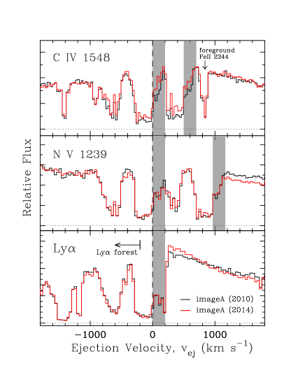
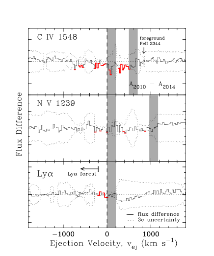
Figure 1: Comparison of the C IV, N V, and Ly$\alpha$ absorption profiles taken in 2010 (black) and 2014 (red) toward the image A of SDSS J1029+2623. (Left) The horizontal axis denotes ejection velocity relative to the quasar emission redshift ($z_{em}$ $\sim$ 2.197). The vertical axis flux scale is arbitrary. The shaded regions cover the $C_{1}$ of Ly$\alpha$ line and the doublets of C IV and N V lines while the other regions are the $C_{2}$. Intervening absorption lines that are not related to the outflow are marked with arrows and transition names. (Right) Comparison of flux difference between two spectra (solid histogram) with flux uncertainty (dotted histogram). Spectral regions where absorption line show variation in more than 3$\sigma$ level are marked with red histogram, except for Ly$\alpha$ forest and intervening absorption lines.

As shown in Figure 1, we did not find any time variations either in Ly$\alpha$ or N V absorption lines. But C IV lines in both of the images A and B showed clear variation in its line strength by more than the 3$\sigma$ level, without any change in line profiles.

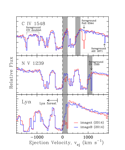
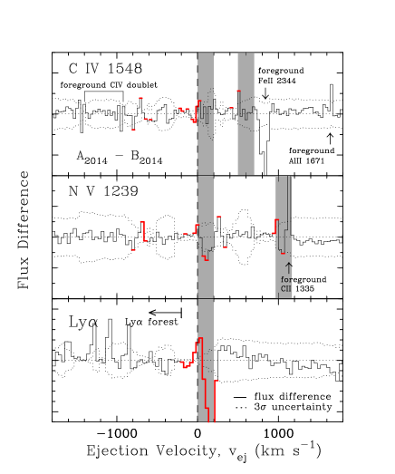
Figure 2: Same as Figure 1 but for the images A (red) and B (blue) of the 2014 spectra. The C IV doublet at $v_{ej}$ $\sim$ $-$1400 km s^-1, which shows $\geq$ 3$\sigma$ difference, is probably an intervening absorption line because the profile is narrow and the flux at the line center approaches close to zero before sampling. The profile difference in the shaded regions between the images A and B detected in the 2010 data (Misawa et al., 2013) still remains in the 2014 data.

In the 2010 spectra, Misawa et al. (2013) discovered a clear difference in parts of C IV, N V, and Ly$\alpha$ absorption lines at an ejection velocity of $v_{ej}$ $\sim$ 0 – 200 km s^-1 between the images A and B. The difference still remains at $\geq$ 3$\sigma$ level in the 2014 spectra, except for the C IV absorption lines for which the difference between images A and B is no longer significant (Figure 2). Thus, absorption components at $v_{ej}$ $\sim$ 0 – 200 km s^-1 (shaded regions in Figures 1 and 2) probably have a different origin from the other absorption components, as suggested in Misawa et al. (2013). We call the former and the latter components as Components 1 and 2 ($C_{1}$ and $C_{2}$, hereafter), respectively, and distinguish them in the discussion below.

4 DISCUSSION

In this section, we discuss the difference between the images A and B, the origin of the time variation seen in the C IV lines between the 2010 and the 2014 data, and then the detectability of the sightline variation for quasar images with smaller separations, lensed by a single galaxy.

4.1 Difference between the Images A and B

Misawa et al. (2013) presented two plausible scenarios that explain the sightline variation of the $C_{1}$: (a) time variability over the time delay between the images, $\Delta t$ $\sim$ 744 days, and (b) the difference in the absorption levels between two sightlines. With our new data, we can reject the first scenario because $C_{1}$ is again detected only in the image A as in the 2010 data. If this is due to time variation, the $C_{1}$ has to decrease (from the image A to B in 2010), increase (from the image B in 2010 to the image A in 2014), and then decrease again (from the image A to B in 2014), which requires an unlikely fine-tuning. Although sightline variations are often observed in intervening absorption lines (e.g., Crotts & Fang, 1998; Rauch et al., 1999; Lopez et al., 2005), the $C_{1}$ in the image A should have its origin in intrinsic absorber because it shows partial coverage (Misawa et al., 2013) and time variation (this study). Thus, the geometry of the outflow is such that the $C_{1}$ covers only sightline to the image A, while the $C_{2}$ covers both sightlines of the images A and B.

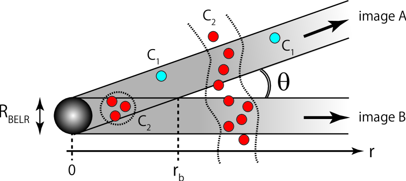
Figure 3: Possible locations of the $C_{1}$ and $C_{2}$ absorbers toward our sightlines. The large sphere represents the broad emission line region as a background flux source, while small blue and red filled circles are the $C_{1}$ and $C_{2}$ absorbers. The $C_{1}$ absorber always locates on only the sightline toward the image A, regardless of its distance. $C_{2}$ locates on both sightlines toward the images A and B or has a filamentary (or sheet-like) structure consisting of number of small clumpy clouds. The boundary distance ($r_{b}$) is the distance at which the two sightlines become fully separated with no overlap.

A possible structure of the outflow is shown in Figure 3. The $C_{1}$ absorber covers only the sightline toward image A but not image B, regardless of its distance ($r$) from the flux source. The size of the absorbing cloud ($d_{cloud}$) should be smaller than the size of the flux source (because of partial coverage) and also smaller than the physical distance between the sightlines of the lensed images, i.e., $d_{cloud}$ $\leq$ $r\theta$ to avoid covering both sightlines. Here, we assume the separation angle of the two sightlines from the flux source is very similar to that seen from us. On the other hand, $C_{2}$ has two possible origins: a) small gas clouds close to the flux source and b) filamentary (or sheet-like) structure made of multiple clumpy gas clouds (Misawa et al., 2013). In either case, both sightlines A and B need to be covered. We will discuss these further in Section 4.3.

4.2 Origin of Time Variation in C IV Lines

Time variability is frequently detected in broad absorption lines (BALs) with line widths of $\geq$ 2,000 km s^-1 (e.g., Gibson et al. 2008; Capellupo et al. 2013; Trevese et al. 2013). Some narrower intrinsic absorption lines (NALs and mini-BALs) are also known to be variable (e.g., Wise et al. 2004; Narayanan et al. 2004; Misawa et al. 2014). There are several explanations for the time variation, including gas motion across our line of sight (e.g., Hamann et al., 2008; Gibson et al., 2008), changes of the ionization condition (e.g., Hamann et al., 2011; Misawa et al., 2007b), and a variable scattering material that redirect photons around the gas clouds (e.g., Lamy & Hutsemékers, 2004). These mechanisms are not applicable to intervening absorbers because they have larger sizes (i.e., gas motion and photon redirection do not work) and lower densities (i.e., the variability time scale due to ion recombination is too long to observe over several years), compared to intrinsic absorbers as noted in Narayanan et al. (2004).

In our monitoring campaign, only C IV absorption lines show clear time variation in both of the images. The absorption strength is seen to weaken over the entire wavelength range (see Figure 1). This immediately rejects the gas motion scenario because all gas clouds that produce the $C_{1}$ and the $C_{2}$ need to cross our sightline in concert, which is highly unlikely. The scattering scenario is also difficult to accept because it cannot explain the fact that only C IV changes while N V and Ly$\alpha$ are stable. Thus, we conclude that the change of ionization scenario is the most plausible explanation.

The $C_{1}$, arising in the absorber that locate only on the sightline A, was monitored twice in 2010 and 2014. On the other hand, the $C_{2}$ has two possibilities. If the corresponding absorber locates on both sightlines toward the images A and B, we have monitored the variable C IV lines in four epochs, i.e., images A and B in 2010 and then images A and B in 2014, with time intervals of $\sim$ 744, 770, and 744 days, given the time delay of $\Delta t$ = 744 days between images A and B. If the filamentary (or sheet-like) structure is the case, it means we have monitored them only twice as we did for the $C_{1}$. In either case, we cannot monitor the ionization condition of the absorbers because a wide range of ionic species (which is necessary for photoionization modeling) are not detected in our spectra.

Here, we discuss two possible scenarios for explaining the decrease of the C IV line strength. First, the ionization level may have increased between the observations with more C³⁺ ionized to C⁴⁺ while the ionization fraction of N⁴⁺ remained stable. If the absorber’s ionization parameter is $\log U$ $\sim$ $-$1.5, at which point the ionization fraction of N V is close to peak (Hamann, 1997), this scenario is possible. Alternatively, the invariance of N V may be due to the saturation effect with partial coverage. Another possible interpretation is recombination of C³⁺ to C²⁺. In this case, we can place constraints on the electron density and the distance from the flux source by the same prescription as used in Narayanan et al. (2004), assuming the variation time scale as the upper limit of the recombination time. If we monitored the absorbers twice (i.e., $C_{1}$ and $C_{2}$ in the filamentary model) or four times (i.e., $C_{2}$ in the single-sightline model), the electron density is estimated to be $n_{e}$ $\geq$ 8.7$\times$10³ cm^-3 or 1.72$\times$10⁴ cm^-3, and the distance from the flux source to be $r$ $\leq$ 620 pc or 440 pc, respectively. Because the absorber’s distance is always smaller than the boundary distance (see Section 4.3) in both cases, the filamentary model can be rejected for the $C_{2}$ if recombination is the origin of the variation.

4.3 Detectability of Sightline Difference

Whether we detect sightline difference or not depends on the absorber’s size and its distance from the flux source. For placing constraints on the absorber’s distance, the size estimation of the background flux source is very important. The outflow wind in SDSS J1029+2623 probably covers both the continuum source with a size of $R_{\rm cont}$ $\sim$ 2.5$\times$10^-4 pc and broad emission-line region (BELR) with a size of $R_{\rm BELR}$ $\sim$ 0.09 pc because the residual flux at the bottom of the absorption lines are close to zero around the peak of the broad emission lines (i.e., covering factor toward BELR is $C_{f}$ $\sim$ 1). Following Misawa et al. (2013), we define a boundary distance ($r_{b}$), a distance from the flux source where the physical distance between two sightlines ($r_{b}\theta$) is same as $R_{\rm BELR}$ (i.e., the two sight-lines become fully separated with no overlap at $r$ $>$ $r_{b}$). If the BELR as well as the continuum source is the background source, the boundary distance is $r_{b}$ $\sim$788 pc.

Here, we present two possible scenarios for the origin of the $C_{1}$. First, the $C_{1}$ absorber could locate at larger distance than the boundary distance, $\geq$788 pc. In this case, the $C_{1}$ absorber may be the inter-stellar medium (ISM) of the host galaxy that are swept up by an accretion disk wind (Kurosawa & Proga, 2009). Another possible scenario is that the absorber could be small clumpy cloud that locate at the outskirt of the $C_{2}$ absorber whose distance is smaller than the boundary distance. Hamann et al. (2013) suggests that mini-BAL absorbers consist of a number of small gas clouds ($d_{cloud}$ $\leq$ 10^-3 – 10^-4 pc) with very large gas density ($n_{e}$ $\geq$ 10⁶ – 10⁷ cm^-3) at the absorber’s distance of $r$ $\sim$ 2 pc to avoid over-ionization. A similar picture is also suggested for BAL quasars (Joshi et al., 2014). Furthermore, recent radiation-MHD simulations by Takeuchi et al. (2013) reproduce variable clumpy structures with typical sizes of $\sim$ 20 $r_{\rm g}$ in warm absorbers, corresponding to $\sim$ 5$\times$10^-4 pc assuming the black-hole mass of SDSS J1029+2623, M_BH $\sim$ 10^8.72 M_⊙. Indeed, high-velocity intrinsic NALs are frequently detected with partial coverage toward the continuum source only, suggesting their typical size is comparable to or smaller than the continuum source (Misawa et al., 2007a).

Our results have broader implications as well. Figure 4 summarizes physical distance between lensed images as a function of separation angle for the 124 lensed quasars discovered to date, assuming the absorber’s distance is 1 pc, 10 pc, 100 pc, and 1 kpc. The sightline difference will be detected for quasars lensed by a single galaxy whose typical separation angle is $\theta$ $\sim$ 2^′′, if the absorber’s size is smaller than its distance from the flux source by more than five orders of magnitude (i.e., $d_{cloud}/r$ $\leq$ $\theta$). This would place an important constraint on the absorbers.

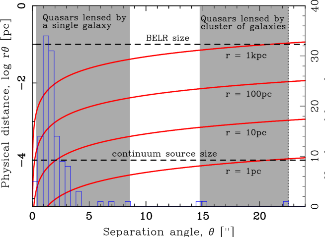
Figure 4: Physical distance between two sightlines of lensed images as a function of separation angle (red curves), adopting the absorber’s distance of $r$ = 1, 10, 100, and 1000 pc. The horizontal dotted lines mark sizes of BELR ($\sim$0.1 pc) and the continuum source ($\sim$10^-4 pc) of SDSS J1029+2623. The histogram denotes the distribution of separation angles of 124 lensed quasars that have been discovered to date. Shaded regions are ranges of separation angles of quasar images lensed by a single galaxy or by a cluster of galaxies.

References

- Balsara & Krolik (1993) Balsara, D. S., & Krolik, J. H. 1993, ApJ, 402, 109
- Blandford & Payne (1982) Blandford, R. D., & Payne, D. G. 1982, MNRAS, 199, 883
- Capellupo et al. (2013) Capellupo, D. M., Hamann, F., Shields, J. C., Halpern, J. P., & Barlow, T. A. 2013, MNRAS, 429, 1872
- Chartas et al. (2007) Chartas, G., Eracleous, M., Dai, X., Agol, E., & Gallagher, S. 2007, ApJ, 661, 678
- Chelouche & Netzer (2005) Chelouche, D., & Netzer, H. 2005, ApJ, 625, 95
- Chelouche (2003) Chelouche, D. 2003, ApJ, 596, L43
- Crotts & Fang (1998) Crotts, A. P. S., & Fang, Y. 1998, ApJ, 502, 16
- Dahle et al. (2013) Dahle, H., Gladders, M. D., Sharon, K., et al. 2013, ApJ, 773, 146
- de Kool & Begelman (1995) de Kool, M., & Begelman, M. C. 1995, ApJ, 455, 448
- Elvis (2000) Elvis, M. 2000, ApJ, 545, 63
- Everett (2005) Everett, J. E., 2005, ApJ, 631, 689
- Fohlmeister et al. (2013) Fohlmeister, J., Kochanek, C. S., Falco, E. E., et al. 2013, ApJ, 764, 186
- Gabel et al. (2006) Gabel, J. R., Arav, N., & Kim, T.-S. 2006, ApJ, 646, 742
- Ganguly et al. (2001) Ganguly, R., Bond, N. A., Charlton, J. C., Eracleous, M., Brandt, W. N., & Churchill, C. W., 2001, ApJ, 549, 133
- Gibson et al. (2008) Gibson, R. R., Brandt, W. N., Schneider, D. P., & Gallagher, S. C. 2008, ApJ, 675, 985
- Green (2006) Green, P. J. 2006, ApJ, 644, 733
- Hamann et al. (2013) Hamann, F., Chartas, G., McGraw, S., et al. 2013, MNRAS, 435, 133
- Hamann et al. (2012) Hamann, F., Simon, L., Hidalgo, P. R., & Capellupo, D. 2012, AGN Winds in Charleston, 460, 47
- Hamann et al. (2011) Hamann, F., Kanekar, N., Prochaska, J. X., et al. 2011, MNRAS, 410, 1957
- Hamann et al. (2008) Hamann, F., Kaplan, K. F., Rodríguez Hidalgo, P., Prochaska, J. X., & Herbert-Fort, S. 2008, MNRAS, 391, L39
- Hamann (1997) Hamann, F. 1997, ApJS, 109, 279
- Hamann et al. (1997a) Hamann, F., Barlow, T. A., Junkkarinen, V., & Burbidge, E. M., 1997, ApJ, 478, 80
- Inada et al. (2006) Inada, N., Oguri, M., Morokuma, T., et al. 2006, ApJ, 653, L97
- Inada et al. (2003) Inada, N., Oguri, M., Pindor, B., et al. 2003, Nature, 426, 810
- Joshi et al. (2014) Joshi, R., Chand, H., Srianand, R., & Majumdar, J. 2014, MNRAS, 442, 862
- Kaspi et al. (2000) Kaspi, S., Smith, P. S., Netzer, H., et al. 2000, ApJ, 533, 631
- Konigl & Kartje (1994) Konigl, A., & Kartje, J. F. 1994, ApJ, 434, 446
- Krolik & Kriss (2001) Krolik, J. H., & Kriss, G. A. 2001, ApJ, 561, 684
- Kurosawa & Proga (2009) Kurosawa, R. & Proga, D. 2009, ApJ, 693, 1929
- Lamy & Hutsemékers (2004) Lamy, H., & Hutsemékers, D. 2004, A&A, 427, 107
- Lopez et al. (2005) Lopez, S., Reimers, D., Gregg, M. D., et al. 2005, ApJ, 626, 767
- McLure & Dunlop (2004) McLure, R. J., & Dunlop, J. S. 2004, MNRAS, 352, 1390
- Misawa et al. (2014) Misawa, T., Charlton, J. C., & Eracleous, M. 2014, ApJ, 792, 77
- Misawa et al. (2013) Misawa, T., Inada, N., Ohsuga, K., et al. 2013, AJ, 145, 48
- Misawa et al. (2007a) Misawa, T., Charlton, J. C., Eracleous, M., et al. 2007a, ApJS, 171, 1
- Misawa et al. (2007b) Misawa, T., Eracleous, M., Charlton, J. C., & Kashikawa, N. 2007b, ApJ, 660, 152
- Murray et al. (1995) Murray, N., Chiang, J., Grossman, S. A., & Voit, G. M., 1995, ApJ, 451, 498
- Narayanan et al. (2004) Narayanan, D., Hamann, F., Barlow, T., Burbidge, E. M., Cohen, R. D., Junkkaribeb, V., & Lyons, R., 2004, ApJ, 601, 715
- Oguri et al. (2008) Oguri, M., Ofek, E. O., Inada, N., et al. 2008, ApJ, 676, L1
- Proga, Stone, & Kallman (2000) Proga, D., Stone, J. M., & Kallman, T. R., 2000, ApJ, 543, 686
- Rauch et al. (1999) Rauch, M., Sargent, W. L. W., & Barlow, T. A. 1999, ApJ, 515, 500
- Springel, Di Matteo, & Hernquist (2005) Springel, V., Di Matteo, T., & Hernquist, L. 2005, ApJ, 620, L79
- Takeuchi et al. (2013) Takeuchi, S., Ohsuga, K., & Mineshige, S. 2013, PASJ, 65, 88
- Trevese et al. (2013) Trevese, D., Saturni, F. G., Vagnetti, F., et al. 2013, A&A, 557, A91
- Tytler & Fan (1992) Tytler, D., & Fan, X.-M. 1992, ApJS, 79, 1
- Wise et al. (2004) Wise, J. H., Eracleous, M., Charlton, J. C., & Ganguly, R., 2004, ApJ, 613, 20