Stretching of BDT-gold molecular junctions: thiol or thiolate termination?

Amaury de Melo Souza,^a Ivan Rungger,^a Renato Borges Pontes,^b Alexandre Reily Rocha,^c Antonio Jose Roque da Silva,^d∗ Udo Schwingenschloegl,^e and Stefano Sanvito^a

Received Xth XXXXXXXXXX 20XX, Accepted Xth XXXXXXXXX 20XX
First published on the web Xth XXXXXXXXXX 200X

DOI: 10.1039/b000000x

It is often assumed that the hydrogen atoms in the thiol groups of a benzene-1,4-dithiol dissociate when Au-benzene-1,4-dithiol-Au junctions are formed. We demonstrate, by stability and transport properties calculations, that this assumption can not be made. We show that the dissociative adsorption of methanethiol and benzene-1,4-dithiol molecules on a flat Au(111) surface is energetically unfavorable and that the activation barrier for this reaction is as high as 1 eV. For the molecule in the junction, our results show, for all electrode geometries studied, that the thiol junctions are energetically more stable than their thiolate counterparts. Due to the fact that density functional theory (DFT) within the local density approximation (LDA) underestimates the energy difference between the lowest unoccupied molecular orbital and the highest occupied molecular orbital by several electron-volts, and that it does not capture the renormalization of the energy levels due to the image charge effect, the conductance of the Au-benzene-1,4-dithiol-Au junctions is overestimated. After taking into account corrections due to image charge effects by means of constrained-DFT calculations and electrostatic classical models, we apply a scissor operator to correct the DFT energy levels positions, and calculate the transport properties of the thiol and thiolate molecular junctions as a function of the electrodes separation. For the thiol junctions, we show that the conductance decreases as the electrodes separation increases, whereas the opposite trend is found for the thiolate junctions. Both behaviors have been observed in experiments, therefore pointing to the possible coexistence of both thiol and thiolate junctions. Moreover, the corrected conductance values, for both thiol and thiolate, are up to two orders of magnitude smaller than those calculated with DFT-LDA. This brings the theoretical results in quantitatively good agreement with experimental data.

1 Introduction

A long standing problem in the area of molecular electronics has been the difficulty of finding quantitative agreement between theory and experiment in some cases. This makes it difficult to design and build functioning devices based on molecules. More than a decade has passed since the pioneering experiment by Reed et al.,¹ and yet the well-known prototype molecular junction that consists of a benzene-1,4-dithiol molecule between two gold electrodes is still not fully understood. Numerous experimental ^{2, 3, 4, 5, 6, 7, 8, 7, 9} and theoretical ^{10, 11, 12, 13, 14, 15, 16} works have been reported, with both experimental and theoretical results varying over a large range.

In general, the possible experimental setups can be divided into two main categories: mechanically controlled break-junctions (MCBJs) ^{1, 8, 17, 9, 6, 18, 4, 3, 2, 19} and scanning tunneling microscopy (STM) experiments.^{20, 21, 22, 7, 23, 24, 25, 26, 27, 28, 5, 29} In the former, a gold nano-contact is created by stretching a gold wire and, just before rupture, a solution containing the target molecules is added to the system. Subsequently, the metallic contact is further stretched until rupture and in some cases the molecules remain trapped between the Au-Au tips forming the molecular junctions. In the second setup, the target molecules are deposited on a gold surface, and a STM tip is brought into contact to form the junction. Due to the nature of the experiment, several different geometrical contacts can be accessed during the stretching process of the junction, which leads to a statistical character of the experimental analysis. In fact, in a single experiment, a broad range of values of conductance, $G$, is observed, and possibly even very different average $G$ values between experiments.^{2, 9, 12} Yet, recent independent measurements ^{5, 22, 24, 19} agree on an average value of $G$ of about 0.01$G_{0}$, where $G_{0}=2e^{2}/h$ is the quantum conductance ($e$ is the electron charge and $h$ is the Planck’s constant).

From the theoretical point of view, the quantitative description of such molecular junctions is challenging for two main reasons. Firstly, realistic electrode configurations and many arrangements should be considered in the calculations, which becomes prohibitive within a fully ab initio approach. More recently, French et al. ^{15, 16} have applied a sophisticated method that combines Monte Carlo simulations and classical molecular dynamics to simulate the junction stretching process, allowing the sampling of hundreds of contact geometries between the molecule and the electrodes. In addition, it is generally assumed in the literature ^{30, 31, 32, 33, 15, 16, 34, 11, 12, 35, 14, 13, 36} that when the molecule attaches to the gold electrodes, the hydrogen atoms linked to the thiol groups are dissociated to form a thiolate-Au bond. However, recent DFT calculations on the details of the adsorption of the benzene-1,4-dithiol on gold have been reported.^{37, 38} They find that the thiol-Au structure is energetically more stable than its thiolate-Au counterparts when the molecule binds to either a perfect flat surface ³⁷ or to an adatom structure.³⁸

Usually transport calculations rely on the Kohn-Sham (KS) eigenvalues to evaluate $G$, even though these eigenvalues can not be rigorously interpreted as quasi-particle energy levels. The only exception is for the HOMO level, which is equal to the negative of the ionization potential.^{39, 40, 41} It has been demonstrated experimentally ^{42, 43, 44, 45, 46} that the quasi-particle energy gap, $E_{\mathrm{QP}}^{\mathrm{gap}}$, of a molecule, defined as the difference between its ionization potential, $I$, and electron affinity, $A$, shrinks with respect to that of the gas phase by adsorbing the molecule on a polarizable substrate. Nevertheless, the electronic structure theories usually used for such calculations can only partly account for this renormalization of the molecular energy levels when the junction is formed. It is well-known that DFT, within the standard local and semi-local approximations to the exchange-correlation (XC) energy, does not include non-local correlation effects, such as the dynamical response of the electron system to adding electrons or holes to the molecule. This limits its ability to predict the energy level alignment, when compared to experiments, which often leads to overestimated values for $G$.^{47, 48}

A rigorous way to include such non-local correlation effects is by using many-body perturbation theory, such as for example the GW approximation constructed on top of DFT.^{49, 50, 51} In the last few years, this approach has been used for evaluating level alignments,^{52, 53, 54, 55, 56, 57} in general with good success. The drawback of the GW scheme lays on the fact that it is highly computationally demanding, which limits the system size that can be tackled. This is particularly critical in the case of molecular junctions, where the system can be considerably large due to the presence of the metal electrodes. Therefore, different alternative approaches and corrections have been proposed to improve the description of the energy level alignment, for instance, corrections for self-interaction (SI) errors,^{13, 58} scissor operator (SCO) schemes ^{59, 35, 52, 48, 60} and constrained-DFT (CDFT).⁶¹

In the present work we investigate, by means of total energy DFT and quantum transport calculations, the stability and conductivity of thiol and thiolate molecular junctions. We compare the results for the two systems and we relate them to experimental data. The paper is divided as follows. In Sec. 2 we first give an overview of the methodology used. In Sec. 3.1 we present a systematic study of the adsorption process of two thiol-terminated molecules, namely, methanethiol and benzene-1,4-dithiol on Au(111) flat surface. For the latter, we also compare the stability of the thiol and thiolate systems when the junction is formed for several contact geometries.^{11, 12, 13, 15, 16} In Sec. 3.2 we discuss the energy level alignment, and present three methods used to correct the DFT-LDA molecular energy levels, namely CDFT and SCO. Based on these results in Sec. 3.3 we finally discuss the transport properties and present the dependence of $G$ on the electrodes separation ($L$) for flat-flat contact geometries, for both the thiol and thiolate junctions.

2 METHODS

2.1 Calculation details

All the calculations presented in this paper are based on DFT as implemented in the siesta package.⁶² For some calculations, we also use the plane-wave code vasp ⁶³ in order to compare with our results obtained with the localized basis set. Unless stated otherwise, we use the following parameters throughout this work. For total energy and relaxation calculations we use the generalized gradient approximation as formulated by Perdew-Burke-Ernzenhof (GGA-PBE) to the XC energy.⁶⁴ The basis set for siesta is the double-$\zeta$ polarized for carbon, sulfur and hydrogen and a double-$\zeta$ for the 5$d$6$s$6$p$ orbitals of Au atoms. We take into account corrections for the basis set superposition error (BSSE). The mesh cutoff is 300 Ry, four $k$-points are used for the Brillouin zone sampling in the perpendicular direction to the transport and norm-conserving pseudopotentials according to the Troullier-Martins procedure to describe the core electrons.⁶⁵ In the case of vasp calculations, we use a cut-off energy of 450 Ry to expand the wave functions and the projector augmented-wave method to treat the core electrons.⁶⁶ All the junctions are fully relaxed until all the forces are smaller than 0.02 eV/Å. All the quantum transport calculations presented are performed with the smeagol code,^{68, 67} which uses the non-equilibrium Green’s function (NEGF) formalism. Here, the XC energy is treated within the LDA approximation.

2.2 Self-interaction correction

One of the main deficiencies of local and semi-local DFT functionals when treating organic/inorganic interfaces is the SI error. This spurious interaction of an electron with the Hartree and XC potentials generated by itself leads to an over-delocalization of the electronic charge density. Consequently, the occupied KS eigenstates of molecules are pushed to higher energies. Moreover, the unoccupied states are found too low in energy due to the lack of the derivative discontinuity in the XC potential.⁴⁰ These two limitations lead to a substantial underestimation of the energy gap of various systems. In order to deal with the problem of SI, we apply the atomic self-interaction correction (ASIC) method,^{13, 69, 70, 58} which has been shown to improve the position of the highest occupied molecular orbital (HOMO) of molecules when compared to their gas phase $I$. It has also been shown to improve the energy level alignment when the junction is formed, leading to values of $G$ in better agreement with experiments.^{12, 13, 15, 16} The method, however, shows some limitations. The correction applied by ASIC depends on the atomic orbital occupation, not the molecular orbital occupation. Therefore, if different molecular orbitals are composed of a linear combination of a similar set of atomic orbitals, ASIC will shift their energy eigenvalues by a similar amount. For example, if empty states share the same character as the occupied states, as it is usually the case for small molecules, the energy of these states will be spuriously shifted to lower energies. In order to apply ASIC, a scaling parameter, $\alpha$, to the atomic-like occupations needs to be specified, where for $\alpha=1$ the full correction is applied, while for $\alpha=0$ no correction is applied. The value of $\alpha$ is related to the screening provided by the chemical environment.⁵⁸ For metals, where the SI is negligible, we therefore use $\alpha$=0, whereas for the molecules, where SI is more pronounced, we use $\alpha$=1.

2.3 Constrained Density Functional Theory

In the present work we apply the CDFT method, described in Ref. [ 61], to calculate the charge-transfer energy between the molecule and the metallic substrate. This corresponds to the position of the frontier energy levels, i.e., the HOMO and the lowest unoccupied molecular orbital (LUMO), with respect to the metal Fermi energy, $E_{\mathrm{F}}$. For a given distance, $d$, from the center of the molecule to the surface, the procedure is as follows: first, a conventional DFT calculation is performed, where no constraint is applied. This yields the total energy of the combined system, $E(\mathrm{mol}/\mathrm{sub};d)$, and the amount of charge present on each fragment (one fragment being the molecule and the other fragment the metal surface). In a second step, a CDFT calculation is performed. Since we are interested in accessing the position of the frontier energy levels with respect to the metal $E_{\mathrm{F}}$, we consider two types of constraints. In the first one, a full electron is removed from the molecule and added to the substrate, and the total energy of this charge-transfer state, $E(\mathrm{mol}^{+}/\mathrm{sub}^{-};d)$, is obtained. Hence, the energy to transfer one electron from the molecule to the substrate is given by

$$E_{\mathrm{CT}}^{+}(d)=E(\mathrm{mol}^{+}/\mathrm{sub}^{-};d)-E(\mathrm{mol}/\mathrm{sub};d)\>.$$ (1)

In the second case we evaluate the energy when one full electron is removed from the substrate and added to the molecule, $E(\mathrm{mol}^{-}/\mathrm{sub}^{+};d)$. The charge-transfer energy to add one electron to the molecule is then given by

$$E_{\mathrm{CT}}^{-}(d)=E(\mathrm{mol}/\mathrm{sub};d)-E(\mathrm{mol}^{-}/\mathrm{sub}^{+};d)\>.$$ (2)

We can relate the charge-transfer energies to the frontier energy levels by offsetting them with the metal work function ($W_{\mathrm{F}}$), so that $E_{\mathrm{HOMO}}(d)\simeq-[E^{+}_{\mathrm{CT}}(d)+W_{\mathrm{F}}]$ and $E_{\mathrm{LUMO}}(d)\simeq-[E^{-}_{\mathrm{CT}}(d)+W_{\mathrm{F}}]$ correspond to the HOMO and LUMO energies, respectively. Note that if the metal substrate is semi-infinite in size, then these relations are exact, since by definition the energy required to remove an electron from the metal and that gained by adding it are equal to $W_{\mathrm{F}}$. However, in a practical calculation a finite size slab is used, and therefore, the relations are only approximately valid due to the inaccuracies in the calculated $W_{\mathrm{F}}$ for finite systems. $W_{\mathrm{F}}$ is calculated by performing a simulation for the metal slab and by taking the difference between the vacuum potential and the $E_{\mathrm{F}}$ of the slab.

We can then compare the CDFT results for the renormalization of the energy levels due to the image charge effect with two simplified classical electrostatic models. In the first one we consider the electrostatic energy of a point charge interacting with a single surface,⁷¹ given by

$$V(d)=-\frac{q^{2}}{4(d-d_{0})}\>.$$ (3)

In the second model, the point charge is interacting with two infinite flat surfaces,^{59, 60} which gives the following interaction energy

$$U(d)=-\frac{q^{2}}{2(d-d_{0})}\mathrm{ln2}.$$ (4)

In both equations, $q$ is a point charge located at the center of the molecule, and $d=L/2$ for the case of two surfaces, where $L$ is the distance between the two surfaces; $d_{0}$ is the height of the image charge plane with respect to the surface atomic layer, so that $d_{0}$ can be interpreted as the center of gravity of the screening charge density formed on the metal surface, which in general depends on $d$. Instead of treating $d_{0}$ as a free parameter, as usually done in the literature,^{59, 60} our CDFT approach allows us to calculate it from first principles.⁶¹ Hence the classical models shown in Eq. (3) and Eq. (4) are effectively parameter-free when based on the CDFT value for $d_{0}$.

2.4 Scissor Operator method

Since we obtain the energies of the HOMO and LUMO from CDFT total energies, we can shift the DFT eigenvalues to lie at these energies by means of a SCO ^{72, 73, 60, 59, 74, 75} method. This has been shown to improve $G$ when compared to experimental data.⁵⁹ For the particular case of a single molecule attached to the electrodes, first a projection of the full KS-Hamiltonian matrix and of the overlap matrix is carried out onto the atomic orbitals associated with the molecule subspace, which we denote as $H_{\mathrm{mol}}^{0}$ and $S_{\mathrm{mol}}^{0}$ (the remaining part of $\hat{H}$ describes the electrodes). By solving the corresponding eigenvalue problem, $H_{\mathrm{mol}}^{0}\psi=\epsilon S_{\mathrm{mol}}^{0}\psi$, for this subblock we obtain the eigenvalues, $\{\epsilon_{n}\}_{n=1,...,M}$, and eigenvectors, $\{\psi_{n}\}_{n=1,...,M}$, where $M$ is the number of atomic orbitals on the molecule. Subsequently, the corrections are applied to the eigenvalues, where all the occupied levels are shifted rigidly by the constant $\Sigma_{\mathrm{o}}$ while the unoccupied levels are shifted rigidly by the constant $\Sigma_{\mathrm{u}}$. We note that in principle each state can be shifted by a different amount. Using the shifted eigenvalues we can construct a transformed molecular Hamiltonian matrix, $H_{\mathrm{mol}}^{\mathrm{SCO}}$, given by

$$H_{\mathrm{mol}}^{\mathrm{SCO}}=H_{\mathrm{mol}}^{0}+\Sigma_{\mathrm{o}}\sum_{i_{\mathrm{o}}=1,n_{\mathrm{o}}}\psi_{i_{\mathrm{o}}}\psi_{i_{\mathrm{o}}}^{\dagger}+\Sigma_{\mathrm{u}}\sum_{i_{\mathrm{u}}=1,n_{\mathrm{u}}}\psi_{i_{\mathrm{u}}}\psi_{i_{\mathrm{u}}}^{\dagger},$$ (5)

where the first sum runs over the $n_{\mathrm{o}}$ occupied orbitals, and the second one runs over the $n_{\mathrm{u}}$ empty states. In the full Hamiltonian matrix we then replace the subblock $H_{\mathrm{mol}}^{0}$ with $H_{\mathrm{mol}}^{\mathrm{SCO}}$.^{73, 60, 59, 74, 75} The SCO procedure can be applied self-consistently, although in this work we apply it non-selfconsistently to the converged DFT Hamiltonian.

The correction applied to the frontier energy levels of a molecule in a junction has two contributions. First we need to correct for the fact that the gas-phase LDA HOMO-LUMO gap ($E_{\mathrm{LDA}}^{\mathrm{gap}}$) is too small when compared to the difference between $I$ and $A$, where $I=E^{(N-1)}-E^{(N)}$ and $A=E^{(N)}-E^{(N+1)}$ ($E^{(N)}$ is the ground state total energy for a system with $N$ electrons). Secondly, the renormalization of the energy levels, when the molecule is brought close to metal surfaces needs to be added to the gas-phase HOMO and LUMO levels. Although CDFT in principle allows us to assess the renormalization of the energy levels in the junction, to reduce the computational costs we calculate the charge-transfer energies with one single surface. Since in transport calculations there are two surfaces, we then use the corresponding classical model (Eq. 4), with $d_{0}$ obtained from CDFT for the single surface. Hence, for the molecule attached to two metallic surfaces forming a molecular junction, we approximate the overall corrections for the molecular levels below $E_{\mathrm{F}}$ by

$$\Sigma_{\mathrm{o}}(d)=-[I+\epsilon_{\mathrm{HOMO}}(d)]+U(d)$$ (6)

and similarly for the levels above $E_{\mathrm{F}}$ as

$$\Sigma_{\mathrm{u}}(d)=-[A+\epsilon_{\mathrm{LUMO}}(d)]-U(d);$$ (7)

where $\epsilon_{\mathrm{HOMO/LUMO}}(d)$ is obtained from the position of the peaks of the PDOS and $U(d)$ is the classical potential given by Eq. (4). Here we assume a that the character of the molecular states is preserved when the junction is formed.

2.5 Electronic transport properties: DFT+NEGF

For the transport calculations, the system is divided into three regions: the central region, called scattering region or device (D) region, which includes the molecule and a few layers of both the electrodes, and the semi-infinite left (L) and right (R) electrodes, to which the device region is connected. The retarded Green’s function of the device region, $\mathcal{G}_{\mathrm{D}}$, is then given by

$$\mathcal{G}_{\mathrm{D}}(E)=\lim_{\eta\rightarrow 0}\left[(E+i\eta)-H_{\mathrm{D}}-\Sigma_{\mathrm{L}}-\Sigma_{\mathrm{R}}\right]^{-1},\\$$ (8)

where $\Sigma_{\mathrm{{L,R}}}$ are the so-called self-energies of the left-hand and right-hand side electrodes, $E$ is the energy and $H_{\mathrm{D}}$ is the KS-Hamiltonian of the central region. The electronic couplings between the electrodes and the device region are given by $\Gamma_{\mathrm{{L,R}}}=i(\Sigma_{\mathrm{{L,R}}}-\Sigma_{\mathrm{{L,R}}}^{\dagger})$. Following a self-consistent procedure,⁶⁸ the non-equilibrium charge density extracted from Eq. (8) is used to calculate a new $H_{\mathrm{D}}[\rho]$. Once the convergence is reached, the transmission coefficients are calculated as

$$T=\mathrm{Tr}[\mathrm{\Gamma_{\mathrm{L}}\mathcal{G}_{\mathrm{D}}^{\dagger}\Gamma_{\mathrm{R}}\mathcal{G}_{\mathrm{D}}}].$$ (9)

In the limit of zero-bias, we obtain the zero-bias conductance from the Fisher-Lee relation $G=G_{0}T(E_{\mathrm{F}})$ and the projected DOS (PDOS) for any orbital with index $\beta$ as

$$\mathrm{PDOS}_{\beta}(E)=\frac{1}{2\pi}\mathrm{Im}[\mathcal{G}_{\mathrm{D}}(E)S_{\mathrm{D}}]_{\beta\beta}.$$ (10)

In order to obtain reliable values for $T$ it is important to have an electronic structure theory capable of describing the correct positions of the molecular energy levels with respect to $E_{\mathrm{F}}$, since these ultimately dictate the transport properties of the device.

3 RESULTS

3.1 Stability study of thiol-terminated molecules on a Au(111) flat surface and the junctions

In this section we present a systematic study, by means of total energy DFT calculations, of the stability of thiol-terminated molecules on Au(111) flat surfaces, as well as when the molecule is attached to two Au electrodes forming a molecular junction. For the systems presented in this section, the gold surface is modeled by considering a 3$\times$3 surface unit cell five-layer thick. This corresponds to a surface coverage of 1/3.^{12, 37} The three bottom layers of gold are kept fixed during the relaxation. For the junctions shown in Fig. 3 we use a slightly larger 4$\times$4 surface unit cell, in order to be able to model the tip-tip-like contact as well.

We first discuss the adsorption process of benzene-1-4-dithiol ($\mathrm{C_{6}H_{6}S_{2}}$) on the Au(111) flat surface, and compare it to adsorption properties of methanethiol ($\mathrm{CH_{3}SH}$). These molecules represent two distinct classes, namely, aromatic and linear hydrocarbon compounds, respectively. From this point on, we refer to benzene-1-4-dithiol as BDT2H in order to distinguish it from the benzene-1-thiolate-4-thiol $\mathrm{C_{6}H_{5}S_{2}}$ (BDT1H), and from benzene-1-4-dithiolate $\mathrm{C_{6}H_{4}S_{2}}$ (BDT). The calculations are performed as follows: (i) a system with the molecule terminated by a thiol group ($R\mathrm{SH/Au}$), where $R=\mathrm{CH_{3}}$ for the methanethiol and $R=\mathrm{C_{6}H_{5}S}$ for the BDT2H, is placed close to the Au(111) surface and the geometry is relaxed. (ii) Then a second system is built where the molecule is now terminated by a thiolate group and a H atom is attached to the surface ($R\mathrm{S/Au+H}$), and again the geometry is relaxed. Fig. 1(a-c) shows the relaxed structures for the dissociative adsorption of the methanethiol molecule, and the analogous structures are shown for the BDT2H in Fig. 1(d-f). For the $R\mathrm{SH/Au}$ systems, the molecule is tilted with respect to its vertical axis perpendicular to the surface, whereas for the $R\mathrm{S/(Au+H)}$ systems the molecule is upright sitting on a hollow-site. Our relaxed geometries are in good agreement with literature.^{36, 37} We have also calculated the binding energies, as given by

$$E_{\mathrm{b}}=E_{\mathrm{T}}(R\mathrm{SH/Au})-E_{\mathrm{T}}(\mathrm{Au})-E_{\mathrm{T}}(R\mathrm{SH}),$$ (11)

for the methanethiol and methanethiolate molecules on the Au(111) surface, and we find 0.63 eV and 1.42 eV, respectively. For the BDT2H we find 0.12 eV whereas for the BDT1H, $E_{\mathrm{b}}$ is equal to 1.53 eV.

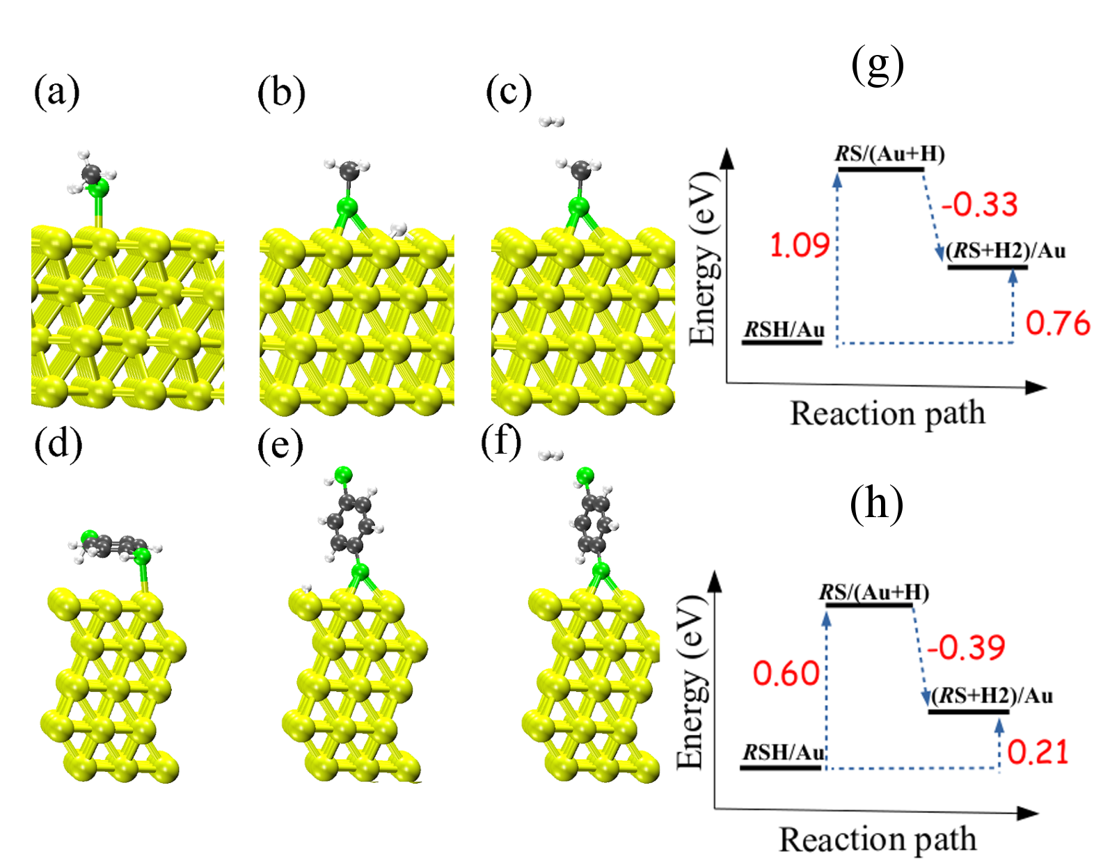
Fig.  1: Ball-stick representation of the adsorption process of methanethiol (a-c) and BDT2H (d-f) on a flat Au(111) surface. (a) and (d) the thiol molecules (RSH/Au) are adsorbed on the surface; (b) and (e) the hydrogen atom is dissociated to form thiolates (RS/(Au+H)). Finally, in (c) and (f) the hydrogen atoms attached to the Au surface desorbs to form a $H_{2}$ molecule ((RS+$H_{2}$)/Au). (g) and (h) schematically show the total energy differences between each step of the reaction.

Finally, we consider a third structure for which the H atom attached to the surface is released from the surface to form a $\mathrm{H_{2}}$ molecule $(R\mathrm{S+H_{2})/Au}$. The formation energy of the thiolate structure with a H atom attached to the surface is given by

$$E_{\mathrm{f}}=E_{\mathrm{T}}{(R\mathrm{SH/Au})}-E_{\mathrm{T}}{(R\mathrm{S/(Au+H)})}.$$ (12)

Similarly, the formation energy for the dissociative adsorption followed by the formation of a $\mathrm{H_{2}}$ molecule is calculated by

$$E_{\mathrm{f}}=E_{\mathrm{T}}{(R\mathrm{SH/Au})}+\frac{1}{2}E_{\mathrm{T}}(\mathrm{H_{2}})-E_{\mathrm{T}}((R\mathrm{S+H_{2})/Au}).$$ (13)

Fig. 1(g) and Fig. 1(h) schematically show the total energy differences between each step of the dissociative adsorption of the methanethiol and BDT2H molecules. For the methanethiol molecule, if the dissociative reaction is accompanied by the chemisorption of a H atom on the surface, as in Fig. 1(b), the thiolate structure is energetically unfavorable by 1.09 eV, a result consistent with previous calculations by Zhou et al. ⁷⁶ and temperature-programmed desorption (TPD) experiments.^{77, 78} When the H atoms adsorbed on the surface are detached to form $\mathrm{H_{2}}$ molecules as in Fig. 1(c), the thiolate system becomes more stable by 0.33 eV compared to the thiolate system with the H atom attached to the surface. Overall, the dissociative reaction followed by the formation of a $\mathrm{H_{2}}$ molecule is unfavorable by 0.76 eV. For the BDT2H molecule, the thiolate with a H atom attached to the surface is unfavorable by 0.60 eV compared to the thiol structure, in good agreement with the value of 0.4 eV reported in recent studies by Ning et al..³⁸ When the dissociative reaction is accompanied by the formation of a $\mathrm{H_{2}}$ from the H atom attached to the surface, this reaction is exothermic by 0.39 eV. As a result, the dissociative absorption of BDT2H molecules on Au(111) surface followed by the desorption of $\mathrm{H_{2}}$ is unfavorable by 0.21 eV. This partially contradicts the results obtained by Nara et al.,³⁷ who found the dissociative reaction accompanied by the H atom on the surface to be indeed unfavorable by 0.22 eV. However, for the case where the reaction is followed by the formation of $\mathrm{H_{2}}$, the system is further stabilized by 0.42 eV so that the thiolate system is more stable by $\sim$0.20 eV. Overall our results show that for both classes of molecules the dissociative reaction is always unfavorable when considering either the formation of $R\mathrm{S/(Au+H)}$ or $(R\mathrm{S+H_{2})/Au}$ structures.

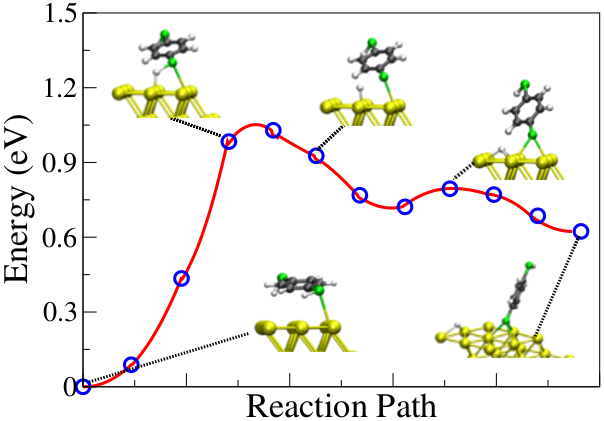
Fig.  2: Activation barrier for the dissociative adsorption of BDT2H on Au(111) surface as shown in Fig. 1(d)-(e).

In addition to the total energy differences between the dissociated and non-dissociated structures of BDT2H, we evaluate the barrier height between those states [Fig. 1(d) and Fig. 1(e)], by means of the Nudged Elastic Band (NEB) method,^{79, 80, 81} as shown in Fig. 2. This allows us to estimate the transition probability between the states. Our results show that the activation barrier is about 1 eV. The fact that the barrier is large provides evidence for possible existence of the thiol structures on the surface, since a high temperature is required to overcome such a barrier. We note that defects on the surface, such as adatom, or the presence of a solvent, can change the energy barrier and eventually dissociation might take place at lower energies.

For the BDT2H molecule we also compare the stability of the thiol and thiolate structures when the molecule is connected to two Au electrodes. We consider three types of junctions, as illustrated in Fig. 3.

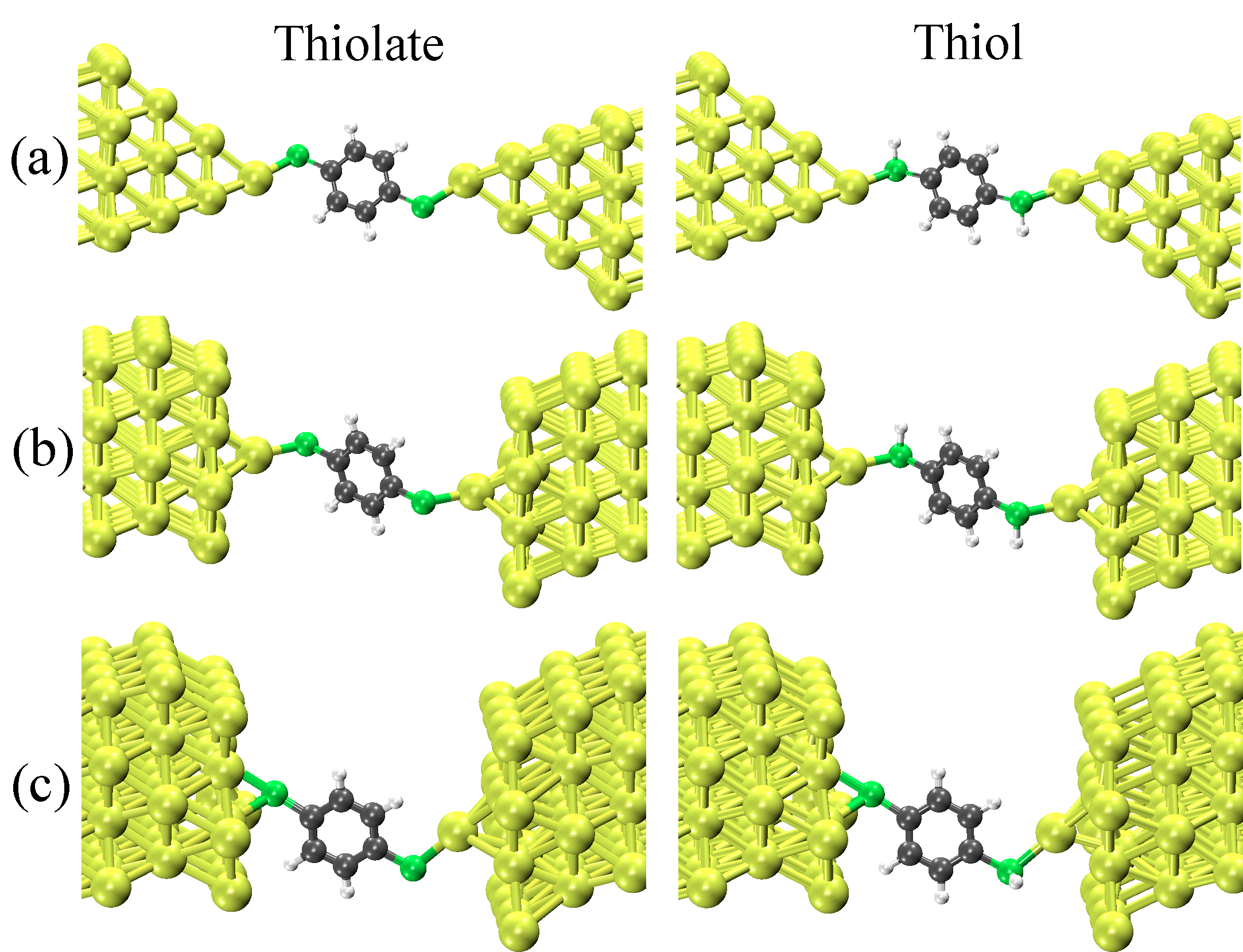
Fig.  3: Ball-stick representation of three molecule-electrode contact geometries. (a), (b) and (c) shows the tip-tip, adatom-adatom and surface-adatom configurations, respectively. Left (right) panel shows the thiolate (thiol) junctions.

For the configuration shown in Fig. 3(a), ten gold atoms are added on each side of the junction forming a tip-like symmetric contact with the molecule. For the configuration shown in Fig. 3(b), an adatom is added symmetrically on each side of the junction and for the one shown in Fig. 3(c), an adatom is added to one side of the junction and the molecule is connected to a flat surface on the other side. These junctions constitute typical models for transport calculations found in the literature.^{13, 14, 54} In this case, the formation energy difference between the thiol and the thiolate structures with respect to the formation of $\mathrm{H_{2}}$ molecule is given by

$$E_{\mathrm{f}}=E_{\mathrm{T}}(\mathrm{BDT2H/Au})-E_{\mathrm{T}}(\mathrm{BDT/Au})-E_{\mathrm{T}}(\mathrm{H_{2}}),$$ (14)

and the results are shown in Table. 1. Note that for the adatom-flat configuration the binding energy is evaluated considering $\frac{1}{2}\mathrm{H_{2}}$. For all the three junctions, the thiol configurations are energetically more stable than their thiolate counterparts.

Table 1: Formation energy difference between the thiol and the thiolate structures with respect to the formation of $\mathrm{H_{2}}$ molecule, in eV, for the three molecular junctions shown in Fig. 3.

System	VASP	SIESTA
surface-adatom	-0.36	-0.42
adatom-adatom	-0.64	-0.40
tip-tip	-0.77	-0.88

One possibility that has been considered in order to determine whether there are thiols or thiolates in the junction is a simultaneous measurement of $G$ and force in a STM and atomic force microscopy (AFM) setup.^{82, 83, 84, 85} Since the binding energy for thiol and thiolate can differ considerably, one might expect that the forces involved when stretching the junction should be different. Therefore, we investigate the energetics of Au(111)-BDT-Au(111) and Au(111)-BDT2H-Au(111) junctions as a function of $L$. For the Au(111)-BDT-Au(111) junctions, similar calculations have been reported in the literature in on attempt to simulate a MCBJ experiment within DFT.^{12, 15, 16, 86, 87, 88, 89} Details on how the stretching is performed can be found in Ref. [ 12]. Figs. 4(a)-(i) and Figs. 5(a)-(i) show the relaxed structures for the Au(111)-BDT-Au(111) and Au(111)-BDT2H-Au(111) junctions undergoing stretching.

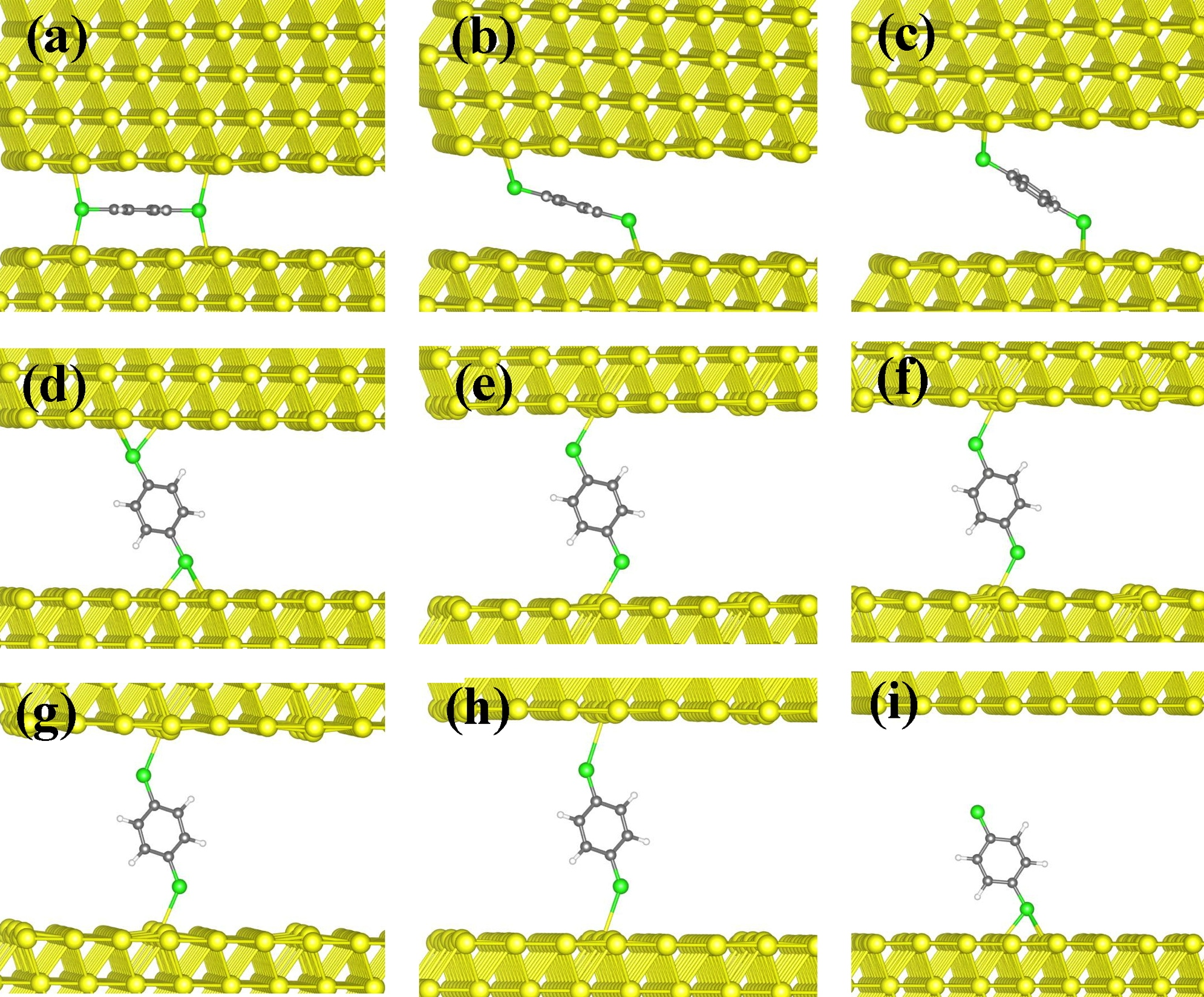
Fig.  4: (a)-(i) Ball-stick representation of the stretching process of BDT between two flat surfaces.

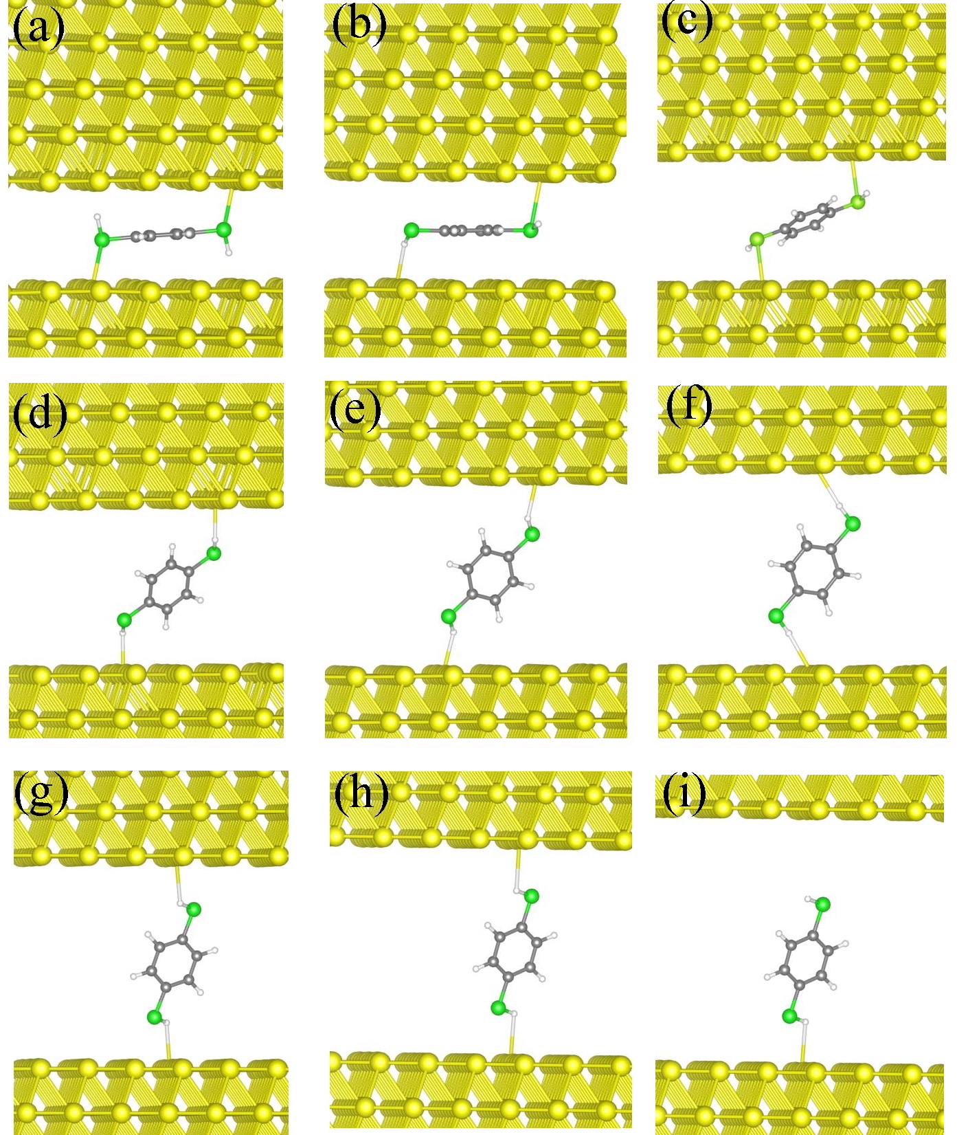
Fig.  5: (a)-(i) Ball-stick representation of the stretching process of BDT2H between two flat surfaces.

In Fig. 6 we show the energy and the forces as a function of $L$, for both Au(111)-BDT-Au(111) and Au(111)-BDT2H-Au(111) junctions. Our results show that the breaking force for the S-Au bond is about 1 nN, in good agreement with independent DFT results by Romaner et al. ⁸⁷ of 1.25 nN obtained using the same contact geometry. The authors also considered the scenario when the BDT molecule is attached to an adatom contact geometry, and they found that the breaking force can be as large as 1.9 nN.⁸⁷ In fact, it is possible that during the elongation process the molecule is bonded to a single Au atom rather than a flat surface.¹⁵ For Au(111)-BDT2H-Au(111) our calculated breaking force is  0.3 nN, as shown in Fig. 6(b). Thus the breaking forces for the BDT2H junctions are smaller than for those of BDT when the flat electrode geometry is considered. We note that this is much smaller than the calculated value of 1.1-1.6 nN for the BDT2H molecule attached to a tip-like contact geometry.³⁸ Our small value of breaking forces of  0.3 nN for the thiol junctions is consistent with the rather small calculated $E_{\mathrm{b}}$ of 0.12 eV, and indicates weak coupling between the molecule and the flat electrodes. A similar study for a octanedithiol-Au junction has also been reported,⁸⁹ and for an asymmetric junction they found the breaking force of the Au-thiol bond to be 0.4-0.8 nN. Other experiments using the same molecule ^{84, 85} reported a breaking force of  1.5 nN, which is very similar to the breaking force of a Au-Au bond, therefore, leading to the conclusion that the junction might break at the Au-Au bond and also indicating the presence of Au-thiolate instead of Au-thiol junctions.

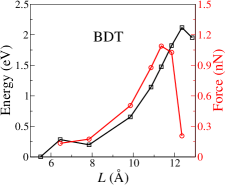
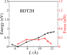
Fig.  6: Total energy and pulling force as a function of $L$ for the Au-BDT-Au and Au-BDT2H-Au molecular junctions shown in Fig. 4 and Fig. 5, respectively.

In summary, we find that the dissociative reaction of methanethiol and BDT2H on Au(111) is energetically unfavorable. Especially for the BDT2H, the activation barrier of $\sim$1 eV strongly suggests the presence of thiol structures when the molecules attach to the metallic surface. Moreover, for all the contact geometries of molecular junctions presented in Figs. 3-5, the thiol systems are also energetically more stable. These results indicate that the non-dissociated structures are likely to exist in experiments, and therefore should be considered when modeling transport properties of such systems.

3.2 Energy level alignment

One of the possible reasons for the discrepancies between theory and experiments regarding the conductance of molecular junctions is the difficulty, from a theoretical point of view, to obtain the correct energy level alignment of such systems. Table. 2 shows the LDA eigenvalues for the frontier molecular states of BDT and BDT2H in the gas phase. $E_{\mathrm{LDA}}^{\mathrm{gap}}$ is largely underestimated when compared to $E_{\mathrm{QP}}^{\mathrm{gap}}=I-A$ calculated by the so-called delta self-consistent field ($\Delta$SCF) method. For the BDT molecule, our results show that the HOMO is higher in energy by 2.73 eV with respect to $-I$ whereas the LUMO is lower in energy by 2.66 eV compared to $-A$. For the BDT2H, the HOMO is higher in energy by 2.49 eV with respect to $-I$, and the LUMO is lower in energy by 2.51 eV when compared to $-A$. The results clearly indicate that the KS eigenvalues offer a poor description of the molecule quasi-particle levels even in the gas phase within GGA/LDA.

Fig. 7(a) shows schematically the energies of these states for the gas phase molecules. In the case of BDT2H molecule, the wavefunctions $\Psi_{0}$ (blue), $\Psi_{1}$ (red) and $\Psi_{2}$ (green) correspond to the HOMO-1, HOMO and LUMO of the isolated molecule, respectively. For the BDT the removal of 2 H atoms when compared to BDT2H leads to a reduction of the number of electrons by 2 as well, so that to a first approximation the BDT2H HOMO becomes the LUMO for the BDT molecule [see Fig. 8(b) and 8(e)]. Therefore, for BDT, $\Psi_{0}$ corresponds to the HOMO, $\Psi_{1}$ to the LUMO, and $\Psi_{2}$ to the LUMO+1. Fig. 8 shows the real space representation of $\Psi_{0}$, $\Psi_{1}$ and $\Psi_{2}$ for BDT (left) and BDT2H (right) molecules in the gas phase.

Table 2: Calculated LDA eigenvalues ($\epsilon$), $E_{\mathrm{LDA}}^{\mathrm{gap}}$, $I$, $A$ and $E_{\mathrm{QP}}^{\mathrm{gap}}$ (calculated with $\Delta$SCF) for the gas phase BDT and BDT2H molecules.

	LDA				$\Delta$SCF
System	$\epsilon\mathrm{{}_{HOMO}}$	$\epsilon\mathrm{{}_{LUMO}}$	$E_{\mathrm{LDA}}^{\mathrm{gap}}$		-I	-A	$E_{\mathrm{QP}}^{\mathrm{gap}}$
BDT	-5.74	-5.19	0.55		-8.47	-2.53	5.94
BDT2H	-5.09	-1.82	3.27		-7.58	0.69	8.27

Fig. 7(b) shows the CDFT results for $E_{\mathrm{HOMO}}/E_{\mathrm{LUMO}}$ as a function of $d$ for the BDT/Au(111) system (see Sec. 2.3). In the CDFT calculations the metal is modeled by a 9$\times$9 Au(111) surface with five atomic layers and the molecule placed upright at a distance, $d$, from the center of the molecule to the Au surface, and we use a 20 Å vacuum region in the direction perpendicular to the surface plane. We note that although CDFT is in principle applicable at all $d$, when $d$ becomes less than about $5.9$ Å, for which the Au-S bond distance, $d_{\mathrm{Au-S}}$, is less than 2.5 Å, the amount of charge on each fragment is ill defined due to the hybridization between the molecular orbitals and the electrode continuum. Therefore, at those small distances, the CDFT charge-transfer energies are not well defined. At $d=5.9$ Å, the CDFT calculations give an overall reduction of $E_{\mathrm{QP}}^{\mathrm{gap}}$ of 2.09 eV with respect to the value obtained for isolated BDT.

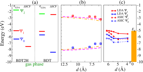
Fig.  7: Energy level alignment of the frontier molecular orbitals for the BDT molecule from the gas phase to the formation of the Au-BDT-Au junction. (a) LDA eigenvalues ($\epsilon_{\mathrm{LDA}}$) and $\Delta$SCF calculations in the gas phase BDT. For comparison, we also show results for the gas phase of BDT2H. All the values are given with respect to the vacuum level. (b) CDFT calculations for the charge-transfer energies between BDT molecule adsorbed and a single flat surface: $E_{\mathrm{CT}}^{+}(d)$ (blue squares) and $E_{\mathrm{CT}}^{-}(d)$ (red squares). The classical image charge contribution for two surfaces (dashed-line) and for a single surface (dashed-dotted line) are plotted for comparison where $E_{\mathrm{F}}=-5.1$ eV and $d_{0}=1$ Å. (c) LDA and ASIC energy levels for the HOMO ($\Psi_{0}$) and LUMO ($\Psi_{1}$) obtained from the PDOS peaks for the molecule at the junction as a function of $d=L/2$.

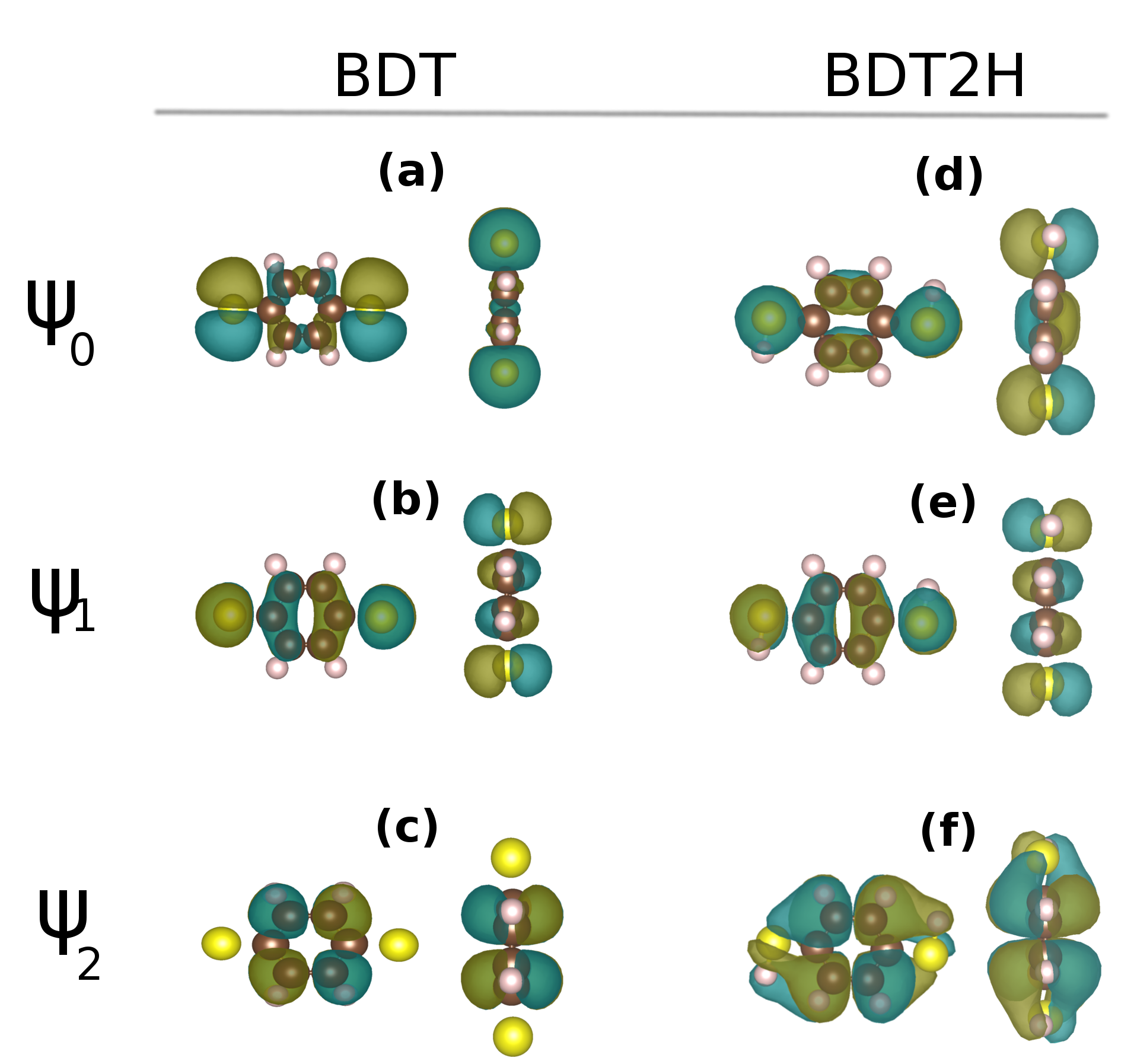
Fig.  8: Plots of wavefunctions: (a), (b) and (c) show $\Psi_{0}$ (20th state), $\Psi_{1}$ (21st state) and $\Psi_{2}$ (22sd state), respectively, for the gas phase BDT molecule; (d), (e) and (f) show the same for the the BDT2H molecule. Isosurfaces are taken at a density of 0.06 $e/\mathrm{\AA^{3}}$.

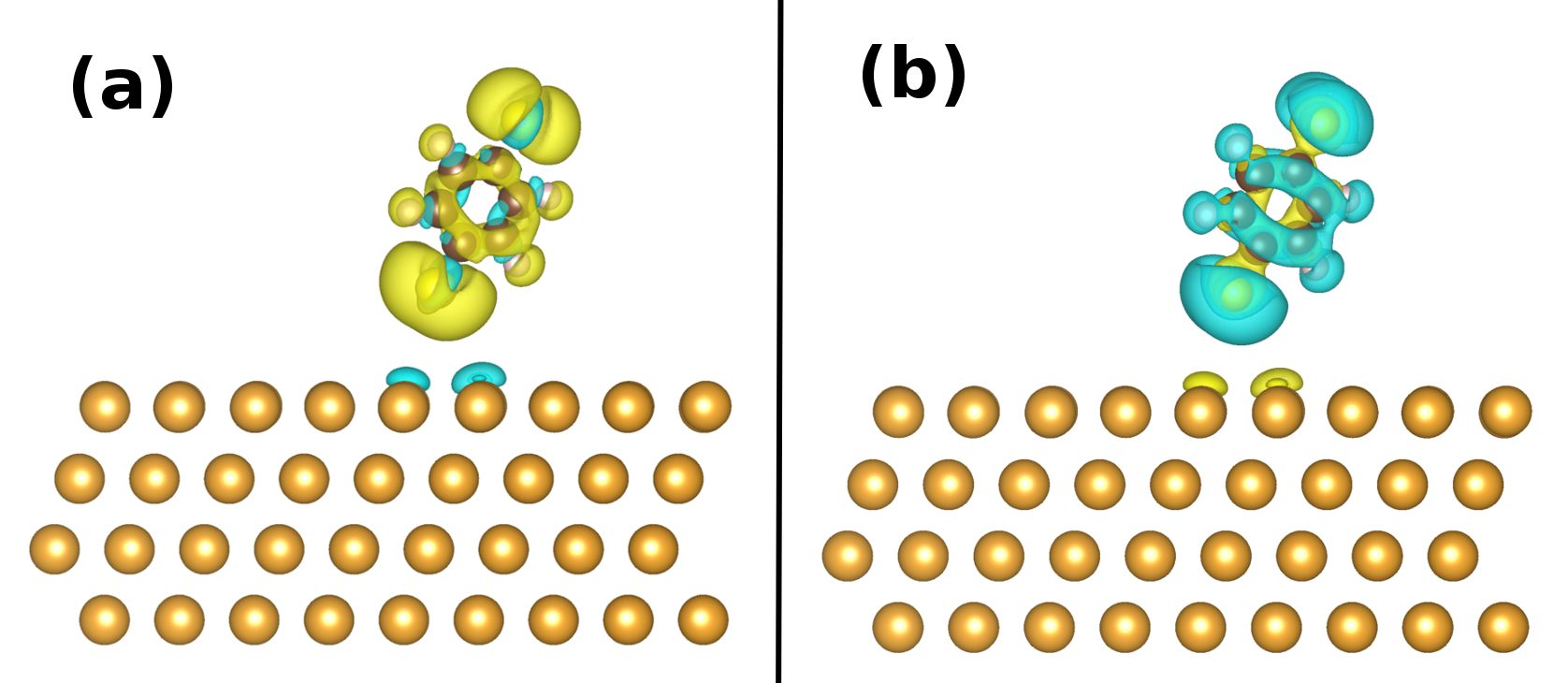
Fig.  9: Charge density differences for (a) $E_{\mathrm{CT}}^{+}(d)$ and (b) $E_{\mathrm{CT}}^{-}(d)$ for $d=6.9$ Å. Isosurfaces are taken at $10^{-4}\leavevmode\nobreak\ \mathrm{e/\AA^{3}}$.

Fig. 7(b) also shows the results of the classical model for the image charge calculated for one [Eq. (3), dashed line] and for two [Eq. (4), dash-dotted line] surfaces. The CDFT $d_{0}$ ranges from 0.79 Å to 1.13 Å, depending on the distance, and we therefore take $d_{0}=1$ Å as average value. Coincidentally, this is the same value used in literature,^{60, 73, 46} where it was however not formally justified, but rather used as a free parameter. The corrections to $I$ and $A$ from the classical model when considering two surfaces are larger than the corrections for a single surface, since $U(d)>V(d)$ for all $d$. We evaluate the charge density differences between the constrained and non-constrained calculations for $E_{\mathrm{CT}}^{+}(d)$ and $E_{\mathrm{CT}}^{-}(d)$ (Fig. 9). It can be seen that the hole (electron) left on the molecule has the same character as the corresponding $\Psi_{0}$ ($\Psi_{1}$) wavefunction [compare to Figs. 8(a)-(b)].

Fig. 7(c) shows the energies of the eigenvalues of the $\Psi_{0}$ and $\Psi_{1}$ states for the BDT molecule as a function of $d=L/2$, calculated with LDA (solid lines) and ASIC (dashed lines), for the stretching configurations shown in Fig. 4(c-h). The energies of these levels are set to be at the peaks of the corresponding PDOS. In the limit of weak coupling between the BDT molecule and the electrodes, which is the case for $L=12.35$ Å, at which $d_{\mathrm{Au-S}}$ is the largest before rupture of the junction, LDA gives the LUMO of the isolated BDT molecule ($\Psi_{1}$) slightly above $E_{\mathrm{F}}$. However, as shown in Fig. 7(a) and Table. 2, the corrected energy of $\Psi_{1}$ (which is given by $-A$) is 2.66 eV above the LDA eigenvalue. Similarly, the LDA energy of $\Psi_{0}$ is too high by 2.73 eV when compared to $-I$. The same analysis can be done for $L=11.86$ Å and $L=11.36$ Å, for which $\Psi_{1}$ is still above $E_{\mathrm{F}}$. In other words, for $L\geq 11.36$Å, the molecule is weakly bonded to the electrodes, therefore, charge transfer from the electrodes to the molecule due to the hybridization of the molecular and electrodes states is small. These results show that for the Au-BDT-Au junctions in the weak coupling regime the LDA BDT HOMO (corresponding to $\Psi_{0}$) is in fact too high in energy whereas the LDA BDT LUMO (corresponding to $\Psi_{1}$) is too low.

In order to correct the energy levels, we apply the SCO method (see Sec. 2.4). Table. 3 shows, for the Au-BDT2H-Au and Au-BDT-Au junctions, $U$ [Eq. (4)], $\Sigma_{\mathrm{o}}$ [Eq. (6)] and $\Sigma_{\mathrm{u}}$ [Eq. (7)] as functions of $L$. As pointed out by Garcia-Suarez et al.,⁶⁰ the shift of the energy level is unambiguous when there is no resonance at $E_{\mathrm{F}}$,^{59, 73} so that the occupied levels are shifted downwards and the empty levels are shifted upwards in energy. This is the case for the BDT2H molecule, where the isolated molecule has 42 electrons, therefore the 21st molecular level is the HOMO of the isolated molecule ($\Psi_{1}$ in this case). Since it is already filled with two electrons, it lies below $E_{\mathrm{F}}$ when the molecule is in the junction, and the LUMO ($\Psi_{2}$) is always empty and well above $E_{\mathrm{F}}$.

Table 3: Contribution due to the classical image charge for two surfaces model ($U$) and the final corrections $\Sigma_{\mathrm{o}}/\Sigma_{\mathrm{u}}$ as a function of $L$ for BDT2H and BDT molecules at the junction. The first column correspond to the labels of a subset of the structures shown in Fig. 4 and Fig. 5. The Au-S bond distance, $d_{\mathrm{Au-S}}$, is also shown for completeness.

						BDT2H			BDT
	$L$ (Å)	$d_{\mathrm{Au-S}}$ (Å)		U (eV)		$\Sigma_{\mathrm{o}}$(eV)	$\Sigma_{\mathrm{u}}$ (eV)		$\Sigma_{\mathrm{o}}$(eV)		$\Sigma_{\mathrm{u}}$ (eV)
(c)	7.86	2.11		1.70		0.18	1.63		-		-
(d)	9.89	2.08		1.26		-0.50	1.72		-		-
(e)	10.87	2.47		1.12		-0.80	1.78		-		-
(f)	11.36	2.67		1.06		-1.04	1.77		-1.13		1.45
(g)	11.84	2.90		1.01		-0.62	2.22		-1.63		1.53
(h)	12.35	3.18		0.96		-0.83	2.17		-1.84		1.55

For closer distances, due to the stronger coupling between molecule and electrodes, hybridization occurs leading to a fractional charge transfer from the electrodes to the molecule. For small $d$ also for the BDT molecule the $\Psi_{1}$ state becomes partially occupied, and positioned slightly below $E_{\mathrm{F}}$. This means that, for the structures considered in Fig. 4, the correction defined by Eq. 7 can not be applied for $L\leq 10.87$, since this is the distance where the level moves slightly below $E_{\mathrm{F}}$. We note that when the level is pinned at $E_{\mathrm{F}}$, many-body effects become important, and the GW method might be the most appropriate approximation.³⁵ Once the coupling is strong enough, and $\Psi_{1}$ is almost fully filled, it becomes effectively the HOMO of the BDT. In this case we expect its energy to be too high within LDA, and therefore application of ASIC is expected to improve its position with respect to $E_{\mathrm{F}}$. In fact, ASIC corrects $\Psi_{1}$ by $\sim$1 eV as $d$ decreases, as shown in Fig. 7(c).

For the weak coupling limit the calculated corrections show that $\Psi_{1}$ (the LUMO of the isolated BDT molecule) is empty and its LDA eigenvalue is too low in energy. In contrast, for the strong coupling limit the energy of $\Psi_{1}$ moves below $E_{\mathrm{F}}$, so that the state becomes occupied, and its LDA eigenvalue is now too high in energy. In this regime we apply the ASIC method to give a better description of the energy level alignment.

3.3 Electronic Transport Properties: Thiol versus Thiolate Junctions

For the electronic transport properties, we start by presenting results for the molecular junctions at fixed distance and different molecule-surface bonding. Subsequently we discuss the conductivity of the thiol and thiolate systems attached to flat Au electrodes under stretching.

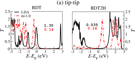
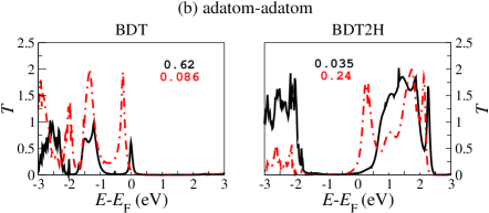
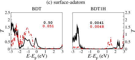
Fig.  10: (a) Transmission coefficients as a function of energy for thiolate (left column) and thiol (right column) for the structures shown in Fig. 3. For each case we report the transmission at $E_{\mathrm{F}}$ for both LDA (black full-line) and ASIC (red dashed-line) results.

Fig. 10 shows $T(E)$ for the thiolate (left column) and thiol (right column), for tip-tip, adatom-adatom and surface-adatom structures (see Fig. 3 for the structure geometries). Within the LDA functional, the transmission curves of all the thiolate junctions present a peak pinned at $E_{\mathrm{F}}$. These results have been found in several works reported in the literature for Au-BDT-Au (thiolate) junctions.^{13, 12, 35, 9, 15, 16} The resonant states at $E_{\mathrm{F}}$ yield high values of $G$ of 1.35$G_{0}$, 0.45$G_{0}$ and 0.22$G_{0}$ for tip-tip, surface-adatom and adatom-adatom, respectively. The observed peaks at $E_{\mathrm{F}}$ correspond to the hybridized $\Psi_{1}$ state of the BDT molecule. Note that the exact position of the peaks and so the exact $G$ values depend on the atomistic details of the junctions, as well as on the functionals used within DFT. We point out that such high values of $G$ have never been observed experimentally, indicating that LDA does not give the correct energy level alignment between the molecule and the electrodes, as already discussed in Sec. 3.2. In contrast, for the thiol junctions, no resonant states are found around $E_{\mathrm{F}}$. The zero-bias conductance is in the range of 0.035-0.004$G_{0}$, which is in good agreement with experimental values of 0.011$G_{0}$.^{5, 22, 24, 19}

When ASIC is used, for the BDT structures the molecular energy level remains pinned at $E_{\mathrm{F}}$, and it is just slightly shifted to lower energies. This slight shift is however enough to decrease $G$ by one order of magnitude. For the hydrogenated junctions (BDT1H and BDT2H) there are no molecular states at $E_{\mathrm{F}}$ for LDA, and in this case ASIC shifts downwards the energy levels of the occupied states. We also note that the empty states are shifted down in energy, which is an artifact of the ASIC method, as discussed in Sec. 2.2. This shows that, while the ASIC method improves the position of the levels below $E_{\mathrm{F}}$, it can lead to down-shifts for the empty states, resulting in a spurious enhanced $G$ due to the LUMO. Further corrections are therefore needed in order to give a quantitatively correct value of $G$ in such systems.

Hereafter we present results for the transport properties as a function stretching, of molecules attached to flat Au electrodes. Fig. 11 shows the transmission coefficients for the Au-BDT-Au junctions corresponding to Figs. 4(c)-(h), while Fig. 12 shows the same for the Au-BDT2H-Au junctions of Figs. 5(c)-(h). We start by discussing the results for the Au-BDT-Au junctions. In this case, the HOMO moves from lower energies at small $L$ towards $E_{\mathrm{F}}$ at larger $L$. This results in an increase of $G$ under stretching [Fig. 13(a)]. This is in agreement with previous theoretical works ^{12, 13, 87, 88} for BDT attached to flat Au electrodes.

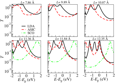
Fig.  11: Transmission coefficients as a function of energy for different electrode separation for the Au-BDT-Au junctions. Comparison between LDA, ASIC and LDA+SCO.

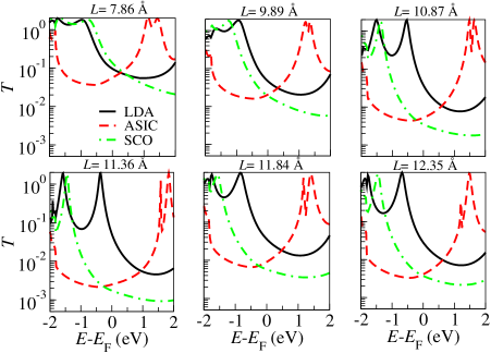
Fig.  12: Transmission coefficients as a function of energy for different electrode separation for the Au-BDT2H-Au junctions. Comparison between LDA, ASIC and LDA+SCO.

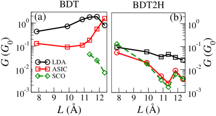
Fig.  13: Conductance as a function of $L$ for (a) Au-BDT-Au and (b) Au-BDT2H-Au molecular junctions. Comparison between LDA, ASIC and scissor operator (SCO) results.

Recently, using low-temperature MCBJs Bruot et al. ²² observed some conductance traces where $G$ changed from 0.01$G_{0}$ to 0.1$G_{0}$ by increasing $L$. The authors attributed this to the HOMO level moving up in energy towards the $E_{\mathrm{F}}$ of the electrodes. However, most experimental results ^{8, 17, 9, 6, 18, 4, 3, 2, 19, 20, 21, 7, 23, 24, 25, 26, 27, 28, 5, 29} show conductance traces with either approximately constant $G$ under stretching, or with decreasing $G$ for increasing $L$.^{84, 9} In the calculations of French et al. ¹⁶ two types of conductance traces are found: (i) large increase under stretching and (ii) approximately constant values. The increase of $G$ is found only for junctions that form monoatomic chains (MACs) of gold atoms connected to the BDT molecules. MAC formation leads to an increase of the DOS at $E_{\mathrm{F}}$ in the contact Au atoms, which adds to the increase of $G$ due to the HOMO shifting closer to $E_{\mathrm{F}}$ under stretching.

By applying the ASIC the absolute value of $G$ decreases by up to one order of magnitude when compared to the LDA values, since the HOMO level is shifted to lower energies (Fig. 11). For small $L$ the ASIC $G$ vs. $L$ curve is approximately constant, while for large $L$ the value of $G$ is found to increase for large $L$ [Fig. 13(a)], which is also due to the fact that the HOMO level ($\Psi_{1}$) is approaching $E_{\mathrm{F}}$ as the junction is stretched. Our CDFT results of the previous section show that for $L\geq 11.36$ Å the $\Psi_{1}$ state is expected to be located at least $\sim$1.5 eV above $E_{\mathrm{F}}$. Thus we apply the SCO to shift the eigenvalue of $\Psi_{1}$ to this energy, and calculate the transmission (green-dashed lines) and $G$ (for $L\geq 11.36$ Å ) by using the calculated corrections presented in Table. 3. The corrected $G$ is smaller than the LDA results by up to two orders of magnitude and smaller than the ASIC by about a factor of 10.

In contrast, for the Au-BDT2H-Au structures, $G$ decreases with increasing $L$ for all used XC functionals (Fig. 12). For LDA $G$ monotonically decreases from 0.1$G_{0}$ to 0.026$G_{0}$, and using ASIC the values of $G$ further decrease by up to one order of magnitude. Applying the SCO correction $E_{\mathrm{LDA}}^{\mathrm{gap}}$ increases, and consequently $G$ decreases by more than one order of magnitude when compared to the LDA results, except for the shortest considered distance. We note that although $G$ is similar for ASIC and SCO, $T$ at $E_{\mathrm{F}}$ is dominated by the LUMO tail for ASIC (see Fig. 12), while it is HOMO dominated for SCO. The agreement between ASIC and SCO is mainly due to the fact that both put $E_{\mathrm{F}}$ in the gap, and the change of $G$ with stretching is mainly due to the change of the electronic coupling to the electrodes. The decreasing trend of $G$ vs. $L$ was observed by Ning et al. ³⁸ where they considered the Au-BDT2H-Au junctions and the molecule is symmetrically connected to an adatom structure. This is qualitatively in good agreement with the experiments of Kim et al. ⁹, where by means of low-temperature MCBJ technique, they reported values of $G$ ranging from $6.6\times 10^{-4}$ to 0.5$G_{0}$ and that high-conductance values are obtained when the molecular junction is compressed, i.e, $L$ decreases. These are the key results of the present work since when combined with the results for the formation energy of the hydrogenated junctions, they indicate that the possibility of having thiol junctions can not be ruled out. In fact, the thiol structures might be the ones present in junctions where $G$ decreases with elongation.^{84, 9}

An important difference between the Au-BDT-Au and Au-BDT2H-Au junctions is the character of the charge carriers, i.e., whether it is hole-like or electron-like transport. For Au-BDT-Au, in the strong coupling limit where $L\leq 10.87$ Å, the charges tunnel through the tail of the HOMO-like level which leads to a hole-like transport (see top panel of Fig. 11). In the weak coupling limit, after considering the SCO, the charge carriers tunnel through the tail of the LUMO-like level which leads to a electron-like transport, as shown in the bottom panel of Fig. 11. For Au-BDT2H-Au junctions, the tunneling is always performed through the tail of the HOMO-like level (see Fig. 12) and therefore the charge carriers are holes. This is an important information since, experimentally, by means of thermoelectric transport measurements, it is possible to address which frontier molecular level is the conducting level. It has been shown ²⁵ that for the systems discussed, this level is the HOMO, which agrees with our findings for the Au-BDT2H-Au junctions and also for the Au-BDT-Au junctions in the strong coupling limit. This leads to the conclusion that for experiments where $G$ increases with stretching, ²² the thiolate junction is present and the explanation for this observed trend can be due to the formation of the MACs proposed by French et al..¹⁶ In contrast, the thiol structures might be the ones present in experimental measurements showing the opposite trend.^{84, 9}

4 Conclusion

We performed DFT calculations to study the adsorption process of methanethiol and BDT2H molecules on the Au(111) surface. For all the structures studied we find that thiols are energetically more stable than their thiolate counterparts. Moreover, we find a large activation barrier of about 1 eV for the the dissociation of the H atom from the thiol groups adsorbed on Au(111). These results indicate that the non-dissociated structures are likely to exist in experiments, and therefore can not be ruled out.

The energy level alignment between molecule and electrodes is one of the main factors that determine the conductance. To overcome the limitations of using the LDA-DFT eigenvalues we apply a CDFT method, which is based on total energy differences in the same way as $\Delta$SCF calculations, with the difference that it allows also the inclusion of the non-local Coulomb interaction that leads to the renormalization of energy levels as the molecule is brought close to a metal surface. We find a reduction of the BDT $E_{\mathrm{QP}}^{\mathrm{gap}}$ of 2.09 eV with respect to its gas phase gap, when the molecule is brought closer to a single Au(111) surface. CDFT also allows us to obtain the height of the image charge plane on Au(111), which we find to be at about 1 Å  above the gold surface. While for the BDT2H molecules the coupling to the surface remains small at all distances, for small molecule-surface separation the electronic coupling between BDT and Au becomes very strong, and in this limit the use of the CDFT approach is not applicable. The strong coupling leads to a significant electron transfer from the surface to the molecule, so that the molecular LUMO of isolated BDT becomes increasingly occupied as the molecule-surface distance decreases. When we correct for the self-interaction error in the LDA XC functional, the electron transfer is enhanced. At the equilibrium Au(111)-BDT bonding distance we then find that the molecular LUMO of isolated BDT has become fully filled. On the other hand, for BDT2H, the filling of the molecular orbitals does not depend on the distance to Au.

By means of NEGF+DFT we have then calculated the transport properties of the junctions with different contact geometries and compare the results obtained with LDA, ASIC and LDA+SCO functionals. For the thiol structures, the LDA values for $G$ are about one order of magnitude smaller than their thiolate counterparts. ASIC leads to values of $G$ in better agreement with experiments for the thiolate systems. However, ASIC also leads to a spurious increase of $G$ for the thiol junctions due to the down-shift of the empty states towards $E_{\mathrm{F}}$, an artifact avoided in the SCO approach. We find that Au-BDT-Au and Au-BDT2H-Au junctions show opposite trends concerning the dependence of $G$ on the separation between flat Au electrodes; $G$ decreases with $L$ for the thiol junctions, whereas the thiolates show the opposite trend. Since for Au-BDT2H-Au there is no significant charge transfer between the electrodes and the molecule, we can apply the SCO approach to set the HOMO-LUMO gap to the one obtained from CDFT calculations. In this way $G$ decreases by up to two orders of magnitude when compared to the LDA values, and this brings the results in good quantitative agreement with the experimental data. Our results therefore suggest that thiol junctions must be present in experiments where $G$ decreases with $L$. In contrast, thiolates structures are likely to be present in experiments showing a increase of the conductance upon stretching.

References

- Reed 1997 M. A. Reed, C. Zhou, C. J. Muller, T. P. Burgin, and J. M. Tour, Science, 1997, 278, 252–254.
- Tsutsui et al. 2006 M. Tsutsui, Y. Teramae, S. Kurokawa and A. Sakai, Appl. Phys. Lett., 2006, 89, 163111–163113.
- Tsutsui et al. 2009 M. Tsutsui, M. Taniguchi, K. Shoji, K. Yokota and T. Kawai, Nanoscale, 2009, 1, 164–170.
- Tian et al. 2010 J.-H. Tian, Y. Yang, X.-S. Zhou, B. Schöllhorn, E. Maisonhaute, Z.-B. Chen, F.-Z. Yang, Y. Chen, C. Amatore, B.-W. Mao and Z.-Q. Tian, ChemPhysChem., 2010, 11, 2745–2755.
- Xu et al. 2004 X. Xiao, B. Xu, and N. J. Tao, Nano Lett., 2004, 4, 267–271.
- Taniguchi et al. 2010 M. Taniguchi, M. Tsutsui, K. Yokota and T. Kawai, Chem. Sci., 2010, 1, 247–253.
- Baheti et al. 2008 K. Baheti, J. A. Malen, P. Doak, P. Reddy, S.-Y. Jang, T. D. Tilley, A. Majumdar and R. A. Segalman, Nano Lett., 2008, 8, 715–719.
- Lörtscher et al. 2007 E. Lörtscher, H. B Weber and H. Riel, Phys. Rev. Lett., 2007, 98, 176807–176811.
- Kim et al. 2011 Y. Kim, T. Pietsch, A. Erbe, W. Belzig and E. Scheer, Nano Lett., 2011, 11, 3734–3738.
- Demir and Kirczenow 2012 F. Demir and G. Kirczenow, J. Chem. Phys., 2012, 137, 094703–094713.
- Pontes et al. 2006 R. B. Pontes, F. D. Novaes, A. Fazzio and A. J. R. Silva, J. Am. Chem. Soc., 2006, 128, 8996–8997.
- Pontes et al. 2011 R. B. Pontes, A. R. Rocha, S. Sanvito, A. Fazzio and A. J. R. Da Silva, ACS Nano, 2011, 5, 795–804.
- Toher and Sanvito 2008 C. Toher and S. Sanvito, Phys. Rev. B, 2008, 77, 155402–155414.
- Strange and Thygesen 2011 M. Strange and K. S. Thygesen, arXiv:cond-mat/1108-3687v1, 2011.
- French et al. 2013 W. R. French, C. R. Iacovella, I. Rungger, A. M. Souza, S. Sanvito and P. T. Cummings, J. Phys. Chem. Lett., 2013, 4, 887–891.
- French et al. 2013 W. R. French, C. R. Iacovella, I. Rungger, A. M. Souza, S. Sanvito and P. T. Cummings, Nanoscale, 2013, 5, 3654–3663.
- Gonzalez et al. 2006 M. T. Gonzalez, S. Wu, R. Huber, S. J. van der Molen, C. Schönenberger and M. Calame, Nano Lett., 2006, 6, 2238–2242.
- Tian et al. 2006 J.-H. Tian, B. Liu, X. Li, Z.-L. Yang, B. Ren, S.-T. Wu, N. Tao and Z.-Q. Tian, J. Am. Chem. Soc., 2006, 128, 14748–14749.
- Tsutsui et al. 2009 M. Tsutsui, M. Taniguchi and T. Kawai, Nano Lett., 2009, 9, 2433–2439.
- Quek et al. 2009 S. Y. Quek, M. Kamenetska, M. L. Steigerwald, H. J. Choi, S. G. Louie, M. S. Hybertsen, J. B. Neaton and L. Venkataraman, Nat. Nanotech. 2009, 4, 230–234.
- Arroyo et al. 2011 C. R. Arroyo, E. Leary, A. Castellanos-Gómez, G. Rubio-Bollinger, M. T. González and N. Agraït, J. Am. Chem. Soc., 2011, 133, 14313–14319.
- Bruot et al. 2012 C. Bruot, J. Hihath and N. Tao, Nat. Nanotech., 2012, 7, 35–40.
- Fatemi et al. 2011 V. Fatemi, M. Kamenetska, J. B. Neaton and L. Venkataraman, Nano Lett., 2011, 11, 1988–1992.
- Kiguchi et al. 2010 M. Kiguchi, H. Nakamura, Y. Takahashi, T. Takahashi and T. Ohto, J. Phys. Chem. C, 2010, 114, 22254–22261.
- Reddy et al. 2007 P. Reddy, S.-Y. Jang, R. A. Segalman and A. Majumdar, Science (New York, N.Y.), 2007, 315, 1568–1571.
- Vazquez et al. 2012 H. Vazquez, R. Skouta, S. Schneebeli, M. Kamenetska, R. Breslow, L. Venkataraman and M. S. Hybertsen, Nat. Nanotech., 2012, 7, 663–667.
- Venkataraman et al. 2006 L. Venkataraman, J. E. Klare, I. W. Tam, C. Nuckolls, M. S. Hybertsen and M. L. Steigerwald, Nano Lett., 2006, 6, 458–462.
- Wold et al. 2002 D. J. Wold, R. Haag, M. A. Rampi and C. D. Frisbie, J. Phys. Chem. B, 2002, 106, 2813–2816.
- Xu and Tao 2003 B. Xu and N. J. Tao, Science (New York, N.Y.), 2003, 301, 1221–1223.
- Tomfohr and Sankey 2004 J. Tomfohr and O. F. Sankey, J. Chem. Phys., 2004, 120, 1542–1554.
- Stokbro et al. 2003 K. Stokbro, J. Taylor, M. Brandbyge, J.-L. Mozos and P. Ordejón, Comp. Mat. Sci., 2003, 27, 151–160.
- Maksymovych and Yates 2008 P. Maksymovych and J. T. Yates, J. Am. Chem. Soc., 2008, 130, 7518–7519.
- Andreoni et al. 2000 W. Andreoni, A. Curioni and H. Grönbeck, Int. J. Q. Chem., 2000, 80, 598–608.
- Pu et al. 2010 Q. Pu, Y. Leng, X. Zhao and P. T. Cummings, J. Phys. Chem. C, 2010, 114, 10365–10372.
- Strange et al. 2011 M. Strange, C. Rostgaard, H. Häkkinen and K. S. Thygesen, Phys. Rev. B, 2011, 83, 115108–115120.
- Grönbeck et al. 2000 H. Grönbeck, A. Curioni and W. Andreoni, J. Am. Chem. Soc., 2000, 122, 3839–3842.
- Nara et al. 2004 J. Nara, S. Higai, Y. Morikawa and T. Ohno, J. Chem. Phys., 2004, 120, 6705–6711.
- Ning et al. 2010 Z. Ning, W. Ji and H. Guo, arXiv:cond-mat/09074674v2, 2010.
- Perdew and Levy 1983 J. P. Perdew and M. Levy, Phys. Rev. Lett., 1983, 51, 1884–1887.
- Perdew et al. 1982 J. P. Perdew, R. G. Parr, M. Levy and J. L. Balduz, Phys. Rev. Lett., 1982, 49, 1691–1694.
- J. F. Janak 1978 J. F. Janak, Phys. Rev. B, 1978, 18, 7165–7168.
- Hesper et al. 1997 R. Hesper, L. H. Tjeng and G. A. Sawatzky, Europhys. Lett., 1997, 40, 177–182.
- Repp et al. 2005 J. Repp, G. Meyer, S. Stojković, A. Gourdon and C. Joachim, Phys. Rev. Lett., 2005, 94, 026803–026807.
- Lu et al. 2004 X. Lu, M. Grobis, K. H. Khoo, S. G. Louie and M. F. Crommie, Phys. Rev. B, 2004, 70, 115418–115426.
- Greiner et al. 2011 M. T. Greiner, M. G. Helander, W.-M. Tang, Z.-B. Wang, J. Qiu and Z.-H. Lu, Nat. Mat., 2011, 11, 76–81.
- Perrin et al. 2013 M. L. Perrin, C. J. O. Verzijl, C. A. Martin, A. J. Shaikh, R. Eelkema, J. H. van Esch, J. M. van Ruitenbeek, J. M. Thijssen, H. S. J. van der Zant and D. Dulić, Nat. Nanotech., 2013, 8, 282–287.
- kronik 2008 S. Kümmel and L. Kronik, Rev. Mod. Phys., 2008, 80, 3–60.
- Flores 2009 F. Flores, J. Ortega and H. Vázquez, Phys. Chem. Chem. Phys., 2009, 11, 8658–8675.
- Inkson 1973 J. C. Inkson, J. Phys. C: Solid State Phys., 1973, 6, 1350–1362.
- Hybertsen and Louie 1986 M. S. Hybertsen and S. G. Louie, Phys. Rev. B, 1986, 34, 5390–5413.
- Onida et al. 2002 G. Onida, L. Reining and A. Rubio, Rev. Mod. Phys., 2002, 74, 601–659.
- Neaton et al. 2006 J. B. Neaton, M. S. Hybertsen and S. G. Louie, Phys. Rev. Lett., 2006, 97, 216405–216409.
- Garcia-Lastra and Thygesen 2011 J. M. Garcia-Lastra and K. S. Thygesen, Phys. Rev. Lett., 2011, 106, 187402–187406.
- Garcia-Lastra et al. 2009 J. M. Garcia-Lastra, C. Rostgaard, A. Rubio and K. S. Thygesen, Phys. Rev. B, 2009, 80, 245427–245434.
- Tamblyn et al. 2011 I. Tamblyn, P. Darancet, S. Y. Quek, S. A. Bonev and J. B. Neaton, Phys. Rev. B, 2011, 84, 201402–201406.
- Rignanese et al. 2001 G.-M. Rignanese, X. Blase and S. G. Louie, Phys. Rev. Lett., 2001, 86, 2110–2113.
- Strange and Thygesen 2012 M. Strange and K. S. Thygesen, Phys. Rev. B, 2012, 86, 195121–195127.
- Pemmaraju et al. 2007 C. D. Pemmaraju, T. Archer, D. Sánchez-Portal and S. Sanvito, Phys. Rev. B, 2007, 75, 045101–045116.
- Quek et al. 2007 S. Y. Quek, L. Venkataraman, H. J. Choi, S. G. Louie, M. S. Hybertsen and J. B. Neaton, Nano Lett., 2007, 7, 3477–3482.
- García-Suárez and Lambert 2011 V. M. García-Suárez and C. J. Lambert, New J. Phys., 2011, 13, 053026–05342.
- Souza et al. 2013 A. M. Souza, I. Rungger, C. D. Pemmaraju, U. Schwingenschloegl and S. Sanvito, Phys. Rev. B, 2013, 88, 165112–165121.
- Soler et al. 2002 J. M. Soler, E. Artacho, J. D. Gale, A. García, J. Junquera, P. Ordejón and D. Sánchez-Portal, J. Phys.: Condens. Matter, 2002, 14, 2745–2779.
- Kresse and Furthmer 1996 G. Kresse and J. Furthmüller, Phys. Rev. B, 1996, 54, 11169–11186.
- Perdew et al. 1996 J. P. Perdew, K. Burke and M. Ernzerhof, Phys. Rev. Lett., 1996, 77, 3865–3868.
- Troullier and Martins 1991 N. Troullier and J. L. Martins, Phys. Rev. B, 1991, 15, 43–57.
- Rostgaard 2009 C. Rostgaard, arXiv:cond-mat/09101921v2, 2009.
- Rungger 2008 I. Rungger and S. Sanvito, Phys. Rev. B, 2008, 78, 035407–035420.
- Rocha et al. 2006 A. R. Rocha, V. M. García-Suárez, S. Bailey, C. J. Lambert, J. Ferrer and S. Sanvito, Phys. Rev. B, 2006, 73, 085414–085435.
- Filippetti et al. 2011 A. Filippetti, C. D. Pemmaraju, S. Sanvito, P. Delugas, D. Puggioni and V. Fiorentini, Phys. Rev. B, 2011, 84, 195127–195149.
- Toher et al. 2005 C. Toher, A. Filippetti, S. Sanvito and K. Burke, Phys. Rev. Lett., 2005, 95, 146402–146406.
- Lang and Kohn 1973 N. D. Lang and W. Kohn, Phys. Rev. B, 1973, 7, 3541–3551.
- Ferretti et al. 2005 A. Ferretti, A. Calzolari, R. Di Felice and F. Manghi, Phys. Rev. B, 2005, 72, 125114–125127.
- Quek et al. 2011 S. Y. Quek, H. J. Choi, S. G. Louie and J. B. Neaton, ACS Nano, 2011, 5, 551–557.
- Mowbray et al. 2008 D. J. Mowbray, G. Jones and K. S. Thygesen, J. Chem. Phys., 2008, 128, 111103–111108.
- Abad et al. 2008 E. Abad, J. Ortega, Y. J. Dappe and F. Flores, Appl. Phys. A, 2008, 95, 119–124.
- Zhou and Hagelberg 2006 J.-G. Zhou and F. Hagelberg, Phys. Rev. Lett., 2006, 97, 045505–045509.
- Lee et al. 2005 I. I. Rzeźnicka, J. Lee, P. Maksymovych and J. T. Yates, J. Phys. Chem. B, 2005, 109, 15992–15996.
- Nuzzo et al. 1987 R. G. Nuzzo, B. R. Zegarski and L. H. Dubois, J. Am. Chem. Soc., 1987, 109, 733–740.
- Henkelman 2000 G. Henkelman, B. P. Uberuaga and H. Jónsson, J. Chem. Phys., 2000, 113, 9901–9904.
- Henkelman2 2000 G. Henkelman and H. Jónsson, J. Chem. Phys., 2000, 113, 9978–9985.
- Henkelman3 2000 G. Henkelman and H. Jónsson, J. Chem. Phys., 2000, 111, 7010–7022.
- Frei et al. 2012 M. Frei, S. V. Aradhya, M. S. Hybertsen and L. Venkataraman, J. Am. Chem. Soc., 2012, 134, 4003–4006.
- Aradhya et al. 2012 S. V. Aradhya, M. Frei, M. S. Hybertsen and L. Venkataraman, Nat. Mat., 2012, 11, 872–878.
- Huang et al. 2006 Z. Huang, B. Xu, Y. Chen, M. Di Ventra and N. Tao, Nano Lett., 2006, 6, 1240–1244.
- Li et al. 2006 X. Li, J. He, J. Hihath, B. Xu, S. M. Lindsay and N. Tao, J. Am. Chem. Soc., 2006, 128, 2135–2141.
- Strange et al. 2010 M. Strange, O. Lopez-Acevedo and H. Häkkinen, J. Phys. Chem. Lett., 2010, 1, 1528–1532.
- Romaner et al. 2006 L. Romaner, G. Heimel, M. Gruber, J.-L. Brédas and E. Zojer, Small, 2006, 2, 1468–1475.
- Sergueev et al. 2010 N. Sergueev, L. Tsetseris, K. Varga and S. Pantelides, Phys. Rev. B, 2010, 82, 073106–073110.
- Qi et al. 2009 Y. Qi, J. Qin, G. Zhang and T. Zhang, J. Am. Chem. Soc., 2009, 131, 16418–16422.