A new ray-tracing scheme for 3D diffuse radiation transfer on highly parallel architectures

Abstract

We present a new numerical scheme to solve the transfer of diffuse radiation on three-dimensional mesh grids which is efficient on processors with highly parallel architecture such as recently popular GPUs and CPUs with multi- and many-core architectures. The scheme is based on the ray-tracing method and the computational cost is proportional to $N_{\rm m}^{5/3}$ where $N_{\rm m}$ is the number of mesh grids, and is devised to compute the radiation transfer along each light-ray completely in parallel with appropriate grouping of the light-rays. We find that the performance of our scheme scales well with the number of adopted CPU cores and GPUs, and also that our scheme is nicely parallelized on a multi-node system by adopting the multiple wave front scheme, and the performance scales well with the amount of the computational resources. As numerical tests to validate our scheme and to give a physical criterion for the angular resolution of our ray-tracing scheme, we perform several numerical simulations of the photo-ionization of neutral hydrogen gas by ionizing radiation sources without the “on-the-spot” approximation, in which the transfer of diffuse radiation by radiative recombination is incorporated in a self-consistent manner.

1 Introduction

Radiation transfer (RT) has been long recognized as a indispensable ingredient in numerically simulating many astrophysical phenomena including the reionization of intergalactic medium (IGM) in the early universe, radiative feedback during the galaxy formation, and others. So far, varieties of numerical schemes for solving the RT in three dimensions are proposed during the last two decades (Iliev et al., 2006), and some of them can be coupled with the hydrodynamic simulations (Iliev et al., 2009) thanks to not only the increase of the available computational resources, but also the improvement of numerical algorithms to solve the RT in many astrophysical conditions.

Most of the numerical schemes for RT can be divided into two groups: one is the moment-based schemes which solve the moment equation of the RT equation instead of solving the RT equation directly, and the other is the ray-tracing schemes. As for the moment-based schemes, the important advantage is that the computational costs scale with the number of mesh grids, $N_{\rm m}$ and hence can be easily coupled with hydrodynamic simulations. The flux-limited diffusion (FLD) scheme, which adopts the closure relation valid in the diffusion limit, is the most common among the moment-based schemes, while there are a number of more sophisticated schemes which close the moment equations with the optically thin variable Eddington tensor approximation (Gnedin & Abel, 2001) and the locally evaluated Eddington tensor (the M₁ model) (González, Audit & Huynh, 2007; Skinner & Ostriker, 2013; Kanno et al., 2013). The accuracy and validity of the moment-based schemes are, however, problem-dependent. For example, the FLD scheme has a problem in handling shadows formed behind opaque objects (González, Audit & Huynh, 2007). While schemes with M₁ model are capable of simulating shadows sucessfully, they cannot solve the crossing of multiple beamed lights, where the beamed lights unphysically merge into one beam (Rosdahl et al., 2013). Therefore, the ray-tracing schemes are naturally chosen for solving the RT in situations that we are considering in the studies of galaxy formation and cosmic reionization, in which there exist a number of radiation sources.

In ray-tracing schemes, emission and absorption of radiation are followed along the light-rays that extend through the computational domain. As for the long-characteristics schemes (Abel, Norman & Madau, 1999; Sokasian et al., 2001) in which light-rays between all radiation sources and all other relevant meshes are considered, the computational cost scales with $N_{\rm m}^{2}$ in general cases and $N_{\rm m}^{4/3}N_{\rm s}$ when we consider only the RT from point radiating sources, where $N_{\rm s}$ is the number of point sources. On the other hand, for the short-characteristics schemes (Kunasz & Auer, 1988; Stone et al., 1992) which are similar to the long-characteristics schemes but integrate the RT equation only along paths connecting nearby mesh grids, the computational cost scales with $N_{\rm m}^{5/3}$ in general and $N_{\rm m}N_{\rm s}$ for the RT from point sources. Ray-tracing schemes are in principle versatile for any physical settings but computationally much more expensive than the moment-based schemes. Due to such huge computational costs, RT simulations with the ray-tracing schemes have been applied only to static conditions or snapshots of hydrodynamical simulations in a post-process manner in many previous studies.

Some of the ray-tracing schemes are now coupled with hydrodynamical simulations adopting smoothed particle hydrodynamics (SPH) codes (Susa, 2006; Hasegawa & Umemura, 2010; Pawlik & Schaye, 2011) and mesh-based codes (Rijkhorst et al., 2006; Wise & Abel, 2011), and they can handle the RT and its hydrodynamical feedback in a self-consistent manner. Majority of these radiation hydrodynamics codes, however, consider the transfer of radiation only from point sources and ignore the effect of radiation transfer from spatially extended diffuse sources, such as the recombination radiation emitted from ionized regions and infrared radiation emitted by dust grains, since the computational costs for computing the transfer of diffuse radiation is prohibitively large.

Specifically, in the numerical RT calculations of the hydrogen ionizing radiation, we usually adopt the on-the-spot approximation in which one assumes that the ionizing photons emitted by radiative recombinations in ionized regions are absorbed by neutral atoms in the immediate vicinity of the recombining atoms. However, adopting the on-the-spot approximation can fail to notice the important effects of diffuse recombination radiation in some situations. The roles of ionizing recombination photons in the epoch of cosmic reionization is discussed by a number of works (Ciardi et al., 2001; Miralda-Escudé, 2003; Dopita et al., 2011; Rahmati et al., 2013a). Dopita et al. (2011) proposed the recombination photons produced in the fast accretion shocks in the structure formation in the universe as an possible source of ionizing photons responsible for the cosmic reionization, though Wyithe et al. (2011) showed that its impact on the cosmic reionization is not very significant. It is also reported that the recombination radiation plays an important role at transition regions between highly ionized and self-shielded regions (Rahmati et al., 2013a). As for the effect of recombination photons on the galaxy-size scales, Inoue (2010) showed that the recombination radiation produces the Lyman-‘bump’ feature in the spectral energy distributions of high-$z$ galaxies, and also that the escaping ionizing photons from high-$z$ galaxies are to some extent contributed by the recombination radiation. Rahmati et al. (2013b) also pointed out that the recombination radiation makes the major contribution to the photo-ionization at regions where the gas is self-shielded from the UV background radiation.

The RT of infrared diffuse radiation emitted by dust grains plays an important roles in the evolution of star-forming galaxies, in which the radiation pressure exerted by multi-scattered infrared photons drives stellar winds. In most of numerical simulations of galaxy formation, however, such momentum transfer is treated only in a phenomenological manner (e.g. Okamoto et al. 2014).

In this paper, we present a new ray-tracing scheme to solve the RT of diffuse radiation from spatially extended radiating sources efficiently on processors with highly parallel architectures such as graphics processing units (GPUs) and multi-core CPUs which are recently popular or available in near future. The basic idea of the scheme is based on the scheme presented by Razoumov & Cardall (2005) and ‘Authentic Radiation Transfer’ (ART) scheme Nakamoto et al. (2001b). Generally speaking, development of such numerical schemes with high concurrency is of critical importance because the performance improvement of recent processors are achieved by the increase of the number of processing elements or CPU cores integrated on a single processor chip rather than the improvement of the performance of individual processing elements.

The rest of the paper is organized as follows. Section 2 is devoted to describe the numerical scheme to simulate the radiation transfer. In section 3, we present our implementation of the scheme suitable to highly parallel architectures such as GPUs and CPUs with multi-core architectures. We present the results of numerical test suits of RT of diffuse radiation in Section 4. The computational performance of our implementation is shown in Section 5. Finally, we summarize our results in Section 6.

2 Methodology

In this section, we describe our ray-tracing scheme of diffuse radiation transfer. Generally, the radiation field can be decomposed into two components. One is the direct incident radiation from point radiation sources, and the other is the diffuse radiation emerged from spatially extended regions. In our implementation, the RT of photons emitted by point radiation sources is computed separately from that of diffuse radiation. Throughout in this paper, we consider the RT of hydrogen ionizing photons emitted by point radiation sources, and recombination photons emerged from the ionized regions as the diffuse radiation. We use the steady state RT equation for a given frequency $\nu$:

$$\frac{dI_{\nu}}{d\tau_{\nu}}=-I_{\nu}+\mathcal{S}_{\nu},$$ (1)

where $I_{\nu},\tau_{\nu}$ and $\mathcal{S}_{\nu}$ are the specific intensity, the optical depth and the source function, respectively. The source function is given by $\mathcal{S}_{\nu}=\varepsilon_{\nu}/\kappa_{\nu},$ where $\kappa_{\nu}$ and $\varepsilon_{\nu}$ are the absorption and emission coefficients, respectively. The formal solution of this equation is given by

$$I_{\nu}(\tau_{\nu})=I_{\nu}(0)\,e^{-\tau_{\nu}}+\int^{\tau_{\nu}}_{0}\mathcal{S}_{\nu}(\tau^{\prime}_{\nu})e^{-(\tau_{\nu}-\tau^{\prime}_{\nu})}d\tau^{\prime}_{\nu},$$ (2)

where $\tau^{\prime}_{\nu}$ is the optical depth at a position along the ray. When we adopt the “on-the-spot” approximation in which recombination photons emitted in ionized regions are assumed to be absorbed where they are emitted, we neglect the source function, $\mathcal{S}_{\nu}$, and the formal solution is simply reduced to

$$I_{\nu}(\tau_{\nu})=I_{\nu}(0)\,e^{-\tau_{\nu}}.$$ (3)

2.1 RT from point radiation sources

To solve the RT from point radiation sources, we compute the optical depth between each pair of a point radiation source and a target mesh grid, i.e. an end point of each light-ray (see Figure 1). Instead of solving equation (3), we compute the radiation flux density at the target mesh grid as

$$f_{\alpha}(\nu)=\frac{L_{\alpha}(\nu)}{4\pi r_{\alpha}^{2}}\,\exp\left[-\tau_{\alpha}(\nu)\right],$$ (4)

where $L_{\alpha}(\nu)$ is the intrinsic luminosity of the $\alpha$-th point radiation source, and $r_{\alpha}$ and $\tau_{\alpha}(\nu)$ are the distance and the optical depth between the point radiation source and the target mesh grid, respectively. Then, the photo-ionization and photo-heating rates of the $i$-th species contributed by the $\alpha$-th point radiation source are computed by

$$\Gamma^{\alpha}_{i,\gamma}=\int^{\infty}_{\nu_{i}}\frac{f_{\alpha}(\nu)}{h\nu}\sigma_{i}(\nu)\,d\nu,$$ (5)

and

$$\mathcal{H}^{\alpha}_{i,\gamma}=\int^{\infty}_{\nu_{i}}\frac{f_{\alpha}(\nu)}{h\nu}(h\nu-h\nu_{i})\sigma_{i}(\nu)\,d\nu$$ (6)

respectively, where $\sigma_{i}(\nu)$ and $\nu_{i}$ are the ionization cross section and the threshold frequency of the $i$-th species, respectively. In the test simulations desribed in this paper, we compute these photo-ionization and photo-heating rates in a photon-conserving manner (Abel, Norman & Madau, 1999) as described in appendix  A.

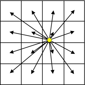
Figure 1: Schematic illustration of the ray-tracing method for the radiation emitted by a point radiation source in the two-dimensional mesh grids.

For a single point radiation source, the number of rays to be calculated is $N_{\rm m}$, and the number of mesh grids traveled by a single light-ray is in the order of $N^{1/3}_{\rm m}$. Thus, the computational cost for a single point radiation source is proportional to $N^{4/3}_{\rm m}$. Therefore, the total computational cost scales as $N_{\rm m}^{4/3}N_{\rm s}$, where $N_{\rm s}$ is the number of point radiation sources. For a large number of point radiation sources, we can mitigate the computational costs by adopting more sophisticated scheme such as the ARGOT scheme (Okamoto et al., 2012) in which a distant group of point radiation sources is treated as a bright point source located at the luminosity center with a luminosity summed up for all the sources in the group to effectively reduce the number of radiation sources and hence the computational cost is proportional to $N^{4/3}_{\rm m}\log N_{\rm s}$.

2.2 RT of the diffuse radiation

We solve the equation (2) to compute the RT of the diffuse radiation. The numerical scheme we adopt in this work is based on the method developed by Razoumov & Cardall (2005) and ART scheme (Nakamoto et al., 2001b; Iliev et al., 2006), which is reported to have little numerical diffusion in the searchlight beam test like the long characteristics method although its computational cost is proportional to $N_{\rm m}^{5/3}$ similarly to that of the short characteristic method (Nakamoto et al., 2001b). In this scheme, we solve the equation (2) along equally spaced parallel rays as schematically shown in Figure 2.

For a given incoming radiation intensity $I^{\rm in}_{\nu}$ along a direction $\hat{\mathbf{n}}$, the outgoing radiation intensity $I^{\rm out}_{\nu}$ after getting through a path length $\Delta L$ of a single mesh is computed by integrating equation (2) as

$$I^{\rm out}_{\nu}(\hat{\mathbf{n}})=I^{\rm in}_{\nu}(\hat{\mathbf{n}})\,e^{-\Delta\tau_{\nu}}+\mathcal{S}_{\nu}(1-e^{-\Delta\tau_{\nu}}),$$ (7)

where $\Delta\tau_{\nu}$ is the optical depth of the path length $\Delta L$ (i.e. $\Delta\tau_{\nu}=\kappa_{\nu}\Delta L$), and $\mathcal{S}_{\nu}$ and $\kappa_{\nu}$ are the source function and the absorption coefficient of the mesh grid, respectively.

The intensity of the incoming radiation averaged over the path length $\Delta L$ across a single mesh grid can be calculated as

$$\bar{I}^{\rm in}_{\nu}(\hat{\mathbf{n}})=\frac{1}{\Delta L}\int_{0}^{\Delta L}I^{\rm in}_{\nu}(\hat{\mathbf{n}})e^{-\kappa_{\nu}l}\,dl=I_{\nu}^{\rm in}(\hat{\mathbf{n}})\frac{1-e^{-\Delta\tau_{\nu}}}{\Delta\tau_{\nu}}.$$ (8)

In addition to this, we have a contribution to the radiation intensity from the source function which we set constant in each mesh grid, and the total intensity averaged over the path length is given by

$$\bar{I}_{\nu}(\hat{\mathbf{n}})=\bar{I}^{\rm in}_{\nu}(\hat{\mathbf{n}})+\mathcal{S}_{\nu}=I_{\nu}^{\rm in}(\hat{\mathbf{n}}_{i})\frac{1-e^{-\Delta\tau_{\nu}}}{\Delta\tau_{\nu}}+\mathcal{S}_{\nu}$$ (9)

For those mesh grids through which multiple parallel light-rays pass, the averaged intensity can be given by

$$\bar{I}_{\nu}^{\rm ave}(\hat{\mathbf{n}})=\frac{\sum_{j}\Delta\tau_{\nu,j}\bar{I}_{\nu,j}(\hat{\mathbf{n}})}{\sum_{j}\Delta\tau_{\nu,j}}=\bar{I}_{\nu}^{\rm ave,in}(\hat{\mathbf{n}})+\mathcal{S}_{\nu},$$ (10)

where $\bar{I}_{\nu,i}$ and $\Delta\tau_{\nu,i}$ are the intensity averaged over the $i$-th light-ray and the optical depth of $i$-th light-ray in the mesh grids, respectively, $\bar{I}^{\rm ave,in}_{\nu}$ is a contribution from the incoming radiation given by

$$\bar{I}^{\rm ave,in}_{\nu}(\hat{\mathbf{n}})=\frac{\sum_{j}\Delta\tau_{\nu,j}\bar{I}^{\rm in}_{\nu,j}(\hat{\mathbf{n}})}{\sum_{j}\Delta\tau_{\nu,j}},$$ (11)

and the summation is over all the parallel light-rays in the same mesh grid. Then, the mean intensity can be computed by averaging $\bar{I}^{\rm ave}_{\nu}$ described above over all the directions as,

$$J_{\nu}=\frac{1}{N_{\rm d}}\sum_{i=1}^{N_{\rm d}}\bar{I}_{\nu}^{\rm ave}(\hat{\mathbf{n}}_{i})=J^{\rm in}_{\nu}+\mathcal{S}_{\nu},$$ (12)

where $\hat{\mathbf{n}}_{i}$ describes a vector toward the $i$-th direction and $N_{\rm d}$ is the number of directions of light-rays to be considered, $\bar{I}_{\nu}^{\rm ave}(\hat{\mathbf{n}}_{i})$ is the averaged intensity along the $i$-th direction calculated with equation (10), and $J^{\rm in}_{\nu}$ is given by

$$J^{\rm in}_{\nu}=\frac{1}{N_{\rm d}}\sum_{i=1}^{N_{\rm d}}\bar{I}^{\rm ave,in}_{\nu}(\hat{\mathbf{n}}_{i}).$$ (13)

Then, the photo-ionization and photo-heating rates of the $i$-th species contributed by the diffuse radiation in each mesh grid can be computed as

$$\Gamma_{i,\gamma}^{\rm diff}=4\pi\int_{\nu_{i}}^{\infty}\frac{J_{\nu}}{h\nu}\sigma_{i}(\nu)\,d\nu$$ (14)

and

$$\mathcal{H}_{i}^{\rm diff}=4\pi\int_{\nu_{i}}^{\infty}\frac{J_{\nu}}{h\nu}(h\nu-h\nu_{i})\sigma_{i}(\nu)\,d\nu$$ (15)

As for the recombination radiation of ionized hydrogen (HII) regions, the number of recombination photons to the ground state per unit time per unit volume, $\dot{N}^{\rm rec}$, can be expressed in terms of the emissivity coefficient $\varepsilon_{\nu}$ as

$$\dot{N}^{\rm rec}=4\pi\int_{\nu_{0}}^{\infty}\frac{\varepsilon_{\nu}}{h\nu}\,d\nu=[\alpha_{\rm A}(T)-\alpha_{\rm B}(T)]n_{\rm e}n_{\rm HII},$$ (16)

where $\nu_{0}$ is the Lyman limit frequency, $\alpha_{\rm A}(T)$ and $\alpha_{\rm B}(T)$ are the recombination rates of HII as functions of temperature $T$ in the case-A and case-B approximations, respectively, and $n_{\rm e}$ and $n_{\rm HII}$ are the number densities of the electrons and HII, respectively. In this work, we adopt a rectangular functional form of $\varepsilon_{\nu}/(h\nu)$ as

$$\frac{\varepsilon_{\nu}}{h\nu}=\left\{\begin{array}[]{ll}\displaystyle\frac{\Delta\alpha(T)n_{\rm e}n_{\rm HII}}{4\pi\Delta\nu_{\rm th}}&(\nu_{0}\leq\nu\leq\nu_{0}+\Delta\nu_{\rm th})\\ 0&(\mbox{otherwise}),\end{array}\right.$$ (17)

where $\Delta\alpha(T)=\alpha_{\rm A}(T)-\alpha_{\rm B}(T)$ and $\Delta\nu_{\rm th}$ is the frequency width of the recombination radiation and given by $\Delta\nu_{\rm th}=k_{\rm B}T/h$. Thus, the source function is given by

$$\mathcal{S}_{\nu}=\frac{\varepsilon_{\nu}}{\kappa_{\nu}}=\left\{\begin{array}[]{ll}\displaystyle\frac{\Delta\alpha(T)n_{\rm e}n_{\rm HII}h\nu}{4\pi n_{\rm HI}\sigma_{\rm HI}(\nu)\Delta\nu_{\rm th}}&(\nu_{0}\leq\nu\leq\nu_{0}+\Delta\nu_{\rm th})\\ 0&({\rm otherwise}).\end{array}\right.$$ (18)

This spectral shape is the same as adopted in Kitayama et al. (2004) and Hasegawa & Umemura (2010), the results of which are compared with our results to verify the validity of our scheme. Note that for the typical temperature of HII regions, $T=10^{4}\,\,{\rm K}$, we have $\Delta\nu_{\rm th}\ll\nu_{0}$. Calculations of the mean intensity based on equations (7) to (12) are done in a monochromatic manner at the Lyman limit frequency $\nu_{0}$. In computing photo-ionization and photo-heating rates, we assume that the mean radiation intensity $J^{\rm in}_{\nu}$ has a rectangular functional form as

$$J^{\rm in}_{\nu}=\left\{\begin{array}[]{ll}\displaystyle\mathcal{J}^{\rm in}&(\nu_{0}\leq\nu\leq\nu_{0}+\Delta\nu_{\rm th})\\ 0&(\mbox{otherwise}).\end{array}\right.$$ (19)

Therefore, the photo-ionization and photo-heating rates of neutral hydrogen can be rewritten as

$$\Gamma^{\rm diff}_{\rm HI,\gamma}=4\pi\mathcal{J}^{\rm in}\int_{\nu_{0}}^{\nu_{0}+\Delta\nu_{\rm th}}\frac{\sigma_{\rm HI}(\nu)}{h\nu}d\nu+\frac{\Delta\alpha(T)n_{\rm e}n_{\rm HII}}{n_{\rm HI}},$$ (20)

and

$$\mathcal{H}^{\rm diff}_{\rm HI,\gamma}=4\pi\mathcal{J}^{\rm in}\int_{\nu_{0}}^{\nu_{0}+\Delta\nu_{\rm th}}\left(1-\frac{\nu_{0}}{\nu}\right)\,\sigma_{\rm HI}(\nu)\,d\nu+\frac{\Delta\alpha(T)n_{\rm e}n_{\rm HII}}{2n_{\rm HI}}h\Delta\nu_{\rm th},$$ (21)

respectively. In the test simulations described in section 4, we fix the frequency width $\Delta\nu_{\rm th}$ by assuming temperature of HII regions to be $10^{4}$ K, and the integrals in equations (20) and (21) can be estimated prior to the simulations. For the transfer of diffuse radiation with more general spectral form, we can easily extend our method described above by adopting a nonparametric functional form of radiation spectra as

$$I_{\nu}=\sum_{i}\mathcal{I}^{i}\Pi(\nu-\nu_{i},\Delta\nu),$$ (22)

where $\Pi(x,y)$ is the rectangular function given by

$$\Pi(x,y)=\left\{\begin{array}[]{ll}1&-y/2\leq x\leq y/2\\ 0&{\rm otherwise}\\ \end{array}\right.,$$ (23)

and $\nu_{i}$ is the central frequency of the $i$-th frequency bin.

The number of light-rays parallel to a specific direction is proportional to $N_{\rm m}^{2/3}$, and the number of mesh grids traversed by a single light-ray is in the order of $N_{\rm m}^{1/3}$. Therefore, the total computational cost is proportional to $N_{\rm m}N_{\rm d}$.

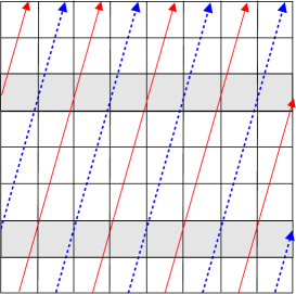
Figure 2: Schematic illustration of the ray-tracing scheme for the diffuse radiation in the two-dimensional mesh grid. For a given direction, equally-spaced parallel light-rays are cast from boundaries of the simulation volume and travel to the other boundaries. Note that gray mesh grids are traversed by multiple parallel light-rays, while the subsets of light-rays depicted by blue or red get through them only once.

2.3 Angular resolution for RT of the diffuse radiation

The number of the directions of light-rays, $N_{\rm d}$, determines angular resolution of the RT of the diffuse radiation. In order to guarantee that light-rays from a mesh grid on a face of the simulation box reach all the mesh grids on the other faces, $N_{\rm d}$ should be in the order of $N_{\rm m}^{2/3}$. In the case that the mean free path of the diffuse photons is sufficiently shorter the simulation box size, however, such a large $N_{\rm d}$ is redundant because only a small fraction of diffuse photons reach the other faces, and we can reduce the total computational cost by decreasing the number of directions, $N_{\rm d}$, while keeping the reasonable accuracy of the diffuse RT. Thus, the number of directions should be flexibly changed depending on the physical state.

To achieve this, we use the HEALPix (Hierarchical Equal Area isoLatitude Pixelization) software package (Górski et al., 2005) to set up the directions of the light-rays. The HEALPix is suitable to our purposes in the sense that each direction corresponds to exactly the same solid angle and that the directions are nearly uniformly sampled. Furthermore, it can provide a set of directions with these properties in arbitrary resolutions, each of which contains $12N_{\rm side}^{2}$ directions, where $N_{\rm side}$ is an angular resolution parameter. Since it is larger than the number of mesh grids on six faces of a cube with a side length of $N_{\rm side}$ mesh spacings, $6N_{\rm side}^{2}$, it is expected that a set of light-rays originated from a single point with directions generated by the HEALPix with an angular resolution parameter of $N_{\rm side}$ get through all the mesh grids within a cube centered by the point with a side length of $N_{\rm side}$ mesh spacings. Thus, the optimal number of directions should be chosen so that the mean free path of the recombination photons is sufficiently shorter than $N_{\rm side}\Delta H$, where $\Delta H$ is the mesh spacing.

2.4 Chemical reactions and radiative heating and cooling

With photo-ionization and photo-heating rates computed with the prescription described above, time evolutions of chemical compositions and thermal states of gas are computed in the same manner as adopted in Okamoto et al. (2012). Details of the numerical schemes are briefly described in appendices B,C and D.

The chemical reaction rates and radiative cooling rates adopted in this paper are identical to those adopted in Okamoto et al. (2012), and the literatures from which we adopt these rates are summarized in Table 1.

Table 1: Rates of chemical reactions and radiative cooling processes adopted in this paper. Reference for radiative recombination rates (RR) of HII, HeII and HeIII in the case-A and case-B approximation; collisional ionization rates (CIR) of HI, HeI, and HeII; recombination cooling rates (RCR) of HII, HeII and HeIII in the case-A and case-B approximation; collisional ionization cooling rates (CICR) of HI, HeI and HeII; collisional excitation cooling rates (CECR) of HI, HeI and HeII; bremsstrahlung cooling rate; inverse Compton cooling rate (CCR); photoionization cross sections (CS) of HI, HeI and HeII.

physical process	literature
RR (case-A)	(1), (1), (2)
RR (case-B)	(3), (3), (3)
CIR	(7), (7), (1)
RCR (case-A)	(2), (2), (2)
RCR (case-B)	(3), (5), (3)
CICR	(2), (2), (2)
CECR	(2), (2), (2)
BCR	(4)
CCR	(6)
CS	(8), (8), (8)

(1) Abel et al. (1997); (2) Cen (1992); (3) Hui & Gnedin (1997); (4) Hummer (1994); (5) Hummer & Storey (1998); (6) Ikeuchi & Ostriker (1986); (7) Janev et al. (1987); (8) Osterbrock (2006);

3 Implementation on Highly Parallel Architectures

In this section, we describe the details of the implementation of the RT calculation of the diffuse radiation which performs effectively on recently popular processors with highly parallel architecture, such as GPUs, multi-core CPUs, and many-core processors. Throughout this paper, we present the results using the implementation with the OpenMP and CUDA technologies. The former is supported by most of the multi-core processors, and the many-core processors such as the Intel Xeon-Phi processor, while the latter is the parallel programming platform for GPUs by NVIDIA.

In the implementation on GPUs with the CUDA platform, the fluid dynamical and chemical data in all the mesh grids are transferred from the memory attached to CPUs to those of GPUs prior to the RT calculations. After the RT calculations, ionization rates and heating rates in all the mesh grids computed on GPUs are sent back to the CPU memory.

3.1 Ray Grouping

In the calculations of the transfer of the diffuse radiation described in the previous section, many parallel light-rays travel from boundaries of the simulation volume until they reach the other boundaries. On processors with highly parallel architecture, a straightforward implementation is to assign a single thread to compute the RT along each light-ray and calculate the RT along multiple light-rays in parallel. Such a simple implementation, however, does not work because some mesh grids are traversed by multiple parallel light-rays (see gray mesh grids in Figure 2), and in computing equation (10), multiple computational threads write data to the identical memory addresses. Thus, equation (10) has to be computed not in parallel but in a exclusive manner using the “atomic operations”. The use of the atomic operations, however, significantly degrade the parallel efficiency and computational performance in many architectures.

To avoid such use of atomic operations and the deterioration of the parallel efficiency, we split the parallel light-rays into several groups so that parallel light-rays in each group do not traverse any mesh grid more than once. For example, in two-dimensional mesh grids in Figure 2, parallel light-rays are split into two groups each of which are depicted by blue and red arrows. One can see that light-rays in each groups do not intersect any mesh grids more than once. We can extend this technique to the three-dimensional mesh grids by splitting the parallel light-rays into four groups, where the light-rays in each group are cast from the two-dimensionally interleaved mesh grids as depicted by the same color in Figure 3.

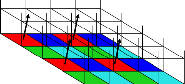
Figure 3: Schematic illustration of light-ray grouping for the three-dimensional mesh grids. Light-rays in each group start from boundary faces of mesh grids painted with the same color. Only the light-rays in one group are shown in this figure.

3.2 Efficient Use of Multiple External Accelerators

Many recent supercomputers are equipped with multiple external accelerators such as GPUs on a single computational node, each of which has an independent memory space. To attain the maximum benefit of the multiple accelerators, we decompose calculations of the diffuse radiation transfer according to the directions of the light-rays, and assign the decomposed RT calculation to the multiple accelerators. After carrying out the RT calculation for the assigned set of directions, and computing the mean intensity with equation (12) averaged over the partial set of directions on each external accelerator, the results are transferred to the memory on the hosting nodes. Then, we obtain the mean intensity averaged over all directions.

3.3 Node Parallelization

In addition to the thread parallelization within processors, we implement the inter-node parallelization using the Message Passing Interface (MPI). In the inter-node parallelization, the simulation box is evenly decomposed into smaller rectangular blocks with equal volumes along the Cartesian coordinate.

For the inter-node parallelization of the calculations of the diffuse radiation transfer, we adopt the multiple wave front (MWF) scheme developed by Nakamoto et al. (2001), in which light-ray directions are classified into eight groups according to signs of their three direction cosines, and for each group of light-ray directions, the RT calculations along each direction are carried out in parallel on a “wave front” in the node space, while the RT for different directions are computed on the other wave fronts simultaneously. By transferring the radiation intensities at the boundaries from upstream nodes to downstream ones, one can sequentially compute the RT of diffuse radiation along all the directions in each group of light-ray directions. See Nakamoto et al. (2001) for more detailed description of MWF scheme.

4 Test Simulation

In this section, we present a series of test simulations to validate our RT code. All the test simulations are carried out with $128^{3}$ mesh grids and the angular resolution parameter of $N_{\rm side}=8$ unless otherwise stated.

4.1 Test-1 : HII region expansion

The first test is the simple problem of a HII region expansion in a static homogeneous gas which consists of only hydrogen around a single ionizing source. We adopt the same initial condition as that of Test-2 in Cosmological Radiative Transfer Codes Comparison Project I (Iliev et al., 2006), where the hydrogen number density is $n_{\rm H}=10^{-3}\,{\rm cm}^{-3}$ and the initial gas temperature is $T=100\,{\rm K}$. The ionizing source emits the blackbody radiation with an effective temperature of $10^{5}\,{\rm K}$, and $5\times 10^{48}$ ionizing photons per second and located at a corner of simulation box with a side length of 6.6 kpc. In this initial condition, the recombination time is $t_{\rm rec}=122.4{\rm\,Myr}$ and the Strömgren radius is estimated to be 5.4 kpc. Figure 4 shows the radial profiles of ionization fraction and gas temperature at $t=30{\rm Myr}$, $100{\rm Myr}$ and $500{\rm Myr}$. The solid lines with and without circles indicate the results with and without the on-the-spot approximation (OTSA) , respectively. In the calculation with the effect of recombination radiation, the ionized regions are more extended than those computed with the on-the-spot approximation , especially at later stages ($t=100{\rm Myr}$ and $500{\rm Myr}$) because of the additional ionization of hydrogen by the recombination photons.

To verify the validity of our scheme for the transfer of diffuse recombination radiation, we compare our results with the ones obtained with the one-dimensional spherically symmetric RT code by Kitayama et al. (2004), which also incorporates the transfer of recombination photons emitted by the ionized hydrogen using the impact-parameter method. We find that the one-dimensional results with the effect of recombination radiation denoted by dashed lines show a good agreement with our three-dimensional results, indicating that our treatment of diffuse radiation transfer is consistent with that of well-established impact-parameter method.

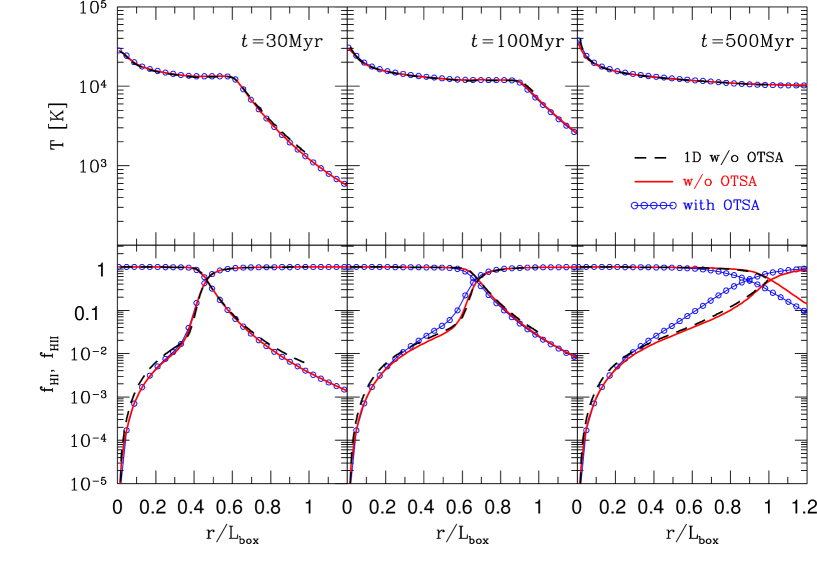
Figure 4: Test-1: Radial profiles of neutral and ionized fractions of hydrogen and gas temperature at $t=30{\rm Myr}$, $100{\rm Myr}$ and $500{\rm Myr}$. Solid lines with and without circles indicates the results with and without the on-the-spot approximation (OTSA), respectively. Dashed lines show the results obtained with one-dimensional spherically symmetric code without the OTSA presented in Kitayama et al. (2004).

4.2 Test-2 : Shadow by a dense clump

In the second test, we compute the RT from point radiation source in the presence of a dense gas clump. A point radiation source is located at the center of the simulation box with the same side length as the Test-1 (6.6kpc), and surrounded by the ambient uniform gas with the same hydrogen number density and temperature as the Test-1 ($n_{\rm H}=10^{-3}\,{\rm cm}^{-3}$ and $T=100\,{\rm K}$, respectively). In addition, we set up a spherical dense gas clump with a radius of 0.56 kpc centered at 0.8 kpc apart from the point radiation source along the $x$-direction. We set the density of the dense clump to 200 times higher than that of the ambient gas, and the temperature is set to 100 K. The spectrum and luminosity of the point radiation source is the same as that in Test-1.

In Figure 5, maps of the neutral fraction of hydrogen in the mid-plane of the simulation volume at $t=30\,{\rm Myr}$, 100Myr and 500Myr are shown. One can see that the ionizing photons are strongly absorbed by the dense gas clump and conical shadows are created behind the gas clump in the both runs with and without the effect of recombination radiation. In the run without the on-the-spot approximation (upper panels of Figure 5), the recombination photons emitted by the ionized gas gradually ionize the neutral gas behind the dense gas clump. On the other hand, in the run with the on-the-spot approximation, the boundaries of neutral and ionized regions are kept distinct because of the lack of recombination photons.

This test is identical to Test-6 in Hasegawa & Umemura (2010) calculated with the START code. In the START code, the RT is solved with a ray-tracing scheme based on the SPH technique, and the transfer of diffuse recombination radiation can be handled by allowing each SPH paricle to radiate recombination photons. Figure 7 shows profiles of gas temperature and hydrogen neutral fraction along the lines across the conical shadow shown in Figures 5 and 6 as well as the results obtained with the START code. One can see that both the results with and without the OTSA are in fairly good agreement with each other, which supports the validity of our scheme for diffuse radiation transfer.

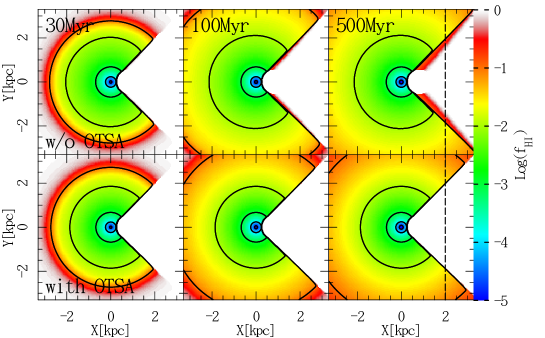
Figure 5: Test-2: Maps of neutral fraction of hydrogen in the mid-plane of the simulation box at $t=30{\,\rm Myr}$, $100{\,\rm Myr}$ and $500{\,\rm Myr}$. The lower and upper panels show the results with and without the on-the-spot approximation (OTSA), respectively. Dashed vertical lines indicate the location along which the profiles of temperature and neutral fractions are presented in Figure 7.

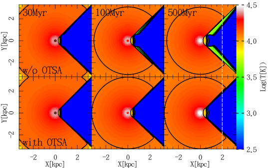
Figure 6: Test-2: Same as Figure 5 but shows the gas temperature maps in the mid-plane of the simulation box. Dashed vertical lines indicate the location along which the profiles of temperature and neutral fractions are presented in Figure 7.

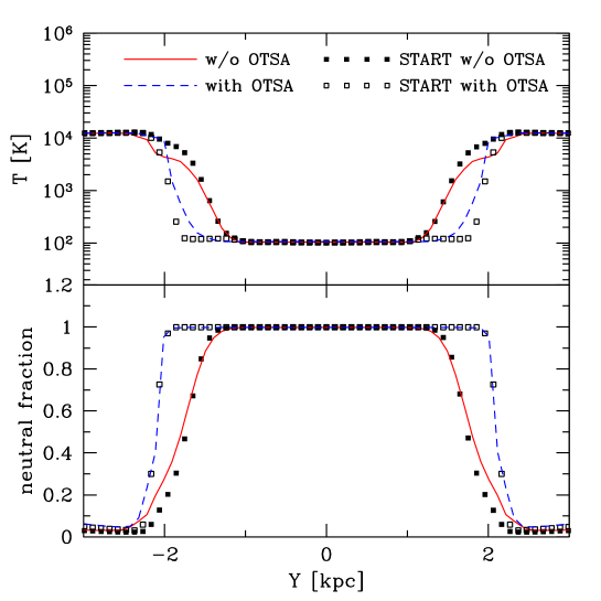
Figure 7: Profiles of temperatures and hydrogen neutral fractions along the dashed lines shown in Figures 5 and 6 with and without the OTSA. Results in Hasegawa & Umemura (2010) are also shown for comparison.

In this test, we also perform runs with various angular resolution parameter $N_{\rm side}$ in the RT calculation of diffuse radiation to see the effect of angular resolution. Figure 8 shows maps of neutral fraction of hydrogen in the mid-plane of the simulation box at $t=30\,{\rm Myr}$ with angular resolution parameter $N_{\rm side}$ of 16, 4 and 1. The results with $N_{\rm side}=16$ and $4$ are in good agreement with one with $N_{\rm side}=8$ in Figure 5, indicating that the angular resolution with $N_{\rm side}=4$ is sufficient for the current RT calculations. The results with $N_{\rm side}=1$, however, have spurious features in the map of neutral fraction. These numerical artifacts can be ascribed to the low angular resolution of light-rays by the comparison of the mean free path of the diffuse recombination photons and $N_{\rm side}\Delta H$. As described in § 4.2, the mean free path of the diffuse photons should be sufficiently smaller than $N_{\rm side}\Delta H$ to compute the RT of diffuse photons accurately. For the recombination photons emitted by ionized hydrogens in the current setup, the mean free path in the neutral ambient gas is estimated as

$$\lambda_{\rm mfp}=\frac{1}{n_{\rm HI}\sigma_{\rm HI}(\nu_{0})}=51.4\left(\frac{n_{\rm HI}}{10^{-3}{\rm cm}^{-3}}\right)^{-1}{\rm pc},$$ (24)

and the mesh spacing is $\Delta H=6.6{\,\rm kpc}/128=51.5{\,\rm pc}$. Thus, it is quite natural to have strong numerical artifacts in the results with $N_{\rm side}=1$, because the mean free path is almost equal to $N_{\rm side}\Delta H$, and the condition for the accurate RT calculation ($\lambda_{\rm mfp}\ll N_{\rm side}\Delta H$) is not satisfied.

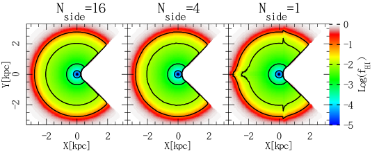
Figure 8: Test-2: Maps of neutral fraction of hydrogen in the mid-plane of the simulation box at $t=30{\,\rm Myr}$ for different angular resolution parameter, $N_{\rm side}=16$, 4 and 1 from left to right.

4.3 Test-3 : Ionization front trapping and shadowing by a dense clump

The third test computes the transfer of ionizing radiation incident to a face of the rectangular simulation box and the propagation of ionized region into a spherical dense clump. This test is indentical to the Test-3 in Iliev et al. (2006). The size of the simuation box is $6.6$ kpc, and hydrogen number density and initial temperature are set to $n_{\rm H}=2\times 10^{-4}$ cm^-3 and $T=8000$ K, except that a spherical dense clump with a radius of 0.8 kpc located at 1.7 kpc apart from the center of the simulation volume has a uniform hydrogen number density of $n_{\rm H,c}=200n_{\rm H}=0.04$ cm^-3 and a temperature of $T_{\rm c}=40$ K. The ionizing radiation has the blackbody spectrum with a tempearature of $T=10^{5}{\rm K}$ and constant ionizing photon flux of $F=10^{6}$ s^-1 cm^-2 at a boundary of the simulation box.

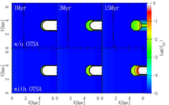
Figure 9: Test-3: Maps of neutral fraction of hydrogen in the mid-plane of the simulation box at $t=1$ Myr, 3 Myr and 15 Myr. The lower and upper panels show the results with and without the on-the-spot approximation, respectively.

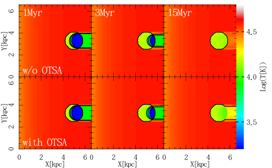
Figure 10: Test-3: Same as Figure 9 but shows the gas temperature maps in the mid-plane of the simulation box.

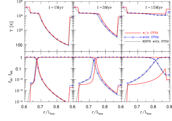
Figure 11: Test-3: Profiles of hydrogen neutral and ionized fractions and gas temperature along the axis of symmetry at $t=1$ Myr, 3 Myr and 15 Myr. Solid lines with and without circles indicate the results with and without the on-the-spot approximation, respectively. Dotted lines shows the results with RSPH code (Susa, 2006) presented in Iliev et al. (2006) with the on-the-spot approxiamtion.

Figures 9 and 10 shows the maps of hydrogen neutral fraction and gas temperature in the mid-plane of the simulation volume at $t=1$ Myr, 3 Myr and 15 Myr from left to right, where the ionizing photons enter from the left boundary of the figures. We show the results with and without the on-the-spot approximation in the lower and upper panels, respectively.

At $t=1$ Myr, the ionization front enters the spherical clump and a cylindrical shadow is formed behind the clump. At $t=3$ Myr and 15 Myr, the spherical clump is slightly ionized and the boundary of the shadow is ionized and photo-heated by the hard photons which penetrate the edge of the clump. These overall ionization and temperature structures with the on-the-spot approximation are consistent with the ones presented in Iliev et al. (2006). The effect of the recombination radiation is clearly seen in the results at 15 Myr, in which the cylindrical shadow is significantly ionized and heated by the recombination photons emitted at the ambient ionized region.

Figure 11 shows the profiles of ionized fraction and gas temperature along the axis of symmetry at $t=1$ Myr, 3 Myr and 15 Myr, where we also plot the results of the RSPH code (Susa, 2006) which are computed with the on-the-spot approximation and presented in Iliev et al. (2006). Our results with the on-the-spot approximation are consistent with the ones computed with the RSPH code in Iliev et al. (2006). The effect of the recombination radiation is siginificant at $t=3$ Myr and 15 Myr in the ionized fraction profiles, in which the recombination photons accelerate the propagation of the ionization front in the run without the on-the-spot approximation.

5 Performance

In this section, we show the performance of our RT calculations of diffuse radiation. The code for the transfer of diffuse radiation is designed so that it can be run both on multi-core CPUs and GPUs produced by NVIDIA. The performance is measured on the HA-PACS system installed in Center for Computational Sciences, University of Tsukuba. Each computational node of the HA-PACS system consists of two sockets of 2.6 GHz Intel Xeon processor E5-2670 with eight cores based on the Sandy-Bridge microarchitecture and four GPU boards of NVIDIA Tesla M2090, each of which is connected to the CPU sockets through PCI Express Gen2 $\times$ 16 link. Thus, a single computational node provides 2.99 Tflops (0.33 Tflops by CPUs and 2.66 Tflops by GPUs) of computing capability in double precision.

The upper panel of Figure 12 shows wallclock time for a iteration of the diffuse RT calculation on a single node with various numbers of CPU cores and GPU boards. The wallclock times are measured for $N_{\rm m}=64^{3}$, $128^{3}$ and $256^{3}$. The angular resolution parameter $N_{\rm side}$ is set to $N_{\rm side}=N_{\rm m}^{1/3}/16$ so that $N_{\rm side}\Delta H$ is kept constant. Note that the wallclock times are nearly proportional to $N_{\rm m}^{5/3}$ as theoretically expected. The lower panel of Figure 12 shows the performance gain of the diffuse RT calculation with multiple CPU cores and GPU boards relative to the performance with a single CPU core and a single GPU board, respectively. Use of the multiple CPU cores and multiple GPU boards provides the efficient performance gains nearly proportional to the adopted numbers of CPU cores and GPU boards for $N_{\rm m}=128^{3}$ and $256^{3}$ except for the fact that those with 16 CPU cores (2 CPU sockets) is not very impressive even for $N_{\rm m}=256^{3}$ because of the relatively slow memory access across the CPU sockets. On the other hand, the performance gain for $N_{\rm m}=64^{3}$ is somewhat degraded because of the overheads for invoking the multiple threads and communication overhead for data exchange between CPUs and GPUs. The performance with the aid of four GPU boards is nearly 7 times better than that with 16 CPU cores for $256^{3}$ mesh grids, while it is only 3.5 times better for $64^{3}$ mesh grids due to the communication overhead between CPUs and GPUs.

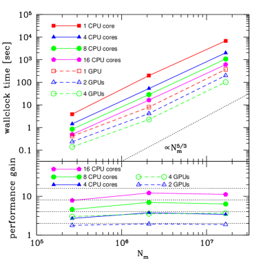
Figure 12: Wallclock times of diffuse RT calculation with various numbers of CPU cores and GPU boards for $N_{\rm m}=64^{3}$, $128^{3}$ and $256^{3}$ are shown in the upper panel. A dotted line indicate the dependence of computational cost on a number of mesh grids, $\propto N_{\rm m}^{5/3}$. In the lower panel, we present the performance gains of diffuse RT calculation with multiple CPU cores and GPU boards relative to the performance with a single CPU core and GPU board, respectively. Horizontal dotted lines indicates the performance gains of 2, 4, 8 and 16 from bottom to top.

We compare the performance of our diffuse RT calculations with and without the ray grouping technique on GPUs. In the implementation without the ray grouping technique, we utilize the atomic operation provided by the CUDA programming platform in computing the averaged radiation intensity (equation (11)). Figure 13 shows the performance gains obtained by the use of the ray grouping technique, where the individual performance is measured with a single computational node and four GPUs. One can see that the use of the ray grouping technique significantly improves the performance of diffuse RT more than by a factor of two irrespective of the number of mesh grids.

Figure 13: Performance gains obtained by the use of ray grouping for $N_{\rm m}=64^{3}$, $128^{3}$ and $256^{3}$ on GPUs. The performances are measured on a single computational node and four GPUs.

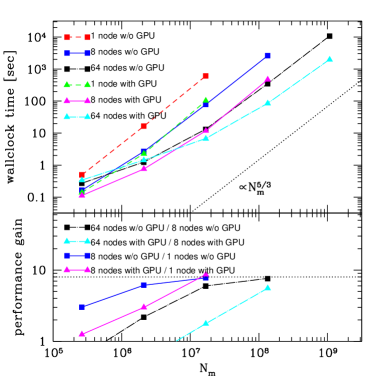
Figure 14: Wallclock times for diffuse RT calculation with various number of mesh grids computed with 1, 8 and 64 nodes are shown in the upper panel. The results with and without the use of four GPU boards are depicted. The dashed line indicates an analytic scaling of computational cost for the RT calculation of diffuse radiation, $N_{\rm m}^{5/3}$.

Figure 15: Upper panel: Wallclock times for MPI communication in diffuse radiation transfer calculations for various number of mesh grids with 8 and 64 nodes. A scaling relation of $N_{\rm m}^{4/3}$ is shown in a dashed line. Lower panel: fractions of wallclock times for MPI communication relative to total wallclock time elapsed in the calculations of diffuse radiation transfer in the runs with the use of GPUs.

The upper panel of Figure 14 shows the wallclock time of diffuse RT calculation performed on a single and multiple computational nodes with and without GPU boards, where we invoke one MPI process on each computational node. In the runs without the use of GPUs, each MPI process invokes 16 OpenMP threads, while in the runs with the aid of GPUs, we utilize four GPU boards on each computational node. We measure the wallclock time consumed for a single iteration of diffuse RT calculation for $64^{3}$–$1024^{3}$ mesh grids on 1, 8, and 64 computational nodes. The lower panel depicts the performance gain of the runs with 8 and 64 computational nodes relative to those with 1 and 8 computational nodes, respectively, where the ideal performance gain of 8 is shown by a dotted line. As for the runs without the use of GPUs, the parallel efficiency is reasonable when $N_{\rm m}/N_{\rm node}\geq 64^{3}$, where $N_{\rm node}$ is the number of computational nodes in use. For a given number of computational nodes, the runs with the use of GPUs have poorer performance gains than those without it, mainly beacause the computational times in the runs with GPUs are significantly shorter than those withtout GPUs, and the MPI data communication, as well as the commnication between CPUs and GPUs, gets more salient. Such communication overhead is proportional to the number of light-rays getting through the surface of the decomposed computational domains, $\propto N_{\rm m}^{2/3}N_{\rm d}\propto N_{\rm m}^{4/3}$. Figure 15 shows that the time consumed by the MPI communication is nearly proportional to $N_{\rm m}^{4/3}$, and that it occupies a significant fraction of the total wallclock time for a small $N_{\rm m}$. This scaling with respect to $N_{\rm m}$ has weaker dependence on $N_{\rm m}$ than the computational costs, $\propto N_{\rm m}^{5/3}$. Therefore, the overhead can be concealed for a sufficient number of mesh grids, and we have better parallel efficiency for a larger $N_{\rm m}/N_{\rm node}$.

6 Summary & Discussion

In this paper, we present a new implementation of the RT calculation of diffuse radiation field on three-dimensional mesh grids, which is suitable to be run on recent processors with highly-parallel architecture such as multi-core CPUs and GPUs. The code is designed to be run on both of ordinary multi-core CPUs and GPUs produced by NVIDIA by utilizing the OpenMP application programming interface and the CUDA programming platform, respectively.

Since our RT calculation is based on the ray-tracing scheme, the RT calculation itself can be carried out concurrently by assigning the RT calculation along each light-ray to individual software threads. To avoid the atomic operations in computing the averaged intensity (equation (10)) which can potentially degrade the efficiency of the thread parallelization, we devise a new scheme of the RT calculations in which a set of parallel light-rays are split into 4 groups so that parallel light-rays in each group do not get through any mesh grids more than once. As well as the thread parallelization inside processors or computational nodes, we also parallelize our code on a multi-node system using the MWF scheme developed by Nakamoto et al. (2001).

We perform several test simulations where the transfer of photo-ionizing radiation emitted by a point radiating source and recombination radiation from ionized regions as diffuse radiation are solved. We verify the validity of our RT calculation of the diffuse radiation by comparing our results with the effect of recombination radiation and the ones with other two independent codes, the one-dimensional spherical code by Kitayama et al. (2004) and START code by Hasegawa & Umemura (2010). We also clarify the condition of the required angular resolution in our diffuse radiation transfer scheme based on the mean free path of the diffuse photons and the mesh spacing.

We show good parallel efficiency of our implementation for intra- and inter-node parallelizations. As for the intra-node parallelization, the performance scales well with the number of CPU cores and GPU boards in use, except for the one in the case that multiple CPU sockets are used as a single shared-memory system. The scalability of the inter-node parallelization with the MWF scheme is also measured for $64^{3}$ to $1024^{3}$ mesh grids on up to 64 computational nodes and it is found that the inter-node parallelization is efficient when we have a sufficient number of mesh grids per node, $N_{\rm m}/N_{\rm node}\geq 128^{3}$ and $N_{\rm m}/N_{\rm node}\geq 64^{3}$ for the runs with and without GPUs, respectively. The ray-grouping technique described in 3.1 is effective and significantly improves the performance of our RT calculations by a factor of more than two, at least on GPUs (NVIDIA Tesla M2090).

With our implementation presented in this paper, we are able to perform the diffuse RT calculations in a reasonable wallclock time comparable to that of other physical processes such as hydrodynamical calculations. This means that the calculations of the diffuse radiation transfer can be coupled with hydrodynamic simulations and we are able to conduct radiation hydrodynamical simulations with the effect of diffuse radiation transfer as well as the radiation transfer from point radiating sources in three-dimensional mesh grids. Currently, we are developing such a radiation hydrodynamic code and, based on this, we will address astrophysical problems in which diffuse radiation transfer plays important roles.

It should be noted that, though we present the implementations and the performance on the multi-core CPUs and GPUs produced by NVIDIA, our approaches presented in this paper can be readily applied to other processors with similar architecture, such as the Intel Xeon-Phi processor or GPUs by other vendors. In addition, our approach can be easily extended to adaptively refined mesh grids using the prescription described in Razoumov & Cardall (2005), although we present the implementation for uniform mesh grids in this paper.

We would like to thank Tetsu Kitayama for providing us with his radiation transfer code. We are also grateful to the anonymous referee for helpful comments. Numerical simulations in this work have been carried out on the HA-PACS supercomputer system under the “Interdisciplinary Computational Science Program” in the Center for Computational Sciences, University of Tsukuba. This work was partially supported by Japan Society for the Promotion of Science (JSPS) Grant-in-Aid for Scientific Research (S) (20224002). TO acknowledges the financial support of JSPS Grant-in-Aid for Young Scientists (B: 24740112). KH acknowledges the support of MEXT SPIRE Field 5 and JICFuS and the financial support of JSPS Grain-in-Aid for Young Scientists (B: 24740114).

Appendix A Photon-conserving estimation of photo-heating and radiative cooling rates

We describe the photon-conserving evaluation of photo-ionization and photo-heating rates of a mesh grid contributed by a point radiating source, where the inner and outer intersections of a light-ray from the point raidating source and the mesh grid are located at $r_{\rm in}$ and $r_{\rm out}$ from the point radiating source. We consider a imaginary spherical shell centered at the point radiating source with inner and outer radii of $r_{\rm in}$ and $r_{\rm out}$, respectively. The incoming photon number per unit time $\dot{N}_{{\rm in},\nu}$ is given by

$$\dot{N}_{{\rm in},\nu}=\frac{L_{\nu}\exp(-\tau_{\nu})}{h\nu},$$ (25)

where $L_{\rm\nu}$ is the luminosity density at a frequency $\nu$, and $\tau_{\nu}$ is the optical depth between the point source and the inner side of the shell. The outgoing photon number per unit time from the outer side of the shell is written as

$$\dot{N}_{{\rm out},\nu}=\frac{L_{\nu}\exp(-(\tau_{\nu}+\Delta\tau_{\nu}))}{h\nu},$$ (26)

where $\Delta\tau_{\nu}$ is the radial optical depth of the shell. Then, the number of absorped photons per unit time $\dot{N}_{\rm abs}$ is given by

$$\dot{N}_{{\rm abs},\nu}=\dot{N}_{{\rm out},\nu}-\dot{N}_{{\rm in},\nu}=\frac{L_{\nu}\exp(-\tau_{\nu})}{h\nu}\left[1-\exp(-\Delta\tau_{\nu})\right].$$ (27)

When we consider multiple chemical components, the absoption rate of the $i$-th species is rewritten as

$$\dot{N}^{i}_{{\rm abs},\nu}=\frac{\Delta\tau^{i}_{\nu}}{\Delta\tau_{\nu}}\frac{L_{\nu}\exp(-\tau_{\nu})}{h\nu}\left[1-\exp(-\Delta\tau_{\nu})\right],$$ (28)

where $\Delta\tau^{i}_{\nu}$ is a optical depth contributed by the $i$-th component, and $\Delta\tau_{\nu}=\sum_{i}\Delta\tau^{i}_{\nu}$ is the total optical depth. Since $\dot{N}^{i}_{{\rm abs},\nu}$ is equal to the number of ionization of the $i$-th species, the photo-ionization rate of the $i$-th component can be written as

$$\Gamma_{i,\gamma}=\frac{1}{N_{i}}\int^{\infty}_{\nu_{i}}\dot{N}^{i}_{{\rm abs},\nu}d\nu,$$ (29)

where $\nu_{i}$ is the threshold frequecy of the $i$-th species and $N_{i}$ is the number of $i$-th species in the shell. The photo-heating rate is similarly calculated in terms of $\dot{N}_{{\rm abs},\nu}$ as

$${\cal H}_{i,\gamma}=\frac{1}{N_{i}}\int_{\nu_{i}}^{\infty}\dot{N}_{{\rm abs},\nu}(h\nu-h\nu_{i})d\nu.$$ (30)

Appendix B Ionization Balance

The time evolution of the number density of the $i$-th chemical species can be schematically described by

$$\frac{dn_{i}}{dt}=C_{i}(T,n_{j})-D_{i}(T,n_{j})n_{i},$$ (31)

where $C_{i}(T,n_{j})$ is the collective production rate of the $i$-th species and $D_{i}(T,n_{j})n_{i}$ is the destruction rate of the $i$-the species. For example, in the case of atomic hydrogen, $C_{\rm HI}$ and $D_{\rm HI}$ is given by

$$C_{\rm HI} = \alpha_{\rm HII}\,n_{\rm e}n_{\rm HII}$$ (32)

$$D_{\rm HI} = \Gamma_{\rm HI}n_{\rm e}+\Gamma_{\rm HI,\gamma}$$ (33)

where $\alpha_{\rm HII}(T)$ is the radiative recombination rate of HII, $\Gamma_{\rm HI}$ is the collisional ionization rate and $\Gamma_{\rm HI,\gamma}=\sum_{\alpha}\Gamma^{\alpha}_{\rm HI,\gamma}+\Gamma_{\rm HI,\gamma}^{\rm diff}$ is the photoionization rate of HI.

These equations are numerically solved using the backward difference formula (BDF) (Anninos et al., 1997; Yoshikawa & Sasaki, 2006), in which the number densities of the $i$-th chemical species at a time $t+\Delta t$, $n_{i}^{t+\Delta t}$, is computed as

$$n_{i}^{t+\Delta t}=\frac{C_{i}\Delta t+n_{i}^{t}}{1+D_{i}\Delta t},$$ (34)

where, $C_{i}$ and $D_{i}$ are estimated with the number densities of each species at the advanced time, $n_{j}^{t+\Delta t}$. However, the number densities in the advanced time step are not available for all the chemical species in evaluating $C_{i}$ due to the intrinsic non-linearity of equation 31. Thus, we sequentially update the number densities of each chemical species in the increasing order of ionization levels rather than updating all the species simultaneously. It is confirmed that this scheme is stable and accurate (Anninos et al., 1997; Yoshikawa & Sasaki, 2006).

Appendix C Photo-heating and radiative cooling

The specific energy change for each mesh by the photo-heating and radiative cooling is followed by the energy equation

$$\frac{du}{dt}=\frac{\mathcal{H}-\mathcal{C}}{\rho},$$ (35)

where $u$ is the specific internal energy and $\mathcal{H}$ and $\mathcal{C}$ are the photo-heating and cooling rate, respectively and $\mathcal{H}$ is given by

$$\mathcal{H}=\sum_{i}n_{i}\left(\sum_{\alpha}\mathcal{H}_{i}^{\alpha}+\mathcal{H}_{i}^{\rm diff}\right).$$ (36)

The specific internal energy for each mesh is updated implicitly by solving the equation

$$u^{t+\Delta t}=u^{t}+\frac{\mathcal{H}^{t+\Delta t}-\mathcal{C}^{t+\Delta t}}{\rho^{t}}\Delta t$$ (37)

for $u^{t+\Delta t}$, where the photo-heating $\mathcal{H}^{t+\Delta t}=\mathcal{H}(n^{t+\Delta t})$ and cooling rates $\mathcal{C}^{t+\Delta t}=\mathcal{C}(n^{t+\Delta t},u^{t+\Delta t})$ are evaluated at the advanced time $t+\Delta t$.

Appendix D Timestep constraints

Since we solve the static RT equation (1), equations (31) for chemical reactions and (35) for photo-heating and radiative cooling have to be solved iteratively until the electron number density and specific internal energy in each mesh grid converges: $|n_{\rm e}^{(i)}-n_{\rm e}^{(i-1)}|<\epsilon n_{\rm e}^{(i)}$ and $|u^{(i)}-u^{(i-1)}|<\epsilon u^{(i)}$, where $\epsilon$ is set to $10^{-3}$, and $n_{\rm e}^{(i)}$ and $u^{(i)}$ indicates the specific internal energy and the electron number density after the $i$-th iteration, respectively.

The timestep in solving chemical reactions and energy equation, $\Delta t_{\rm chem}$, is set to

$$\Delta t_{\rm chem}=\epsilon_{\rm e}\left|\frac{n_{\rm e}}{\dot{n}_{\rm e}}\right|+\epsilon_{\rm HI}\left|\frac{n_{\rm HI}}{\dot{n}_{\rm HI}}\right|,$$ (38)

where the second term on the right hand side prevents the timestep from getting prohibitively short in the case that the gas is almost neutral, and $\epsilon_{\rm e}$ and $\epsilon_{\rm HI}$ are set to 0.2 and 0.002, respectively.

The timestep, $\Delta t$, with which we update the radiation field can be larger than the chemical timestep, $\Delta t_{\rm chem}$ by subcycling the rate and energy equations (31) and (35). Throughout in this paper, the timestep for the RT calculation is set to

$$\Delta t=F\min_{i}\Delta t_{\rm chem,\it i},$$ (39)

where $\Delta t_{\rm chem,\it i}$ is the chemical timestep for the $i$-th mesh grid, and we typically set $F=1\sim 10$ so that the radiation field successfully converges with a reasonable number of iterations.

References

- Abel et al. (1997) Abel, T., Anninos, P., Zhang, Y., Norman, M. L., 1997, New Astronomy, 2, 181
- Abel, Norman & Madau (1999) Abel, T., Norman,M. L., Madau, P., 1999, ApJ, 523, 66
- Anninos et al. (1997) Anninos, P., Zhang, Y., Abel, T., Norman, M. L., 1997, New Astronomy, 2, 209
- Cen (1992) Cen, R., 1992, ApJS, 78, 341
- Ciardi et al. (2001) Ciardi, B., Ferrara, A., Marri, S., & Raimondo, G. 2001, MNRAS, 324, 381
- Dopita et al. (2011) Dopita, M. A., Krauss, L. M., Sutherland, R. S., Kobayashi, C., Lineweaver, C. H., 2011, Ap&SS, 335, 345
- Gnedin & Abel (2001) Gnedin, N. Y., Abel, T., 2001, New Astronomy, 6, 437
- González, Audit & Huynh (2007) González, M., Audit, E., Huynh, P., 2007, A&A, 464, 429
- Górski et al. (2005) Górski, K. M., Hivon, E., Banday, A. J., Wandelt, B. D., Hansen, F. K., Reinecke, M., Bartelmann, M., 2005, ApJ, 622, 759
- Hasegawa & Umemura (2010) Hasegawa, K., Umemura, M., 2010, MNRAS, 407, 2632
- Hui & Gnedin (1997) Hui, L., Gnedin, N. Y., 1997, MNRAS, 292, 27
- Hummer (1994) Hummer, D. G., 1994, MNRAS, 268, 109
- Hummer & Storey (1998) Hummer, D. G., Storey, P. J., 1998, MNRAS, 297, 1073
- Ikeuchi & Ostriker (1986) Ikeuchi, S., Ostriker, J. P., 1986, ApJ, 301, 522
- Iliev et al. (2006) Iliev, I. T. et al., 2006, MNRAS, 371, 1057
- Iliev et al. (2009) Iliev, I. T. et al., 2009, MNRAS, 400, 1283
- Inoue (2010) Inoue, A. K. 2010, MNRAS, 401, 1325
- Janev et al. (1987) Janev R. K., Langer W. D., Post Jr D. E., Evans Jr K., 1987, in Janev R.K., Lnger W.D., Evans, K., eds, Elementary Processes in Hydrogen-Helium Plasmas – Cross-section and Reaction Rate Coefficients. Springer-Verlag , Berlin
- Kanno et al. (2013) Kanno, Y., Harada, T., & Hanawa, T. 2013, PASJ, 65, 72
- Kitayama et al. (2004) Kitayama, T., Yoshida, N., Susa, H., Umemura, M., 2004, ApJ, 613, 631
- Kunasz & Auer (1988) Kunasz, P., Auer, L. H., 1988, J. Quant. Spectr. Radiative Transfer, 39, 67
- Miralda-Escudé (2003) Miralda-Escudé, J., 2003, ApJ, 597, 66
- Nakamoto et al. (2001) Nakamoto, T., Umemura, M., Susa, H., 2001, MNRAS, 321, 593
- Nakamoto et al. (2001b) Nakamoto, T., Umemura, M., & Susa, H. 2001, in ASP Conf. Ser. 222, The Physics of Galaxy Formation, ed. M. Umemura & H. Susa (San Francisco: ASP), 109
- Okamoto et al. (2012) Okamoto, T., Yoshikawa, K., Umemura, M., 2012, MNRAS, 419, 2855
- Okamoto et al. (2014) Okamoto, T., Shimizu, I., & Yoshida, N. 2014, PASJ, 66, 70
- Osterbrock (2006) Osterbrock, D. E., 2006, Astrophysics Of Gaseous Nebulae And Active Galactic Muclei. University Science Books
- Pawlik & Schaye (2011) Pawlik, A. H., Schaye, J., 2011, MNRAS, 412, 1943
- Rahmati et al. (2013a) Rahmati, A., Pawlik, A. H., Raičević, M., & Schaye, J. 2013, MNRAS, 430, 2427
- Rahmati et al. (2013b) Rahmati, A., Schaye, J., Pawlik, A. H., & Raičević, M. 2013, MNRAS, 431, 2261
- Razoumov & Cardall (2005) Razoumov, A. O., Cardall, C. Y., 2005, MNRAS, 362, 1413
- Rijkhorst et al. (2006) Rijkhorst, E.-J., Plewa, T., Dubey, A., Mellema, G., 2006, A&A, 452, 907
- Rosdahl et al. (2013) Rosdahl, J., Blaizot, J., Aubert, D., Stranex, T., & Teyssier, R. 2013, MNRAS, 436, 2188
- Skinner & Ostriker (2013) Skinner, M. A., & Ostriker, E. C. 2013, ApJS, 206, 21
- Sokasian et al. (2001) Sokasian, A., Abel, T., Hernquist, L. E., 2001, New Astronomy, 6, 359
- Stone et al. (1992) Stone, J. M., Mihalas, D., Norman, M. L., 1992, ApJS, 80, 819
- Susa (2006) Susa, H., 2006, PASJ, 58, 445
- Wise & Abel (2011) Wise, J. H., Abel, T., 2011, MNRAS, 414, 3458
- Wyithe et al. (2011) Wyithe, J. S. B., Mould, J., & Loeb, A. 2011, ApJ, 743, 173
- Yoshikawa & Sasaki (2006) Yoshikawa, K., Sasaki, S., 2006, PASJ, 58, 641