Uncertainty Quantification of the Pion-Nucleon Low-Energy Coupling Constants up to Fourth Order in Chiral Perturbation Theory

Abstract

We extract the statistical uncertainties for the pion-nucleon ($\pi N$) low energy constants (LECs) up to fourth order $\mathcal{O}(Q^{4})$ in the chiral expansion of the nuclear effective Lagrangian. The LECs are optimized with respect to experimental scattering data. For comparison, we also present an uncertainty quantification that is based solely on $\pi{}N$ scattering phase shifts. Statistical errors on the LECs are critical in order to estimate the subsequent uncertainties in ab initio modeling of light and medium mass nuclei which exploit chiral effective field theory. As an example of the this, we present the first complete predictions with uncertainty quantification of peripheral phase shifts of elastic proton-neutron scattering.

I Introduction

Chiral effective field theory ($\chi\mathrm{EFT}$) for nuclear physics provides a theoretical framework for a common description of various nuclear processes through the systematic generation of two- three- and many- body interactions and currents. Undoubtedly, it has allowed advances in ab initio structure calculations of light Maris et al. (2013) and medium mass Roth et al. (2012); Hergert et al. (2013); Hagen et al. (2012) atomic nuclei. The quantitative predictions of $\chi\mathrm{EFT}$ depend on the numerical values of a set of low-energy constants (LECs), which have become a limiting factor in medium mass nuclei where current sets of LECs fail to simultaneously predict binding, spectra, and radii. It is therefore relevant to constrain these LECs such that all predictions within the realm of applicability of $\chi\mathrm{EFT}$ can be quantified together with statistical uncertainties. This is important for advancing modern many-body calculations into regions of the nuclear chart and the physical processes where experimental data for verification is limited, such as neutrino-less double beta decay or structure and reactions near the neutron drip line. We present results that constrain the $\pi{}N$-sector of $\chi\mathrm{EFT}$, with accompanying confidence intervals (CI), up to fourth order in the expansion of the effective Lagrangian. At this order, the sub-leading long range three-nucleon interaction enters, and will thus be fully constrained by the results presented here. Further, many operator currents, such as the axial-vector current, depend on only $\pi{}N$ LECs and three nucleon contact LECs. Therefore careful uncertainty quantification of the $\pi{}N$ LECs is also critical for comparing processes driven by these currents to experimental cross sections and decay measurements.

The $\chi\mathrm{EFT}$ interaction Lagrangian $\mathcal{L}_{\rm eff}$ for atomic nuclei can be separated into two terms $\mathcal{L}_{\rm eff}=\mathcal{L}_{NN{}}+\mathcal{L}_{\pi{}N{}}$, and the two different contributions each depend explicitly on a distinctive set of LECs. The first term parametrizes the short-ranged contact-interactions and the second term describes the long-ranged and pion-mediated part of the two- and three-nucleon interaction. While the $NN$-contact sector must be constrained using nucleon-nucleon data, the LECs in $\mathcal{L}_{\pi{}N{}}$ can be determined from experimental $\pi{}N$ scattering-data, completely separately from the $NN$ terms. This is one example of how $\chi\mathrm{EFT}$ can link separate physical processes that are relevant for the description of atomic nuclei. Previous constraints for the $\pi{}N$ LECs have been determined from peripheral $NN$ scattering phase shifts Entem and Machleidt (2002); Ekström et al. (2013) or $\pi{}N$ elastic scattering phase shifts Büttiker and Meißner (2000); Fettes and Meißner (2000); Krebs et al. (2012). Indeed, these efforts have produced various sets of LECs that closely reproduce the respective phase shift analyses (either $NN$ Stoks et al. (1993); Arndt et al. (2007) or $\pi{}N$ Koch (1985, 1986); Workman et al. (2012); SAID online program solution WI08 ); however, the lack of reliable uncertainties on the input phase shifts prevents meaningful uncertainty quantification of the $\pi{}N$ LECs. It should be noted that available scattering phase shifts are not experientially measured data, but the result of a partial-wave analysis of measured data. In contrast with previous determinations of the $\pi{}N$ LECs, the analysis presented here is grounded in experimental scattering data. This allows us to estimate meaningful statistical uncertainties. For the first time we can therefore explore the consistency of $\chi\mathrm{EFT}$ by predicting CI’s for the peripheral $NN$ phase shifts determined by $\pi{}N$-data.

Table 1: Numerical values of the $\pi{}N$ LECs that result from the optimization with respect to explrimental observables. The resulting values are grouped from left to right in the order they appear in the Lagrangian.

$\mathcal{O}(Q^{1})$ LECs		$\mathcal{O}(Q^{2})$ LECs		$\mathcal{O}(Q^{3})$ LECs
[GeV-1]		[GeV-2]		[GeV-3]
$c_{1}$	$-1.40\,\pm\,0.12$	$\bar{d}_{1}+\bar{d}_{2}$	$+5.80\,\pm\,0.14$	$\bar{e}_{14}$	$+1.53\,\pm\,0.31$
$c_{2}$	$+1.71\,\pm\,0.33$	$\bar{d}_{3}$	$-5.66\,\pm\,0.08$	$\bar{e}_{15}$	$-11.91\,\pm\,0.87$
$c_{3}$	$-4.56\,\pm\,0.11$	$\bar{d}_{5}$	$+0.03\,\pm\,0.06$	$\bar{e}_{16}$	$+11.43\,\pm\,1.23$
$c_{4}$	$+3.72\,\pm\,0.27$	$\bar{d}_{14}-\bar{d}_{15}$	$-11.50\,\pm\,0.12$	$\bar{e}_{17}$	$+0.73\,\pm\,0.51$
				$\bar{e}_{18}$	$+0.57\,\pm\,1.36$

II Optimization

We seek a set of $\pi{}N$ LECs $\bm{c}_{\star}$ that minimize the least-squares objective function :

$$\chi^{2}_{\mathrm{red}}(\bm{c},\bm{N}) =\frac{1}{n_{df}}\left(\sum_{i}R_{i}(\bm{c},\bm{N})^{2}+\sum_{j}r_{i}(\bm{N})^{2}\right)$$ (1)

$$R_{i}(\bm{c},\bm{N}) =\frac{N_{j_{i}}O_{i}^{\chi\mathrm{EFT}{}}(\bm{c})-O_{i}^{\mathrm{Exp.}}}{\Delta_{i}^{Exp.}}$$ (2)

$$r_{j}(\bm{N}) =\frac{N_{j}-1}{\Delta_{j}}$$ (3)

where $O_{i}^{\chi\mathrm{EFT}{}}(\bm{c})$ denotes the value of the scattering observable computed from $\chi\mathrm{EFT}$, while $O_{ji}^{\mathrm{Exp.}}$ and $\Delta_{ji}^{Exp.}$ denotes the experimentally measured value and uncertainty, respectively, for the corresponding observable. $\bm{c}$ is a vector of LECs spanning all included $c_{i}$, $d_{i}$, and $e_{i}$ LECs. $\bm{N}$ is a vector of normalization coefficients $N_{j}$, where all points from a single experimental angular distribution share the same $N_{j}$; $\Delta_{j}$ encodes uncertainty of the experimental systematics for $N_{j}$. The number of degrees of freedom is given by $n_{\rm df}=(n_{d}+n_{N}-n_{NF})-(n_{\rm lecs}+n_{N})$, where $n_{d}$ is the number of data included in the fit, $n_{\rm lecs}$ is the number of LECs being fit, and $n_{N}$ is the number of unknown normalization coefficients and $n_{NF}$ is the number of floated coefficients (contribute no residual term in $r_{j}$ as $\delta_{j}=\infty$). For a given experiment $j$, the included data points run over a series of scattering angles at a fixed lab frame momentum $Q_{\rm Lab}$.

For our fitting dataset, we adopt the database from the most recent $\pi{}N$ partial wave analysis Workman et al. (2012), referred to as WI08. By construction, $\chi\mathrm{EFT}$ is a low-energy theory, therefore we exclude data with lab-frame momentum $Q_{\mathrm{Lab}}>160\,\mbox{MeV}$. This leaves us with an experimental database consisting of differential scattering cross-sections and polarization cross sections from $\pi^{\pm}+p\rightarrow\pi^{\pm}+p$ and $\pi^{-}+p\rightarrow\pi^{0}+n$ processes. In total, there are $n_{d}=1246$ data points, consisting of $1194$ differential unpolarized cross-sections and $52$ differential singly-polarized cross-sections. There are $n_{N}=110$ normalization coefficients, with $n_{NF}=9$ floated coefficients. There are other measurable observables, such as the spin rotation parameters, but experimental data only exists for momentum well beyond the range of validity of the EFT. The cutoff in lab frame momentum ($160\,\mbox{MeV}$) was chosen such that increasing or decreasing the cutoff would lead to a larger minimum value of $\chi^{2}_{\mathrm{red}}(\bm{c},\bm{N})$, maximizing amount of included data while avoiding fitting past the radius of convergence of the EFT.

For the calculated observables, we use the strong amplitudes presented in Ref. Krebs et al. (2012) (Refs. Fettes et al. (1998); Fettes (2000); Fettes and Meißner (2000, 2001) give a more complete presentation of the $\pi{}N$ scattering amplitudes, but use a different power counting scheme for relativistic corrections.) For the strong amplitude, we adopt their conventions for fixing $\bar{d}_{18}$, absorbing $\bar{e}_{19,20,21,22,35,36,37,38}$, $\bar{l}_{3}$ into $c_{1,2,3,4}$. We also work with exact isospin symmetry and use an averaged pion mass ($m_{\pi^{\vphantom{\pm}}}=(m_{\pi^{0}}+2m_{\pi^{\pm}})/3$). We adopt the electromagnetic treatment that is used in the WI08 partial wave analysis, which is described in detail inRefs. Tromborg et al. (1978); Tromborg and Hamilton (1974); Tromborg et al. (1977); Bugg (1973). For the electromagnetic corrections, we explicitly break isospin symmetry and use the physical pion masses within the coulomb amplitudes. Actual fits were performed using the TAO package Munson et al. (2012).

III Results

The central values and $1\sigma$ uncertainties of the $\pi{}N$ LECs up to fourth order in $\chi\mathrm{EFT}$ from fitting against scattering data are presented in Table 1. For this fit, we find that $\chi^{2}_{\mathrm{red}}=2.29$. As a comparison, the LECs from the fit against WI08 phase shifts of Ref. Krebs et al. (2012) generate $\chi^{2}_{\mathrm{red}}=3.63$ with respect to our objective function. Not surprisingly, our fit will reproduce experimental data better than the fits with respect to phase shifts. While our LECc are consistent with the spread of previous analyses, we find that no single analysis is entirely consistent with our fit at the $95\%$ confidence level, though the WI08 $\pi{}N$ phase shift fit from Ref. Krebs et al. (2012) lies just outside our interval.

Table 2: Covariance (lower triangle) and correlation (upper triangle) matrices for our fit to experimental data

LEC	$c_{1}$	$c_{2}$	$c_{3}$	$c_{4}$	$\bar{d}_{1}+\bar{d}_{2}$	$\bar{d}_{3}$	$\bar{d}_{5}$	$\bar{d}_{14}-\bar{d}_{15}$	$\bar{e}_{14}$	$\bar{e}_{15}$	$\bar{e}_{16}$	$\bar{e}_{17}$	$\bar{e}_{18}$
$c_{1}$	$+0.03$	$+0.95$	$+0.24$	$+0.56$	$+0.51$	$-0.33$	$-0.48$	$-0.45$	$-0.31$	$+0.37$	$-0.85$	$+0.15$	$-0.54$
$c_{2}$	$+0.07$	$+0.21$	$-0.08$	$+0.55$	$+0.54$	$-0.37$	$-0.48$	$-0.56$	$-0.32$	$+0.56$	$-0.96$	$+0.18$	$-0.54$
$c_{3}$	$+0.01$	$-0.01$	$+0.02$	$+0.13$	$-0.02$	$+0.12$	$-0.06$	$+0.26$	$+0.08$	$-0.58$	$+0.26$	$-0.12$	$-0.08$
$c_{4}$	$+0.03$	$+0.09$	$+0.01$	$+0.14$	$+0.97$	$-0.75$	$-0.77$	$-0.74$	$-0.39$	$+0.36$	$-0.55$	$+0.18$	$-0.94$
$\bar{d}_{1}+\bar{d}_{2}$	$+0.01$	$+0.05$	$-0.00$	$+0.07$	$+0.03$	$-0.81$	$-0.76$	$-0.75$	$-0.43$	$+0.46$	$-0.57$	$+0.18$	$-0.91$
$\bar{d}_{3}$	$-0.01$	$-0.02$	$+0.00$	$-0.03$	$-0.02$	$+0.01$	$+0.24$	$+0.67$	$+0.43$	$-0.45$	$+0.44$	$-0.24$	$+0.74$
$\bar{d}_{5}$	$-0.01$	$-0.02$	$-0.00$	$-0.02$	$-0.01$	$+0.00$	$+0.00$	$+0.52$	$+0.25$	$-0.28$	$+0.48$	$-0.04$	$+0.69$
$\bar{d}_{14}-\bar{d}_{15}$	$-0.01$	$-0.04$	$+0.01$	$-0.04$	$-0.02$	$+0.01$	$+0.01$	$+0.02$	$+0.34$	$-0.52$	$+0.62$	$-0.47$	$+0.81$
$\bar{e}_{14}$	$-0.02$	$-0.05$	$+0.00$	$-0.05$	$-0.03$	$+0.02$	$+0.01$	$+0.02$	$+0.13$	$-0.80$	$+0.50$	$-0.28$	$+0.41$
$\bar{e}_{15}$	$+0.07$	$+0.29$	$-0.10$	$+0.15$	$+0.10$	$-0.05$	$-0.02$	$-0.09$	$-0.33$	$+1.30$	$-0.76$	$+0.32$	$-0.40$
$\bar{e}_{16}$	$-0.22$	$-0.71$	$+0.06$	$-0.33$	$-0.17$	$+0.07$	$+0.05$	$+0.15$	$+0.30$	$-1.40$	$+2.59$	$-0.25$	$+0.56$
$\bar{e}_{17}$	$+0.01$	$+0.05$	$-0.01$	$+0.04$	$+0.02$	$-0.02$	$-0.00$	$-0.04$	$-0.06$	$+0.22$	$-0.24$	$+0.36$	$-0.50$
$\bar{e}_{18}$	$-0.14$	$-0.41$	$-0.02$	$-0.58$	$-0.27$	$+0.13$	$+0.08$	$+0.21$	$+0.24$	$-0.75$	$+1.48$	$-0.49$	$+2.70$

For uncertainty analysis, we apply a standard gradient expansion of $\chi^{2}(\bm{c})$ at the optimum $\bm{c}_{\star}$(see Ref. Dobaczewski et al. (2014) and references therein for further detail):

$$\chi^{2}(\bm{c})=\chi^{2}(\bm{c}_{\star})+\frac{1}{2}\sum_{a,b}\left(\bm{c}-\bm{c}_{\star}\right)_{a}\bm{H}_{a,b}\left(\bm{c}-\bm{c}_{\star}\right)_{b}+...\,,$$ (4)

$$\bm{H}_{a,b}=\frac{\partial^{2}\chi^{2}}{\partial c_{a}\partial c_{a}}\bigg{|}_{\bm{c}=\bm{c}_{\star}}\,,$$ (5)

where $\chi^{2}(\bm{c})$ is the full (not reduced by $n_{df}$) objective function. If the residual vectors ($R_{i}$ and $r_{j}$) are normally distributed, then the covariance matrix of our fit is given by

$$\bm{C}_{a,b}=\operatorname{cov}(c_{a}c_{b}) \approx\chi^{2}_{\mathrm{red}}\operatorname{inv}(\bm{H})_{a,b}\,,$$ (6)

$$\operatorname{corr}(c_{a}c_{b}) =\bm{C}_{a,b}/\sqrt{\bm{C}_{a,a}\bm{C}_{b,b}}\,.$$ (7)

.

The covariance matrix ($\bm{C}_{a,b}$) and correlation matrix $\operatorname{corr}(c_{a}c_{b})$ are presented in table 2.

Figure 1: $\pi{}N$ Observables computed at $\theta_{\rm c.m.}=45^{\circ}$. The blue (green) lines with diamond (square) markers show results for the $\pi{}^{+(-)}+p\rightarrow\pi{}^{+(-)}+p$ processes while the red lines with circular markers show the charge exchange process. The dashed lines show observables computed using our fit to experimental data. The dotted lines shows results reconstructed from LECs of Ref. Krebs et al. (2012). P is the polarization, while A and R are the spin rotation parameters, all presented as ratios with respect to the differential cross-section. Definitions of these observables can be found in Ref. Höhler (1983)

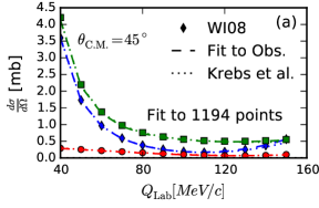
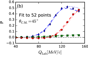
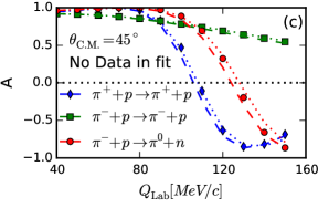
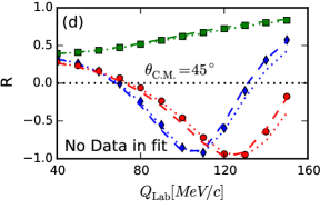
Figure 1 shows calculations of $\pi{}N$ scattering observables using our LECs fit data as well as LECs from the phase shift fit of Ref. Krebs et al. (2012). At smaller $Q_{\rm lab}$, the difference is minimal, but it is clear at higher momentum that phase shifts fits are inadequate. This is especially apparent in the calculations of the polarization (P) and spin rotation parameters (A and B), suggesting a phase shift fit may not adequately capture the underlying tensor effects that are critical to nuclear observables.

Figure 2: $\pi{}N$ phase shifts. The blue line is a prediction of our fit with the band showing the $95\%$ interval. For comparison, the red dotted lines are the phase shifts from Krebs et al. (2012). The markers show phase shifts from two partial wave analyses Koch (1985); Workman et al. (2012). The partial waves are denoted as [L][2I][2J] where L is the orbital angular momentum, I is the isospin, and J is the total angular momentum.

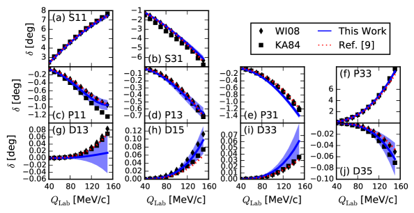
As a validation of our analysis, we plot $\pi{}N$ partial wave phase shifts in Fig. 2 and compare with two different partial wave analyses(WI08 Workman et al. (2012) and KA84 Koch (1985)) The blue bands denotes the $95\%$ CI from our fit. For S- and P-waves, we have good agreement with the WI08 partial wave analysis. In the D-waves, where the $\mathcal{O}(Q^{3})$ LECs have significant contributions, we find poor agreement in the $J=\tfrac{3}{2}$ channels (D13 and D33).

To better understand where this error in the $J=\tfrac{3}{2}$ D-waves is coming from, we can use the eigenstate of the covariance matrix to gain insight on the quality of the LEC constraints:

$$\bm{C}\bm{v}_{j} =\nu_{j}\bm{v}_{j}.$$ (8)

The vectors of LEC combinations, $\bm{v}_{j}$, form pseudo LECs that are completely uncorrelated, and eigenvalues $\nu_{j}$ are effective variances of these pseudo LECs. In table 3, we examine the LEC content of the least constrained eigenvectors (those with largest eigenvalue). It is clear that the largest eigenvectors are dominated by the $\bar{e}_{i}$ LECs, and in particular the pair $\bar{e}_{16}$, $\bar{e}_{18}$ which dominate the two most significant vectors. This indicates that $\bar{e}_{16}$ and $\bar{e}_{18}$ are poorly constrained. Within the scattering amplitudes, $\bar{e}_{16}$ and $\bar{e}_{18}$ span the non-spin-flip and spin-flip amplitudes respectively Krebs et al. (2012), suggesting that a lack of low momentum data for spin observables could be at fault.

Table 3: Eigenvalues ($\nu_{j}$) of the covariance matrix, with contributions to eigenvector ($v_{j}$) summed over LECs of same chiral order. These eigenvalue correspond to the variances $\sigma^{2}_{j}$ of effective uncorrelated pseudo LECs. For this analysis the covariance matrix was reduced to a dimensionless form using appropriate powers of the nucleon mass.

j	$\nu_{j}$	$\sum_{c_{i}}v^{2}_{j,c_{i}}$	$\sum_{\bar{d}_{i}}v^{2}_{j,\bar{d}_{i}}$	$\sum_{\bar{e}_{i}}v^{2}_{j,\bar{e}_{i}}$	$v^{2}_{j,\bar{e}_{16}}$	$v^{2}_{j,\bar{e}_{18}}$
1	4.1147	0.0525	0.0094	0.9382	0.3829	0.4207
2	1.4185	0.0362	0.0052	0.9587	0.2558	0.4798
3	0.5114	0.1067	0.0013	0.8920	0.2038	0.0038
4	0.2412	0.0748	0.0236	0.9016	0.0241	0.0157
5	0.0516	0.2721	0.0459	0.6819	0.0004	0.0021
6	0.0060	0.0076	0.9696	0.0227	0.0001	0.0044
7	0.0047	0.0134	0.9647	0.0220	0.0006	0.0008
8	0.0015	0.2194	0.6919	0.0887	0.0147	0.0368
9	0.0007	0.6323	0.2427	0.1250	0.0790	0.0002
10	0.0003	0.8666	0.0346	0.0987	0.0235	0.0348
11	0.0001	0.7617	0.0125	0.2258	0.0007	0.0007
12	0.0000	0.0080	0.9918	0.0002	0.0000	0.0000
13	0.0000	0.9488	0.0068	0.0444	0.0144	0.0001

IV Application to Uncertainty of $NN$ Phase Shifts

Accurate calculations accompanied with quantitative uncertainty estimates is of-course one of the principal goals of low-energy nuclear theory. This is critical to the study of nuclei near the neutron drip-line or for $0\nu\beta\beta$ decay where this insufficient data to validate many-body calculations.

As a first step towards quantifying the accuracy of the $\pi{}N$ sector of the $NN$ interaction, we will predict the confidence intervals of the peripheral ($J\geq 4$) $NN$ scattering phase shifts at $\textrm{N}^{3}\textrm{LO}$. These partial waves are fully determined by the long-ranged pion physics. It should also be noted that this is the first $\textrm{N}^{3}\textrm{LO}$ calculation of these phase shifts that is actually grounded in experimental scattering data.

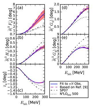
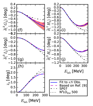
Figure 3 shows the predicted $95\%$ CIs of the proton- neutron elastic scattering phase shifts for all total angular momentum $J=4,5$ partial waves. For comparison, phase shifts from two different partial wave analyses are presented, PWA93 Stoks et al. (1993) and SP07 Arndt et al. (2007). We also compare to phase shifts computed using the high-precision Idaho-$\textrm{N}^{3}\textrm{LO}$ interaction Entem and Machleidt (2002), which reproduces the SM99 Machleidt (2001) $NN$ database with $\chi^{2}_{\mathrm{red}}\sim{}1$, and to $\textrm{N}^{3}\textrm{LO}$ $NN$ interactions computed using the LECs from Ref. Krebs et al. (2012). Our LECs perform quite favorably compared the $\pi{}N$ phase shift fit, and surprisingly favorable in many channels to the phase shifts computed from Idaho-$\textrm{N}^{3}\textrm{LO}$. For many channels, our error bands are remarkably small.

Figure 3: Elastic proton-neutron $J=4,5$ phase shifts at $\textrm{N}^{3}\textrm{LO}$ ($\Lambda=500$ MeV) with $95\%$ CIs from $\pi{}N$ data (red band). (Dotted line) the phase shifts from the $\textrm{N}^{3}\textrm{LO}$ interactions of Ref. Entem and Machleidt (2003). (Dashed line) the phase shifts from the Nijmegen partial wave analysis of Ref. Stoks et al. (1993).

V Conclusions

We constrained the $\pi{}N$ LECs using experimental data with $\chi^{2}/\textrm{datum}=2.29$, generating a set of LECs with error estimates that are compatible for use with modern $\textrm{N}^{3}\textrm{LO}$3 Hamiltonians and currents. We find that our lower order LECs are of natural size, while the higher order LECs tend to be unnaturally large (or small in the case of $\bar{d}_{5}$.) We find that even with fairly large error bars for some LECs, the proton-neutron peripheral phase shifts are very well constrained at lab scattering energies below $100\,\mbox{MeV}$. The $\pi{}N$ LECs not only fix the long range part of the $\textrm{N}^{3}\textrm{LO}$ three body force, but our analysis provides a means to examine uncertainty of the three body force in nuclear bound states as well as uncertainty from currents in observables. Progressing forward, simultaneous constraints of $\pi{}N$ and $NN$ LECs with quantitative statical analysis will yield predictions of few- and many-body systems with quantified uncertainty and is a topic for many future investigations.

VI Acknowledgments

The authors would like to thank H. Krebs, T. Papenbrock, D. Phillips, and R. Workman for their useful discussion. This work was supported in part by the U.S. Department of Energy (DOE) under Grant Nos. DEFG02-96ER40963 (University of Tennessee), DE-SC0008499 (NUCLEI SciDAC collaboration), Oak Ridge National Laboratory the Research Council of Norway under contract ISP-Fysikk/216699, and by the European Research Council under the European Community’s Seventh Framework Programme (FP7/2007-2013) ERC grant agreement no. 240603. Oak Ridge National Laboratory is supported by the DOE Office of Science under Contract No. DE- AC05-00OR22725.

References

- Maris et al. (2013) P. Maris, J. Vary, and P. Navrátil, Physical Review C 87, 014327 (2013), arXiv:0701038 [nucl-th] .
- Roth et al. (2012) R. Roth, S. Binder, K. Vobig, A. Calci, J. Langhammer, and P. Navrátil, Phys. Rev. Lett. 109, 052501 (2012).
- Hergert et al. (2013) H. Hergert, S. K. Bogner, S. Binder, a. Calci, J. Langhammer, R. Roth, and a. Schwenk, Phys. Rev. C 87, 034307 (2013).
- Hagen et al. (2012) G. Hagen, M. Hjorth-Jensen, G. R. Jansen, R. Machleidt, and T. Papenbrock, Physical Review Letters 109, 032502 (2012), arXiv:arXiv:1204.3612v1 .
- Entem and Machleidt (2002) D. R. Entem and R. Machleidt, Phys. Rev. C 66, 014002 (2002).
- Ekström et al. (2013) A. Ekström, G. Baardsen, C. Forssén, G. Hagen, M. Hjorth-Jensen, G. R. Jansen, R. Machleidt, W. Nazarewicz, T. Papenbrock, J. Sarich, and S. M. Wild, Physical Review Letters 110, 192502 (2013).
- Büttiker and Meißner (2000) P. Büttiker and U.-g. Meißner, Nuclear Physics A 668, 97 (2000).
- Fettes and Meißner (2000) N. Fettes and U.-G. Meißner, Nuclear Physics A 676, 311 (2000).
- Krebs et al. (2012) H. Krebs, A. Gasparyan, and E. Epelbaum, Physical Review C 85, 054006 (2012).
- Stoks et al. (1993) V. Stoks, R. Klomp, M. Rentmeester, and J. de Swart, Phys. Rev. C 48, 792 (1993).
- Arndt et al. (2007) R. Arndt, W. Briscoe, I. Strakovsky, and R. Workman, Phys. Rev. C 76, 025209 (2007).
- Koch (1985) R. Koch, Zeitschrift für Physik C Particles and Fields 29, 597 (1985).
- Koch (1986) R. Koch, Nuclear Physics A 448, 707 (1986).
- Workman et al. (2012) R. L. Workman, R. Arndt, W. J. Briscoe, M. W. Paris, and I. I. Strakovsky, Physical Review C 86, 035202 (2012).
- (15) SAID online program solution WI08, http://gwdac.phys.gwu.edu/analysis/pin_analysis.html.
- Note (1) See Refs. Arndt et al. (2007) for details on their process for a slightly older solution (SP06).
- Fettes et al. (1998) N. Fettes, U.-G. Meißner, and S. Steininger, Nuclear Physics A 640, 199 (1998).
- Fettes (2000) N. Fettes, Ann. Phys. 283, 273 (2000).
- Fettes and Meißner (2001) N. Fettes and U.-G. Meißner, Nuclear Physics A 693, 693 (2001).
- Tromborg et al. (1978) B. Tromborg, S. Waldenstrøm, and I. Øverbø, Helvetica Physica Acta 51 (1978), 10.5169/seals-114961.
- Tromborg and Hamilton (1974) B. Tromborg and J. Hamilton, Nuclear Physics B 76, 483 (1974).
- Tromborg et al. (1977) B. Tromborg, S. Waldenstrøm, and I. Øverbø, Physical Review D 15, 725 (1977).
- Bugg (1973) D. Bugg, Nuclear Physics B 58, 397 (1973).
- Munson et al. (2012) T. Munson, J. Sarich, S. Wild, S. Benson, and L. C. McInnes, TAO 2.0 Users Manual, Tech. Rep. ANL/MCS-TM-322 (Mathematics and Computer Science Division, Argonne National Laboratory, 2012) http://www.mcs.anl.gov/tao.
- Dobaczewski et al. (2014) J. Dobaczewski, W. Nazarewicz, and P.-G. Reinhard, Journal of Physics G: Nuclear and Particle Physics 41, 074001 (2014), arXiv:1402.4657 .
- Höhler (1983) G. Höhler, Pion Nucleon Scattering. Part 2: Methods and Results of Phenomenological Analyses, edited by H. Schopper, Landolt-Börnstein - Group I Elementary Particles, Nuclei and Atoms, Vol. 9b2 (Springer Berlin Heidelberg, Berlin, Heidelberg, 1983).
- Machleidt (2001) R. Machleidt, Phys. Rev. C 63, 024001 (2001).
- Entem and Machleidt (2003) D. R. Entem and R. Machleidt, Phys. Rev. C 68 (2003), 10.1103/PhysRevC.68.041001.