Quantum entanglement of two harmonically trapped dipolar particles

Abstract

We study systems of two identical dipolar particles confined in quasi one-dimensional harmonic traps. Numerical results for the dependencies of the entanglement on the control parameters of the systems are provided and discussed in detail. In the limit of a strong interaction between the particles, the occupancies and the von Neumann entropies of the bosonic and fermionic ground states are derived in closed analytic forms by applying the harmonic approximation. The strong correlation regimes of the system with the dipolar bosons and the system with the charged ones are compared with each other in regard to aspects of their entanglement.

1 Introduction

In recent years, the study of quasi one-dimensional (1D) systems of cold atoms with a short-range interaction has drawn considerable attention. In particular, an observation of the Tonks–Girardeau (TG) systems [1], where bosonic systems behave as gases of spinless non-interacting fermions [2], has inspired a great interest in exploring their properties. The recent technological developments have also opened up perspectives for the experimental realization of systems of spatially confined particles with long-range dipole–dipole interactions (DDI)[3, 4, 5, 6, 7], providing, among other things, new possibilities for studying quantum correlation effects in many-body systems. Since then, there has been a remarkable increase of interest in understanding the properties of such systems [8, 9, 10, 11, 12, 13]. For recent developments in studies of ultra-cold gases, including dipolar quantum gases, see the overview [14].

Also, the study of entanglement has attracted much attention within the last few years. Particularly the research activity has expanded towards investigating the entanglement properties in various systems composed of interacting particles. For instance, the recent studies include model systems such as the Moshinsky atom [15, 16, 17, 18], helium atoms and helium-like atoms [19, 20, 21], quantum dot systems [22, 23, 24, 25], and 1D systems of atoms interacting via a short-range contact interaction [26, 27, 28]. For details concerning the recent progress in entanglement studies of quantum composite systems, see [29]. However, according to our best knowledge, studies on the entanglement of dipolar particles have not yet drawn much attention. In this paper, we address this issue and gain some insight into the quantum entanglement properties of systems composed of two particles confined in a harmonic trap

$$V(\textbf{r})={m\over 2}(\omega^{2}x^{2}+\omega_{\bot}^{2}\rho^{2}),$$ (1)

with the DDI modeled by

$$U(\textbf{r})={d^{2}\over|\textbf{r}|^{3}}(1-3\mbox{cos}^{2}\theta_{rd}),$$ (2)

where $\mbox{cos}^{2}\theta_{rd}={\vec{r}\cdot\vec{d}/rd}$, and $d^{2}$ being the strength of the DDI. For the sake of simplicity, we focus here on the regime of strong anisotropy, $\epsilon=\omega_{\bot}/\omega>>1$. The theoretical description of such quasi-1D systems can be simplified, since one can assume that the particles stay in the lowest transverse confinement mode and the single-mode approximation (SMA) can be applied. Within this approximation, the system of four dipolar bosons in a trap of anisotropy of $\epsilon=50$ has recently been considered in [9], wherein the effects of the interaction strength on various characteristics (such as the density, the momentum distribution, and the occupation number distribution) have been determined.

For the two-particle system under consideration here, the Hamiltonian in the SMA is

$$H=\sum_{i=1}^{2}[-{1\over 2}{\partial^{2}\over\partial x_{i}^{2}}+{1\over 2}x_{i}^{2}]+gU(|x_{2}-x_{1}|).$$ (3)

with

$$U(x)=\epsilon^{3\over 2}(2\sqrt{\epsilon}x-e^{-{\epsilon x^{2}\over 2}}\sqrt{2\pi}(1+\epsilon x^{2})\mbox{erfc}({\sqrt{\epsilon\over 2}}x)),$$ (4)

where we have omitted the short-range contact interaction in order to explore only the pure dipolar effects (for details on this point, see, for example, [9]). The coordinates and the energies are measured in terms of $\sqrt{{m\omega}/{\hbar}}$, ${\hbar\omega}$, respectively, and the dimensionless coupling $g$ is related to the control parameters of the system by $g={d^{2}\sqrt{\omega}m^{3\over 2}(1+3\mbox{cos}2\theta)/8\hbar^{5\over 2}}$.

The system (3) has the convenient feature that the center of mass (cm.) and relative motion can be decoupled. In terms of

$$x={{x}_{2}-{x}_{1}\over\sqrt{2}},X={x_{1}+x_{2}\over\sqrt{2}},$$

the Hamiltonian (3) separates into $H=H^{x}+H^{X}$, where the cm. Hamiltonian $H^{X}=-{1/2}d^{2}_{X}+X^{2}/2$ is exactly solvable and the relative motion Hamiltonian is given by

$$H^{x}=-{1\over 2}{d^{2}\over dx^{2}}+{1\over 2}x^{2}+gU(\sqrt{2}|x|).$$ (5)

The Taylor expansion of $U(\sqrt{2}|x|)$ around $\epsilon=\infty$ gives ${\sqrt{2}|x|^{-3}}$, so that the relative motion is governed in the strictly 1D limit by

$$H^{\epsilon\rightarrow\infty}=-{1\over 2}{d^{2}\over dx^{2}}+{1\over 2}x^{2}+{g\sqrt{2}\over|x|^{3}}.$$ (6)

In this paper, we discuss the effect of both the anisotropy parameter $\epsilon$ and the interaction strength $g$ on the entanglement in the bosonic and fermionic ground states. Moreover, we derive, within the framework of the harmonic approximation (HA), closed form expressions for the natural orbitals and their occupancies in the $g\rightarrow\infty$ limit. Furthermore, using these results, we analytically calculate the corresponding asymptotic bosonic and fermionic von Neumann (vN) entropies and compare their values with the ones obtained numerically.

This paper is structured as follows. In Section 2, we discuss the entanglement characteristics of quasi-1D systems of two spinless identical particles. Section 3 is devoted to the results, and some concluding remarks are made in Section 4.

2 The measure of entanglement

The tool that is usually used to characterize quantum entanglement is the spectrum of the one-particle reduced density matrix (RDM) [31]. For systems of a quasi-1D geometry composed of two spinless particles, the RDM takes the form

$$\rho(x,x^{{}^{\prime}})=\int_{-\infty}^{\infty}\psi(x,y)\psi(x^{{}^{\prime}},y)dy.$$ (7)

The eigenvectors and eigenvalues of the RDM are sometimes called the natural orbitals and the occupancies, respectively, and we shall do the same. The normalization conditions for the occupancies of the bosonic $(+)$ and fermionic $(-)$ states give $\sum_{l}\lambda_{l}^{(+)}=1$, and $2\sum_{l}\lambda_{l}^{(-)}=1$, where the factor $2$ comes from the fact that the occupancies of the fermionic state are doubly degenerate. As discussed in [30], the state of two identical bosons is non-entangled only in two cases, i.e., when its Schmidt number (Sn) is $1$ or $2$, which corresponds to $\lambda_{i}^{(+)}=1$ and to $\lambda_{i}^{(+)}=\lambda_{j}^{(+)}=0.5$, respectively. As to a fermion state, it is non-entangled if, and only if, its total wavefunction can be expressed as one single determinant [30], which in turn corresponds to $\lambda_{i}^{(-)}=0.5$.

We will measure the amount of the entanglement via the vN entropy,

$$\mbox{S}_{vN}=\mbox{S}+\mbox{S}_{0},$$ (8)

where $\mbox{S}=-\mbox{Tr}[\rho\mbox{Log}_{2}\rho]$ is the ordinary vN entropy [31] and $\mbox{S}_{0}=0$ and $\mbox{S}_{0}=-1$ stand for the bosonic ($B$) and fermionic ($F$) states, respectively. In terms of the occupancies, we have $\mbox{S}_{B}=-\sum_{l=0}\lambda_{l}^{(+)}\mbox{log}_{2}\lambda_{l}^{(+)}$, $\mbox{S}_{F}=-1-2\sum_{l=0}\lambda_{l}^{(-)}\mbox{log}_{2}\lambda_{l}^{(-)}$. The measure (8) vanishes for the non-entangled points discussed above, except for the bosonic states with $\mbox{Sn}=2$, ($\mbox{S}_{B}=1$). As noted in the already cited [30], the vN entropy alone is insufficient to distinguish whether the bosonic state is entangled or not, since the following may happen: $\mbox{S}_{B}=1$ for the state with Sn different than $2$. For example, such a situation was observed in the system of bosons interacting via the short-range contact potential confined in a split trap [26].

3 Results and discussion

3.1 The weak-interaction limit

In the limit as $\epsilon\rightarrow\infty$ (the strictly 1D case) the system of bosons gets fermionized for any $g\neq 0$ [2], which is due to the singular behavior of the interaction potential $|x_{2}-x_{1}|^{-{3}}$ at $x_{1}=x_{2}$. In this limit, the two bosonic ground-state wavefunctions approach, as ${g\rightarrow 0}$, the modulus of the Slater determinant $\psi^{g\rightarrow 0}_{B}(x_{1},x_{2})=2^{-{1/{2}}}|\mbox{det}_{n=0,j=1}^{1,2}(\varphi_{n}(x_{j}))|$, where $\varphi_{n}$ are the single-particle orbitals of the ideal system ($g=0$). The above function is nothing else but a TG wavefunction, which means that the 1D dipolar bosons form a TG gas in the weak interaction regime. We have determined the value of the vN entropy associated with $\psi^{g\rightarrow 0}_{B}$ by calculating the occupancies numerically through a discretization technique (see, for example, [24]). The value obtained by us $\mbox{S}^{g\rightarrow 0}_{B}\approx 0.9851$ agrees well with that reported in [27] ($0.984$). On the other hand, in the non-interacting case $g=0$, the bosonic and fermionic ground-state wavefunctions are given by a simple product $\psi^{g=0}_{B}(x_{1},x_{2})=\varphi_{0}(x_{1})\varphi_{0}(x_{2})$ and a Slater determinant $\psi^{g=0}_{F}(x_{1},x_{2})=2^{-{1/{2}}}\mbox{det}_{n=0,j=1}^{1,2}(\varphi_{n}(x_{j}))$, respectively, and these states must be regarded as non-entangled (their corresponding vN entropies vanish). One can importantly conclude that the vN entropy of the fermionic ground-state is always continuous at $g=0$, which is in contrast to the vN entropy of the bosonic ground-state, which exhibits a discontinuity at this point as $\epsilon\rightarrow\infty$.

3.2 The strong-interaction limit

Now we come to the point where we explore the limit of $g\rightarrow\infty$ by use of a scheme developed in [24]. Due to the long-range nature of the DDI, the larger is $g$, the larger is the average distance between the particles. Hence, and because of the fact that the Taylor expansion of $U(\sqrt{2}|x|)$ around $|x|=\infty$ gives ${\sqrt{2}|x|^{-3}}$, one can conclude that at very large $g$ the distance between the particles is large enough so that the interaction among them does not depend on $\epsilon$. Thus, as long as we are interested in the regime when $g\rightarrow\infty$, we can focus only on Eq. (6).

To begin with, we expand the relative motion potential in (6), $V(x)=x^{2}/2+{g\sqrt{2}|x|^{-3}}$, around its local minimum $x_{c}=2^{1/10}(3g)^{1/5}$, retaining only the terms up to second order, $V(x)\approx V(x_{c})+{5}(x-x_{c})^{2}/2$. The relative motion Schrödinger equation with such a potential is of course exactly solvable and approximations to the lowest even ($+$) and odd ($-$) wavefunctions can be constructed as follows

$$\psi_{rel}^{(\pm)}=C^{(\pm)}(g)(e^{-{\sqrt{5}\over 2}(x-x_{c})^{2}}\pm e^{-{\sqrt{5}\over 2}(x+x_{c})^{2}}),$$ (9)

where $C^{(\pm)}(g)$ is the normalization factor that tends to ${5^{1\over 8}/\sqrt{2}{\pi}^{1\over 4}}$ as $g\rightarrow\infty$ both in the $(+)$ and $(-)$ case. After taking into account the cm. ground-state wavefunction,

$$\psi^{(\pm)}(x_{1},x_{2})=\psi_{rel}^{(\pm)}(x){e^{-{X^{2}\over 2}}\over\pi^{1\over 4}},$$

and then changing the variables back to $x_{1}$ and $x_{2}$, we obtain final forms of the approximations to the lowest total symmetric $(+)$ and antisymmetric $(-)$ wavefunctions as

$$\psi^{(\pm)}(x_{1},x_{2})=\zeta(x_{1},x_{2})\pm\zeta(x_{2},x_{1}),$$ (10)

with

$$\zeta(x_{1},x_{2})={C^{(\pm)}(g)\over\pi^{1\over 4}}e^{-{1\over 4}(x_{1}+x_{2})^{2}-{\sqrt{5}\over 2}({x_{2}-x_{1}\over\sqrt{2}}-x_{c})^{2}}.$$ (11)

Subsequently we translate the coordinates by $x_{1}\mapsto\tilde{x}_{1}-{x_{c}/\sqrt{2}},x_{2}\mapsto\tilde{x}_{2}+{x_{c}/\sqrt{2}}$, which turns Eq. (11) into $x_{c}$-independent form:

$$\tilde{\zeta}(\tilde{x}_{1},\tilde{x}_{2})={C^{(\pm)}(g)\over\pi^{1\over 4}}e^{-{1\over 4}(\sqrt{5}(\tilde{x}_{2}-\tilde{x}_{1})^{2}+(\tilde{x}_{1}+\tilde{x}_{2})^{2})}.$$ (12)

Due to the fact that the above function is symmetric under permutations of coordinates, it always has a Schmidt decomposition in the form [31]

$$\tilde{\zeta}(\tilde{x}_{1},\tilde{x}_{2})=\sum_{l=0}^{\infty}k_{l}v_{l}(\tilde{x}_{1})v_{l}(\tilde{x}_{2}),$$ (13)

where $\langle v_{k}|v_{l}\rangle=\delta_{kl}$. By changing the variables back in (13), namely, by $\tilde{x}_{1}\mapsto x_{1}+{x_{c}/\sqrt{2}},\tilde{x}_{2}\mapsto x_{2}-{x_{c}/\sqrt{2}}$, one arrives at $\zeta(x_{1},x_{2})=\sum_{l=0}^{\infty}k_{l}\mbox{L}_{l}(x_{1})\mbox{R}_{l}(x_{2})$, where the orbitals $\mbox{L}_{l}(x)=v_{l}(x+{x_{c}/\sqrt{2}});\mbox{R}_{l}(x)=v_{l}(x-{x_{c}/\sqrt{2}})$ satisfy $\langle\mbox{L}_{k}|\mbox{L}_{l}\rangle=\langle\mbox{R}_{k}|\mbox{R}_{l}\rangle=\delta_{kl}$. Finally, after substituting the expansions of $\zeta(x_{1},x_{2})$ and of $\zeta(x_{2},x_{1})$ into (10), we get

$$\psi^{(\pm)}(x_{1},x_{2})=\\ \sum_{l=0}^{\infty}k_{l}[\mbox{L}_{l}(x_{1})\mbox{R}_{l}(x_{2})\pm\mbox{R}_{l}(x_{1})\mbox{L}_{l}(x_{2})],$$

It is easy to infer that in the limit as $g\rightarrow\infty$, where $x_{c}\rightarrow\infty$, the integral overlap between the orbitals $\mbox{L}_{k}(x)$ and $\mbox{R}_{l}(x)$ vanishes for any $k,l$, $\langle\mbox{L}_{k}|\mbox{R}_{l}\rangle=0$. Hence, bearing in mind that $\langle\mbox{L}_{k}|\mbox{L}_{l}\rangle=\langle\mbox{R}_{k}|\mbox{R}_{l}\rangle=\delta_{kl}$, one can infer that the family $\{\mbox{L}_{l}(x)$, $\mbox{R}_{l}(x)\}$ forms asymptotically an orthonormal set as $g\rightarrow\infty$. In this limit the orbitals $\mbox{L}_{l}(x)$ and $\mbox{R}_{l}(x)$ are thus nothing else but the asymptotic natural orbitals with the occupancy $\lambda_{l}$ related to the corresponding coefficient $k_{l}$ by $\lambda_{l}=k_{l}^{2}$ (a two-fold degeneracy occurs). The bosonic and fermionic ground states have thus as $g\rightarrow\infty$ the same set of occupancies. Up to this point, our derivations are quite similar to those in [24], where the system of two Coulombically interacting particles was treated by the HA. Here we go one step further and derive closed form analytical expressions for the asymptotic occupancies and their natural orbitals basing on a methodology of [18], wherein a novel derivation of the occupancies of the analytically solvable two-particle Moshinsky model was given.

Following [18], we start with Mehler’s formula:

$$e^{-(u^{2}+v^{2}){z^{2}\over 1-z^{2}}+uv{2z\over 1-z^{2}}}=$$

$$=\sum_{l=0}^{\infty}\sqrt{1-z^{2}}({z\over 2})^{l}{\mbox{H}(l;u)\mbox{H}(l;v)\over l!},$$ (14)

where $\mbox{H}(l;.)$ is the $l^{th}$ order Hermite polynomial. Now it should be clear that the orbitals $v_{l}$ and their coefficients $k_{l}$ appearing in Eq. (13) can be found in closed forms by matching Eq. (12) with (14). Indeed, in the limit as $g\rightarrow\infty$ that we are interested in, only ($C^{(\pm)}(g)\rightarrow{5^{1\over 8}/\sqrt{2}{\pi}^{1\over 4}}$ in Eq. (12)), we arrive, after performing some tedious algebra, at

$$k_{l}^{g\rightarrow\infty}={\sqrt{{1-z^{2}}\over 2}z^{l}},$$

and

$$v_{l}^{g\rightarrow\infty}(\tilde{x})={w^{1\over 4}\over\pi^{1\over 4}\sqrt{2^{l}l!}}e^{-{1\over 2}w\tilde{x}^{2}}\mbox{H}(l;\sqrt{w}\tilde{x}),$$

where $z={(w-1)/(w+1)}$, $w=5^{1/4}$.

Next, using the analytical formula obtained above for $\lambda_{l}^{g\rightarrow\infty}$, $\lambda_{l}^{g\rightarrow\infty}=[k_{l}^{g\rightarrow\infty}]^{2}$, we compute the Rényi entropy [32], that is,

$$\mbox{S}_{R}^{g\rightarrow\infty}={1\over 1-q}\mbox{log}_{2}(2\sum_{l=0}^{\infty}[\lambda_{l}^{{}^{g\rightarrow\infty}}]^{q}),$$ (15)

where the factor $2$ comes from the normalization condition ($2\sum_{l=0}\lambda_{l}^{g\rightarrow\infty}=1$). It is easy to check that in the limit as $q\rightarrow 1$, Eq. (15) reduces to $\mbox{S}_{B}^{g\rightarrow\infty}=-2\sum_{l}\lambda_{l}^{{}^{g\rightarrow\infty}}\mbox{log}_{2}\lambda_{l}^{{}^{g\rightarrow\infty}}$. By performing the summation in (15), we get

$$\mbox{S}_{R}^{g\rightarrow\infty}={1\over 1-q}\mbox{log}_{2}({2^{1-q}(1-z^{2})^{q}\over 1-z^{2q}}),$$ (16)

and then, by taking the limit as $q\rightarrow 1$, we arrive at

$$\mbox{S}^{g\rightarrow\infty}_{B}={z^{2}\over z^{2}-1}\mbox{log}_{2}z^{2}-\mbox{log}_{2}(1-z^{2})+1,$$ (17)

$\mbox{S}^{g\rightarrow\infty}_{B}\simeq 1.24939$. As discussed in Section 2, the asymptotic fermionic and bosonic ground states share the same set of occupancies, so that the values of their vN entropies differ from each other only by one, $\mbox{S}^{g\rightarrow\infty}_{F}\simeq 0.24939$. In the next subsection we will confirm the correctness of our analytical results by comparing them with the results obtained numerically.

3.3 Numerical analysis

As far as we know, except for the cases discussed in the previous subsections, neither analytical solutions to Eq. (5) nor to Eq. (6) are known and we have to resort to numerical methods. Here we apply the Rayleigh–Ritz (RR) method, that uses as a variational trial function a linear combination of a finite set of some basis functions,

$$\phi(x)=\sum_{n=0}^{N-1}c_{n}u_{n}(x).$$ (18)

Since the interaction potential in Eq. (5), $U(\sqrt{2}|x|)$, is finite at the origin $x=0$, the basis of the harmonic oscillator (HO) eigenfunctions appears to be appropriate in this case. We found it to work well over the whole range of values of $\epsilon$ and $g$. On the other hand, when it comes to Eq. (6), the interaction potential in it, $\sim|x|^{-3}$, diverges at $x=0$, and the interaction integrals are not convergent in the HO basis. Fortunately, this divergence can be cured by using the pseudoharmonic oscillator basis [33]

$$u_{n}(x)\sim x^{\gamma-{1\over 2}}e^{-{1\over 2}x^{2}}{{}_{1}\mbox{F}_{1}}(-n;\gamma;x^{2}),$$ (19)

$0<x<\infty$, $(u_{n}(0)=0)$, where ${}_{1}\mbox{F}_{1}$ is the Kummer confluent hypergeometric function and $\gamma$ is a nonlinear parameter ($\gamma>{3/2}$), which, as we have verified, has a strong impact on the rate of the convergence of the RR method.

We determine the value of the parameter $\gamma$ according to an optimization strategy based on the stationarity of the trace of the RR matrix, $H^{RR}$ [34],

$$\frac{d}{d\gamma}\mbox{Tr}_{N}H^{RR}|_{\gamma=\gamma_{opt}}=0.$$ (20)

Having the RR wavefunctions $\phi_{i}(x)$ obtained in that way (where $\phi_{i}=0$ for $x<0$), we can construct the even $(+)$ and odd $(-)$ approximate solutions of (6) by putting $\psi^{(\pm)}_{i}\sim\phi_{i}(x)\pm\phi_{i}(-x)$.

For the demonstration of the convergence, Table 1 shows the numerical results for the ground-state energy of (6) together with the corresponding optimal values of $\gamma_{opt}$, for different values of $g$ and $N$. As can be seen, the convergence is fairly good over the full interacting regime, getting increasingly better with an increase in $g$. It is apparent from the results that the occurrence of the TG regime, which is manifested by the closeness of the relative energy value to $1.5$, takes place at a very small value of $g$, that is, at about $g=0.0001$.

$g$	$N$	$\gamma_{opt}$	$E_{0}^{(N)}(\gamma_{opt})$
$0.0001$	40	1.577	1.50333
	50	1.581	1.50330
$0.01$	40	1.940	1.58259
	50	1.960	1.58249
$1$	30	4.092	2.67084
	40	4.228	2.67079
$5$	20	5.942	3.98386
	30	6.240	3.98383
$1000$	5	30.37	24.6666
	10	31.29	24.6665

Table 1: The lowest approximate energy $E_{0}^{(N)}(\gamma_{opt})$ determined using the optimized RR method as discussed in the text.

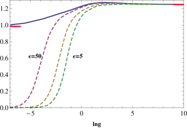
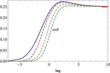
Figure 1: Upper figure: The dependence of the vN entropy of the bosonic ground-state on $\ln g$ for $\epsilon=5,10,50$ (dashed lines) and $\epsilon\rightarrow\infty$ (continuous line). The asymptotic values are marked by horizontal lines. Lower figure: Same as in upper figure but only for fermions.

Fig. 1 depicts our numerical results for the vN entropies of the bosonic and fermionic ground states calculated for some exemplary values of $\epsilon$, including the limiting case of $\epsilon\rightarrow\infty$. The numerical results for $\mbox{S}^{g\rightarrow 0}_{B}$ and the analytical ones for $\mbox{S}^{g\rightarrow\infty}_{B}$ and for $\mbox{S}^{g\rightarrow\infty}_{F}$ obtained in the previous subsections are marked by horizontal lines. As may be seen, the vN entropy increases, attains a local maximum, and then decreases, and in the limit of large $g$ saturates at a value that is insensitive to $\epsilon$. As a matter of fact, the last point has been already explained at the beginning of the subsection 3.2. As the figure indicates, our analytical results concerning the limit $g\rightarrow\infty$ are in excellent agreement with the numerical ones, which confirms their correctness and thereby proves the applicability of the HA to the case of dipolar particles. The dependence of the entanglement on $\epsilon$ is stronger in the bosonic case than in the fermionic one, which can be attributed to the fact that the probability of finding the bosons at the same place is, in contrast to fermions, affected by $\epsilon$ in particular. This effect is less pronounced at large $g$, where the bosons become spatially separated simulating thus the Pauli exclusion principle. Both in the bosonic and fermionic case, the vN entropy is largest in the 1D limit and its value attained in this limit by a local maximum is maximal. We see the TG regime starting to occur at a very small value of $g$, which is consistent with our earlier conclusion drawn from the numerical results for the relative motion energy (Table 1). When it comes to the points appearing in the behaviour of the bosonic vN entropy at which $\mbox{S}_{B}=1$, we have verified their Sn are essentially different from $2$, so they must be considered as truly entangled.

We close our discussion with a comparison of the present results obtained for the systems with the DDI with the ones obtained in [28] for quasi 1D systems of two harmonically trapped particles with a Coulomb interaction. Here we refer only to the strong correlation regimes of both systems, comparing them regarding their entanglement features. In particular, in [28], the value of the vN entropy of strongly interacting charged bosons was found to be about $1.14$. Comparing this value with that obtained in this paper, $\mbox{S}^{g\rightarrow\infty}_{B}\approx 1.25$, leads us to the conclusion that strongly interacting dipolar bosons are more entangled than the strongly interacting charged ones.

4 Summary

We carried out, within the single mode approximation (SMA), a comprehensive study of the entanglement properties of systems of two dipolar particles confined in a harmonic trap. Our results show the effect of the anisotropy parameter $\epsilon$ on the entanglement in the bosonic and fermionic ground states over the whole range of values of $g$. Moreover, within the framework of the harmonic approximation (HA), closed-form analytical expressions for the asymptotic natural orbitals and their occupancies have been obtained by use of Mehler’s formula. The corresponding vN entropies of the asymptotic bosonic and fermionic ground states have been also derived analytically and it has been shown that their values are in excellent agreement with the results obtained numerically.

References

- [1] T. Kinoshita, T. Wenger, and D. S. Weiss, Science 305 (2004) 1125
- [2] M. Girardeau, J. Math. Phys. 1 (1960) 516
- [3] A. Griesmaier et al., Phys. Rev. Lett. 94 (2005) 160401
- [4] C. Haimberger et al., Phys. Rev. A 70 (2004) 021402(R)
- [5] D. Tong et al., Phys. Rev. Lett. 93 (2004) 063001
- [6] C.-H. Wu, J. W. Park, P. Ahmadi, S. Will, and M. W. Zwierlein, Phys. Rev. Lett. 109 (2012) 085301
- [7] K.-K. Ni, S. Ospelkaus, M. G. H. de Miranda, A. Pe er, B. Neyenhuis, J. J. Zirbel, S. Kotochigova, P. S. Julienne, D. S. Jin, and J. Ye, Science 322 (2008) 231
- [8] S. Sinha and L. Santos, Phys. Rev. Lett. 99 (2007) 140406
- [9] F. Deuretzbacher, J. C. Cremon, and S. M. Reimann, Phys. Rev. A 81 (2010) 063616; Erratum Phys. Rev. A 81 (2010) 063616
- [10] S. Zöllner et al., Phys. Rev. Lett. 107 (2011) 035301
- [11] S. Zöllner, Phys. Rev. A 84 (2011) 063619
- [12] B. Chatterjee et al., J. Phys. B: At. Mol. Opt. Phys. 46 (2013) 085304
- [13] N. Bartolo et al., Phys. Rev. A 88 (2013) 023603
- [14] M. A. Baranov, al., Chem. Rev. 112 (2012) 5012-5061
- [15] R. Yañez, A. Plastino, and J. Dehesa, Eur. Phys. J. D 56 (2010) 141
- [16] A. Majtey, A. Plastino, and J. Dehesa, J. Phys. A: Math. Theor. 45 (2012) 115309
- [17] P. A. Bouvrie et al., Eur. Phys. J. D 66 (2012) 15
- [18] M. Glassera and I. Nagy, Physics Letters A 377 (2013) 2317
- [19] D. Manzano et al., J. Phys. A Math. Theor. 43 (2010) 275301
- [20] Y. Lin, C. Lin, and Y. Ho, Phys. Rev. A 87 (2013) 022316
- [21] G. Benenti, S. Siccardi, G. Strini, Eur. Phys. J. D (2013) 67
- [22] P. Kościk and H. Hassanabadi, Few-Body Systems 52 (2012) 189
- [23] R. G. Nazmitdinov et al., J. Phys. B: At. Mol. Opt. Phys. 45 (2012) 205503
- [24] P. Kościk and A. Okopińska Phys. Lett. A 374 (2010) 3841
- [25] A. V. Chizhov and R. G. Nazmitdinov, J. Phys.: Conf. Ser. 343 (2012) 012023
- [26] D. S. Murphy et al., Phys. Rev. A 76 (2007) 053616
- [27] B. Sun, D. L. Zhou, and L. You, Phys. Rev. A 73, (2006) 012336
- [28] P. Kościk, Few-Body Systems 52 (2012) 49
- [29] M. Tichy, F. Mintert, and A. Buchleitner, J. Phys. B: At. Mol. Opt. Phys. 44 (2011) 192001
- [30] G. Ghirardi and L. Marinatto Phys. Rev. A 70 (2004) 012109
- [31] R. Paškauskas and L. You, Phys. Rev. A 64 (2001) 042310
- [32] A. Rényi, Probability Theory, North-Holland, Amsterdam, 1970
- [33] R. L. Hall and N. Saad, J. Phys. A 33 (2000) 569
- [34] A. Okopińska Phys. Rev. D 36 (1987) 1273