Knowledge-Based Automatic Generation
of Partitioned Matrix Expressions

Abstract

In a series of papers it has been shown that for many linear algebra operations it is possible to generate families of algorithms by following a systematic procedure. Although powerful, such a methodology involves complex algebraic manipulation, symbolic computations and pattern matching, making the generation a process challenging to be performed by hand. We aim for a fully automated system that from the sole description of a target operation creates multiple algorithms without any human intervention. Our approach consists of three main stages. The first stage yields the core object for the entire process, the Partitioned Matrix Expression (PME), which establishes how the target problem may be decomposed in terms of simpler sub-problems. In the second stage the PME is inspected to identify predicates, the Loop-Invariants, to be used to set up the skeleton of a family of proofs of correctness. In the third and last stage the actual algorithms are constructed so that each of them satisfies its corresponding proof of correctness. In this paper we focus on the first stage of the process, the automatic generation of Partitioned Matrix Expressions. In particular, we discuss the steps leading to a PME and the knowledge necessary for a symbolic system to perform such steps. We also introduce Cl1ck, a prototype system written in Mathematica that generates PMEs automatically.

1 Introduction

In the context of the Formal Linear Algebra Methods Environment (FLAME) project [1], a methodology for the systematic derivation of algorithms for matrix operations has been developed and demonstrated. The approach has been successfully applied to all the operations included in the BLAS [2] and RECSY [3, 4] libraries and to many included in the LAPACK [5] library. In general, the methodology applies to any operation that can be expressed in a “divide and conquer” fashion. As opposed to the concept of “Autotuning”, which indicates the automatic tuning of a given algorithm [6, 7, 8], the word derivation refers to the actual generation of both algorithms and routines to solve a given target equation [9]. The remarkable results achieved using this methodology are the subject of a series of publications. a) For many standard operations, e.g. the Cholesky and the LU factorizations, all the previously known algorithms were systematically discovered, unifying them under a common root [10]. b) For more involved operations like the Sylvester equation and the reduction of a generalized eigenproblem to standard form, the generated family of algorithms included new and better performing ones [11, 12]. c) A related methodology for systematic analysis of round-off errors yielded bounds tighter than those previously known [13].

Although successful, the approach presents some limitations. The algorithms are generated through complex symbolic computations, steps often too complicated to be carried out by hand. Motivated by these difficulties, we aim for a symbolic system that, given as input the description of a matrix equation $Eq$, applies the steps dictated by the FLAME methodology to derive a family of algorithms to solve $Eq$. As shown in Fig. 1, the procedure consists of three successive stages—PME Generation, Loop-Invariant Identification, Algorithm Derivation—and is entirely determined by the mathematical description of the input operation.

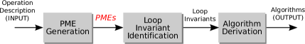
Figure 1: The three main stages in the process of derivation of algorithms.

In the first stage, the Partitioned Matrix Expression (PME) for the input operation is obtained. A PME is a decomposition of the original problem into simpler sub-problems in a “divide and conquer” fashion, exposing the computation to be performed in each part of the output matrices. An example is shown in Box 1. The second stage of the process deals with the identification of Boolean predicates, the Loop-Invariants, that describe the intermediate state of computation for the sought-after algorithms. Loop-invariants can be extracted from the PME, and are at the heart of the automation of the third stage. In the third and last stage of the methodology, each loop-invariant is used to set up a proof of correctness around which the algorithm is finally built. Notice that the objective is not proving the correctness of a given algorithm; vice-versa, the loop-invariant is chosen before the algorithm is built. Indeed, the algorithm is constructed to satisfy a given proof of correctness, i.e., to possess the chosen loop-invariant.

$\left({\begin{array}[]{@{}c@{}}X_{T}=\Omega(L_{TL},U,C_{T})\\ \hline\cr X_{B}=\Omega(L_{BR},U,C_{B}-L_{BL}X_{T})\end{array}}\right)$

Box 1 Partitioned Matrix Expression for the triangular Sylvester equation.

This paper centers around the first stage of the derivation process, the generation of PMEs. To this end we introduce a formalism to input into the system the minimum amount of knowledge about the operation required by a system to perform all the subsequent stages automatically. We then describe the process for transforming an input equation into PMEs. As Fig. 2 shows, such process involves three steps: 1) the partitioning of the operands in the equation, 2) matrix arithmetic involving the partitioned operands, and 3) a sequence of iterations, each consisting of algebraic manipulation and pattern matching. We demonstrate that the process can indeed be automated through Cl1ck, a symbolic system written in Mathematica [14] that performs all the steps for the PME generation.

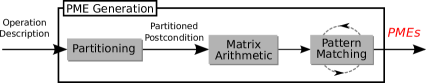
Figure 2: Steps for the automatic generation of PMEs.

The paper is organized as follows. In Sect. 2 we categorize the input needed by a symbolic system. Partitionings of the operands and inheritance of properties are discussed in Sect. 3, while in Sect. 4 we describe how to use partitionings to obtain PMEs. We draw conclusion in Sect. 5.

2 Input to the System

Our first concern is to establish how a target operation should be formally described. Since we are aiming for a fully-automated system, i.e., without any human intervention, we need a formalism to unequivocally describe a target equation. We choose the language traditionally used to reason about program correctness: equations shall be specified by means of the predicates Precondition ($P_{\rm pre}$) and Postcondition ($P_{\rm post}$) [15]. The precondition enumerates the operands that appear in the equation and describes their properties, while the postcondition specifies the equation to be solved.

The Cholesky factorization will serve as an example: given a symmetric positive definite (SPD) matrix $A$, the goal is to find a lower triangular matrix $L$ such that $LL^{T}=A$. Box 2 contains the predicates $P_{\rm pre}$ and $P_{\rm post}$ relative to the Cholesky factorization; the notation $L=\Gamma(A)$ indicates that $L$ is the Cholesky factor of $A$.

$$\small L=\Gamma(A)\equiv\left\{\begin{split}P_{\rm pre}:\{&{\tt{Unknown(}}L{\tt{)}}\;\wedge\;{\tt{LowerTriangular(}}L{\tt{)}}\;\;\wedge\\ &{\tt{Known(}}A{\tt{)}}\;\wedge\;{\tt{SPD(}}A{\tt{)}}\}\\ \\[-11.38109pt] P_{\rm post}:\{&LL^{T}=A\}\end{split}\right.$$

Box 2 Formal description for the Cholesky factorization.

Even though such a definition is unambiguous, it does not include all the information needed by a symbolic system to fully automate the derivation process. In Sect. 2.1 we discuss how a system expands its knowledge by “learning of” new equations, and in Sect. 3 we overview the ground knowledge that a system must possess relative to matrix partitioning and inheritance of properties.

2.1 Pattern Learning

We refer to the pair of predicates ($P_{\rm pre}$ and $P_{\rm post}$) in Box 2 as the pattern that identifies the Cholesky factorization. Such a pattern establishes that matrices $L$ and $A$ are one the Cholesky factor of the other provided that the constraints in the precondition are satisfied, and $L$ and $A$ are related as dictated in the postcondition ($LL^{T}=A$). For instance, in the expression

$$XX^{T}=A-BC,$$

in order to determine whether $X=\Gamma(A-BC)$, the following facts need to be asserted: i) $X$ is an unknown lower triangular matrix; ii) the expression $A-BC$ is a known quantity ($A,B$ and $C$ are known); iii) the matrix $A-BC$ is symmetric positive definite.

The strategy for decomposing an equation in terms of simpler problems greatly relies on pattern matching. In the next section we describe how matrix equations can be rewritten in terms of sub-matrices, resulting in expressions seemingly more complicated than the initial formulation. Such expressions are thus inspected to find segments corresponding to known patterns.

Initially, Cl1ck only knows the patterns for a basic set of operations: addition, multiplication, inversion, and transposition of matrices, vectors and scalars. This information is hard-coded. More complex patterns are instead discovered during the process of PME generation. For instance, the first time the PME for the Cholesky factorization is generated, Cl1ck learns and stores the pattern specified by Box 2. Thanks to such patterns it will then be possible to identify that a Cholesky factorization may be decomposed into a combination of triangular systems and simpler Cholesky factorizations. As Cl1ck’s pattern knowledge increases, also does its capability of tackling complex operations.

3 Partitioning and Inheritance

In this section we illustrate the first step towards the PME generation: the partitioning of the operands (Fig. 2). To this end we introduce a set of rules to partition and combine operands and to assert properties of expressions involving sub-operands. The application of these rules to the postcondition yields a predicate called partitioned postcondition. Due to constraints imposed by both the structure of the input operands and the postcondition, only few partitioning rules will be admissible.

3.1 Operands Partitioning and Direct Inheritance

As shown in Box 3, a generic matrix $A$ can be partitioned in four different ways. The $1\times 1$ rule (Box 3LABEL:sub@sbox:part1x1) is special as it does not affect the operand; we refer to it as the identity. For a vector, only the $2\times 1$ and $1\times 1$ rules apply, while for scalars only the identity is admissible. When referring to any of the parts resulting from a non-identity rule, we use the terms sub-matrix or sub-operand, and for $2\times 2$ partitionings we also use the term quadrant.

$\begin{aligned} A_{m\times n}\rightarrow&\left(\begin{array}[]{@{}c@{\,}|@{\,}c@{}}A_{TL}&A_{TR}\\ \hline\cr A_{BL}&A_{BR}\end{array}\right)\\ \small\textnormal{where }&A_{TL}\textnormal{ is }k_{1}\times k_{2}\end{aligned}$

(a) $2\times 2$ rule

$\begin{aligned} A_{m\times n}\rightarrow&\left(\begin{array}[]{@{}c@{}}A_{T}\\ \hline\cr A_{B}\end{array}\right)\\ \small\textnormal{where }&A_{T}\textnormal{ is }k_{1}\times n\end{aligned}$

(b) $2\times 1$ rule

$\begin{aligned} A_{m\times n}\rightarrow&\left(\begin{array}[]{@{}c@{\,}|@{\,}c@{}}A_{L}&A_{R}\end{array}\right)\\ \small\textnormal{where }&A_{L}\textnormal{ is }m\times k_{2}\end{aligned}$

(c) $1\times 2$ rule

$\begin{aligned} A_{m\times n}\rightarrow&\left(\begin{array}[]{@{}c@{}}A\end{array}\right)\\ \small\textnormal{where }&A\textnormal{ is }m\times n\end{aligned}$

(d) $1\times 1$ (identity) rule

Box 3 Rules for partitioning a generic matrix operand A. We use the subscript letters $T$, $B$, $L$, and $R$ for $T$op, $B$ottom, $L$eft, and $R$ight, respectively.

The inheritance of properties plays an important role in subsequent stages of the algorithm generation process. Thus, when the operands have a special structure, it is beneficial to choose partitioning rules that respect the structure. For a symmetric matrix, for instance, it is convenient to create sub-matrices that exhibit the same property. The $1\times 2$ and $2\times 1$ rules break the structure of a symmetric matrix, as neither of the two sub-matrices inherit the symmetry. Therefore, we only allow $1\times 1$ or $2\times 2$ partitionings, with the extra constraint that the $TL$ quadrant has to be square.

Box 4 illustrates the admissible partitionings for symmetric matrices. On the left, the identity rule is applied and the operand remains unchanged. On the right instead, a constrained $2\times 2$ rule is applied, so that some of the resulting quadrants inherit properties. Both $M_{TL}$ and $M_{BR}$ are square and symmetric, and $M_{BL}=M_{TR}^{T}$ (or vice versa $M_{TR}=M_{BL}^{T}$). Each matrix type allows specific partitioning rules and inheritance of properties; for triangular, diagonal, symmetric, and SPD matrices a library of admissible partitioning rules is incorporated into Cl1ck.

$\begin{aligned} M_{m\times m}\rightarrow&\left(\begin{array}[]{@{}c@{}}M\end{array}\right)\\ \small\textnormal{where }&M\textnormal{ is }m\times m\end{aligned}$  or

$\begin{aligned} M_{m\times m}\rightarrow&\left(\begin{array}[]{@{}c@{\,}|@{\,}c@{}}M_{TL}&M_{BL}^{T}\\ \hline\cr M_{BL}&M_{BR}\end{array}\right)\\ \small\textnormal{where }&M_{TL}\textnormal{ is }k\times k\end{aligned}$

Box 4 Partitioning rules for structured matrices.

3.2 Theorem-aware Inheritance

Although frequent, direct inheritance of properties is only the simplest form of inheritance. Here we expose a more complex situation. Let A be an SPD matrix. Because of symmetry, the only admissible partitioning rules are the ones listed in Box 4; applying the $2\times 2$ rule, we obtain

$$\begin{aligned} A_{m\times m}\rightarrow&\left(\begin{array}[]{@{}c@{\,}|@{\,}c@{}}A_{TL}&A_{BL}^{T}\\ \hline\cr A_{BL}&A_{BR}\end{array}\right)\\ \small\textnormal{where }&A_{TL}\textnormal{ is }k\times k\end{aligned},$$ (1)

and both $A_{TL}$ and $A_{BR}$ are symmetric. More properties about the quadrants of $A$ can be stated. For example, it is well known that if $A$ is SPD, then every principal sub-matrix of $A$ is also SPD. As a consequence, the quadrants $A_{TL}$ and $A_{BR}$ inherit the SPD property. Moreover, it can be proved that given a $2\times 2$ partitioning of an SPD matrix as in (1), the following matrices (known as Schur complements) are also symmetric positive definite:
i) $\;A_{TL}-A_{BL}^{T}A_{BR}^{-1}A_{BL},$
ii) $A_{BR}-A_{BL}A_{TL}^{-1}A_{BL}^{T}.$

The knowledge emerging from this theorem is hard-coded into Cl1ck. In Sect. 4 it will become apparent how this information is essential for the generation of PMEs.

3.3 Combining the Partitionings

The admissible rules are now applied to rewrite the postcondition. Since in general each operand can be decomposed in multiple ways, not one, but many partitioned postconditions are created. As an example, in the Cholesky factorization (Box 2) both the $1\times 1$ and $2\times 2$ rules are viable for both $L$ and $A$, leading to four different rewrite sets (Tab. 1).

#	L	A	Partitioned Postcondition
1	$L\rightarrow\left(L\right)$	$A\rightarrow\left(A\right)$	$\left(L\right)\left(L\right)^{T}=\left(A\right)$
2	$L\rightarrow\left(L\right)$	$A\rightarrow\left(\begin{array}[]{@{}c@{\,}|@{\,}c@{}}A_{TL}&A_{BL}^{T}\\ \hline\cr A_{BL}&A_{BR}\end{array}\right)$	$\left(L\right)\left(L\right)^{T}=\left(\begin{array}[]{@{}c@{\,}|@{\,}c@{}}A_{TL}&A_{BL}^{T}\\ \hline\cr A_{BL}&A_{BR}\end{array}\right)$
3	$L\rightarrow\left(\begin{array}[]{@{}c@{\,}|@{\,}c@{}}L_{TL}&0\\ \hline\cr L_{BL}&L_{BR}\end{array}\right)$	$A\rightarrow\left(A\right)$	$\left(\begin{array}[]{@{}c@{\,}|@{\,}c@{}}L_{TL}&0\\ \hline\cr L_{BL}&L_{BR}\end{array}\right)\left(\begin{array}[]{@{}c@{\,}|@{\,}c@{}}L_{TL}^{T}&L_{BL}^{T}\\ \hline\cr 0&L_{BR}^{T}\end{array}\right)=\left(A\right)$
4	$L\rightarrow\left(\begin{array}[]{@{}c@{\,}|@{\,}c@{}}L_{TL}&0\\ \hline\cr L_{BL}&L_{BR}\end{array}\right)$	$A\rightarrow\left(\begin{array}[]{@{}c@{\,}|@{\,}c@{}}A_{TL}&A_{BL}^{T}\\ \hline\cr A_{BL}&A_{BR}\end{array}\right)$	$\left(\begin{array}[]{@{}c@{\,}|@{\,}c@{}}L_{TL}&0\\ \hline\cr L_{BL}&L_{BR}\end{array}\right)\left(\begin{array}[]{@{}c@{\,}|@{\,}c@{}}L_{TL}^{T}&L_{BL}^{T}\\ \hline\cr 0&L_{BR}^{T}\end{array}\right)=\left(\begin{array}[]{@{}c@{\,}|@{\,}c@{}}A_{TL}&A_{BL}^{T}\\ \hline\cr A_{BL}&A_{BR}\end{array}\right)$

Table 1: Application of the different combinations of partitioning rules to the postcondition.

It is apparent that some of the expressions in the fourth column of Tab. 1 are not algebraically well defined. The rules in the second and third rows lead to ill-defined partitioned postconditions, thus they should be discarded. Despite leading to a well defined expression, the first row of the table should be discarded too, as the goal is a Partitioned Matrix Expression and it leads to an expression in which none of the operands has been partitioned. In light of these additional restrictions, the only viable set of rules for the Cholesky factorization is the one given in the last row of Tab. 1.

In summary, partitioning rules must satisfy both the constraints due to the nature of the individual operands, and those due to the operators appearing in the postcondition. In the next section we detail the algorithm used by Cl1ck to generate only the viable sets of partitioning rules.

3.4 Automation

We show how Cl1ck performs the partitioning process automatically. The naive approach would be to exhaustively search among all the rules applied to all the operands, leading to a search space of exponential size in the number of operands. Instead, Cl1ck utilizes an algorithm that traverses once the tree that represents the postcondition in prefix notation and yields only the viable sets of partitioning rules. The input to the algorithm is the predicates $P_{\rm pre}$ and $P_{\rm{post}}$ for a target operation. As an example we look at the triangular Sylvester equation $LX+XU=C,$ defined using our formalism as in Box 5.

$$X=\Omega(L,U,C)\equiv\left\{\begin{split}P_{\rm pre}:\{&{\tt{Known(}}L{\tt{)}}\wedge{\tt{LowerTriangular(}}L{\tt{)}}\,\wedge\\ &{\tt{Known(}}U{\tt{)}}\wedge{\tt{UpperTriangular(}}U{\tt{)}}\,\wedge\\ &{\tt{Known(}}C{\tt{)}}\wedge{\tt{Unknown(}}X{\tt{)}}\}\\ \\[-5.69054pt] P_{\rm post}:\{&LX+XU=C\}.\end{split}\right.$$

Box 5 Formal description for the triangular Sylvester equation.

First, the algorithm transforms the postcondition to prefix notation (Fig. 3) and collects the name and the dimensionality of each operand. A list of disjoint sets, one per dimension of the operands is then created. This initial list for the Sylvester equation is $\left[\;\{L_{r}\},\{L_{c}\},\{U_{r}\},\{U_{c}\},\{C_{r}\},\{C_{c}\},\{X_{r}\},\{X_{c}\}\;\right],$ where $r$ and $c$ stand for rows and columns respectively. The algorithm traverses the tree, in a post-order fashion, to determine if and which dimensions are bound together. Two dimensions are bound to one another if the partitioning of one implies the partitioning of the other. If two dimensions are found to be bound, then their corresponding sets are merged together. As the algorithm moves from the leaves to the root of the tree, it keeps track of the dimensions of the operands’ subtrees.

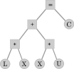
Figure 3: Tree representation of the equation $LX+XU=C$.

The algorithm starts by visiting the node corresponding to the operand $L$. There it establishes that, since $L$ is lower triangular, the identity and the $2\times 2$ partitioning rules are the only admissible ones. Thus, the rows and the columns of $L$ are bound together, and the list becomes $\left[\;\{L_{r},L_{c}\},\{U_{r}\},\{U_{c}\},\{C_{r}\},\{C_{c}\},\right.$ $\left.\{X_{r}\},\{X_{c}\}\;\right].$ The next node to be visited is that of the operand $X$. Since $X$ has no specific structure, its analysis causes no bindings. Then, the node corresponding to the $\ast$ operator is analyzed. The dimensions of $L$ and $X$ have to agree according to the matrix product, therefore, a binding between $L_{c}$ and $X_{r}$ is imposed: $\left[\;\{L_{r},L_{c},X_{r}\},\{U_{r}\},\{U_{c}\},\{C_{r}\},\{C_{c}\},\{X_{c}\}\;\right].$ At this stage the dimensions of the product $LX$ are also determined to be $L_{r}\times X_{c}$.

The procedure continues by analyzing the subtree corresponding to the product $XU$. Again, the lack of a specific structure in $X$ does not cause any binding and the algorithm follows with the study of the node for the operand $U$. The triangularity of $U$ imposes a binding between $U_{r}$ and $U_{c}$ leading to $\left[\;\{L_{r},L_{c},X_{r}\},\{U_{r},U_{c}\},\{C_{r}\},\{C_{c}\},\{X_{c}\}\;\right].$ Then, the node for the $\ast$ operator is analyzed, and a binding between $X_{c}$ and $U_{r}$ is found: $\left[\;\{L_{r},L_{c},X_{r}\},\{U_{r},U_{c},X_{c}\},\right.$ $\left.\{C_{r}\},\{C_{c}\}\;\right].$ The dimensions of the product $XU$ are determined to be $X_{r}\times U_{c}$.

The next node to be considered is the corresponding to the $+$ operator. It imposes a binding between the rows and the columns of the products $LX$ and $XU$, i.e., between $L_{r}$ and $X_{r}$, and between $X_{c}$ and $U_{c}$. Since each of these pairs of dimensions already belong to the same set, no modifications are made to the list. The algorithm establishes that the dimensions of the $+$ node are $L_{r}\times U_{c}$. Next, the node associated to the operand $C$ is analyzed. Since $C$ has no particular structure, its analysis does not cause any modification. The last node to be processed is the equality operator $=$. This node binds the rows of $C$ to those of $L$ ($C_{r}$, $L_{r}$) and the columns of $C$ to those of $U$ ($C_{c}$, $U_{c}$). The final list consists of two separate groups of dimensions:

$$\left[\;\{L_{r},L_{c},X_{r},C_{r}\},\{U_{r},U_{c},X_{c},C_{c}\}\;\right].$$

Having created $g$ groups of bound dimensions, the algorithm generates $2^{g}$ combinations of rules (the dimensions within each group being either partitioned or not), resulting in a family of partioned postconditions, one per combination. In practice, since the combination including solely identity rules does not lead to a PME, only $2^{g}-1$ combinations are acceptable. In our example the algorithm found two groups of bound dimensions, therefore three possible combinations of rules are generated: 1) only the dimensions in the second group are partitioned, 2) only the dimensions in the first group are partitioned, or 3) all dimensions are partitioned. The resulting partitionings are listed in Tab. 2.

#	L	U	C	X
1	$(L)$	$\left(\begin{array}[]{@{}c@{\,}|@{\,}c@{}}U_{TL}&U_{TR}\\ \hline\cr 0&U_{BR}\end{array}\right)$	$\left(\begin{array}[]{@{}c@{\,}|@{\,}c@{}}C_{L}&C_{R}\end{array}\right)$	$\left(\begin{array}[]{@{}c@{\,}|@{\,}c@{}}X_{L}&X_{R}\end{array}\right)$
2	$\left(\begin{array}[]{@{}c@{\,}|@{\,}c@{}}L_{TL}&0\\ \hline\cr L_{BL}&L_{BR}\end{array}\right)$	$(U)$	$\left(\begin{array}[]{@{}c@{}}C_{T}\\ \hline\cr C_{B}\end{array}\right)$	$\left(\begin{array}[]{@{}c@{}}X_{T}\\ \hline\cr X_{B}\end{array}\right)$
3	$\left(\begin{array}[]{@{}c@{\,}|@{\,}c@{}}L_{TL}&0\\ \hline\cr L_{BL}&L_{BR}\end{array}\right)$	$\left(\begin{array}[]{@{}c@{\,}|@{\,}c@{}}U_{TL}&U_{TR}\\ \hline\cr 0&U_{BR}\end{array}\right)$	$\left(\begin{array}[]{@{}c@{\,}|@{\,}c@{}}C_{TL}&C_{TR}\\ \hline\cr C_{BL}&C_{BR}\end{array}\right)$	$\left(\begin{array}[]{@{}c@{\,}|@{\,}c@{}}X_{TL}&X_{TR}\\ \hline\cr X_{BL}&X_{BR}\end{array}\right)$

Table 2: Viable combinations of partitioning rules for the Sylvester equation.

This very same process is used to find the bound dimensions of every target operation and, accordingly, only each and every viable combination of partitioning rules is generated.

4 Matrix Arithmetic and Pattern Matching

This section covers the second and third steps in the PME generation stage (Fig. 2). Within the Matrix Arithmetic step, symbolic arithmetic is performed and the = operator is distributed over the partitions, originating multiple equations. In (10) we display the result of these actions for the Cholesky factorization, where the symbol $\star$ means that the equation in the top-right quadrant is the transpose of the bottom-left one.

$$\left(\begin{array}[]{@{}c@{\,}|@{\,}c@{}}L_{TL}&0\\ \hline\cr L_{BL}&L_{BR}\end{array}\right)\!\!\left(\begin{array}[]{@{}c@{\,}|@{\,}c@{}}L_{TL}^{T}&L_{BL}^{T}\\ \hline\cr 0&L_{BR}^{T}\end{array}\right)\!=\!\left(\begin{array}[]{@{}c@{\,}|@{\,}c@{}}A_{TL}&A_{BL}^{T}\\ \hline\cr A_{BL}&A_{BR}\end{array}\right)\Rightarrow\left(\begin{array}[]{@{}c@{\,}|@{\,}c@{}}L_{TL}L_{TL}^{T}=A_{TL}&\star\\ \hline\cr L_{BL}L_{TL}^{T}=A_{BL}&L_{BL}L_{BL}^{T}+L_{BR}L_{BR}^{T}=A_{BR}\end{array}\right).$$ (10)

The Pattern Matching step delivers the sought-after PME. Success of this process is dependent on the ability to identify expressions with known structure and properties. In order to facilitate pattern matching, we force equations to be in their canonical form. We state that an equation is in canonical form if a) its left-hand side only consists of those terms that contain at least one unknown object, and b) its right-hand side only consists of those terms that solely contain known objects.

This last step carries out an iterative process comprising three separate actions: 1) structural pattern matching: equations are matched against known patterns; 2) once a known pattern is matched, the unknown operands are flagged as known and the equation becomes a tautology; 3) algebraic manipulation: the remaining equations are rearranged in canonical form. We clarify the iterative process by illustrating, action by action, how Cl1ck works through the Cholesky factorization. The first iteration is depicted in Box 6, in which the top-left formula displays the initial state. In all the next expressions, green and red are used to highlight the known and unknown operands, respectively.

Structural pattern matching:

All the equations in Box 6LABEL:sub@sbox:it1a are in canonical form. Through pattern matching, the top-left quadrant is the only one for which a match is found. Cl1ck identifies the equation as a Cholesky factorization (Box 6LABEL:sub@sbox:it1b), since the pattern in Box 2 is satisfied: the system recognizes that i) $L_{TL}$ is lower triangular; ii) $A_{TL}$ is SPD; and iii) the structure of the equation matches the one in the postcondition ($LL^{T}=A$).

Exposing new available operands:

Having matched the top-left equation, Cl1ck turns the unknown operand $L_{TL}$ into $L_{TL}$, and propagates the information to all the other quadrants (Box 6LABEL:sub@sbox:it1c). As a result, the top-left equation becomes a tautology.

Algebraic manipulation:

All the remaining equations are still in canonical form, thus no operation takes place (Box 6LABEL:sub@sbox:it1d).

$\left(\begin{array}[]{c|c}{\color[rgb]{1.0,0.0,0.0}L_{TL}}{\color[rgb]{1.0,0.0,0.0}L_{TL}^{T}}={\color[rgb]{0,0.390625,0}A_{TL}}&\star\\ \hline\cr{\color[rgb]{1.0,0.0,0.0}L_{BL}}{\color[rgb]{1.0,0.0,0.0}L_{TL}^{T}}={\color[rgb]{0,0.390625,0}A_{BL}}&{\color[rgb]{1.0,0.0,0.0}L_{BL}}{\color[rgb]{1.0,0.0,0.0}L_{BL}^{T}}+{\color[rgb]{1.0,0.0,0.0}L_{BR}}{\color[rgb]{1.0,0.0,0.0}L_{BR}^{T}}={\color[rgb]{0,0.390625,0}A_{BR}}\end{array}\right)$

(a) Initial state.

$\left(\begin{array}[]{c|c}{\color[rgb]{1.0,0.0,0.0}\boxed{\!\!{L_{TL}}\!\!}}=\Gamma({\color[rgb]{0,0.390625,0}A_{TL}})&\star\\ \hline\cr{\color[rgb]{1.0,0.0,0.0}L_{BL}}{\color[rgb]{1.0,0.0,0.0}L_{TL}^{T}}={\color[rgb]{0,0.390625,0}A_{BL}}&{\color[rgb]{1.0,0.0,0.0}L_{BL}}{\color[rgb]{1.0,0.0,0.0}L_{BL}^{T}}+{\color[rgb]{1.0,0.0,0.0}L_{BR}}{\color[rgb]{1.0,0.0,0.0}L_{BR}^{T}}={\color[rgb]{0,0.390625,0}A_{BR}}\end{array}\right)$

(b) Top-left equation is identified as a Cholesky sub-problem.

$\left(\begin{array}[]{c|c}{\color[rgb]{0,0.390625,0}\boxed{\!\!{L_{TL}}\!\!}}=\Gamma({\color[rgb]{0,0.390625,0}A_{TL}})&\star\\ \hline\cr{\color[rgb]{1.0,0.0,0.0}L_{BL}}{\color[rgb]{0,0.390625,0}\boxed{\!\!{L_{TL}^{T}}\!\!}}={\color[rgb]{0,0.390625,0}A_{BL}}&{\color[rgb]{1.0,0.0,0.0}L_{BL}}{\color[rgb]{1.0,0.0,0.0}L_{BL}^{T}}+{\color[rgb]{1.0,0.0,0.0}L_{BR}}{\color[rgb]{1.0,0.0,0.0}L_{BR}^{T}}={\color[rgb]{0,0.390625,0}A_{BR}}\end{array}\right)$

(c) $L_{TL}$ becomes a known operand for the rest of equations.

$\left(\begin{array}[]{c|c}{\color[rgb]{0,0.390625,0}L_{TL}}=\Gamma({\color[rgb]{0,0.390625,0}A_{TL}})&\star\\ \hline\cr{\color[rgb]{1.0,0.0,0.0}L_{BL}}{\color[rgb]{0,0.390625,0}L_{TL}^{T}}={\color[rgb]{0,0.390625,0}A_{BL}}&{\color[rgb]{1.0,0.0,0.0}L_{BL}}{\color[rgb]{1.0,0.0,0.0}L_{BL}^{T}}+{\color[rgb]{1.0,0.0,0.0}L_{BR}}{\color[rgb]{1.0,0.0,0.0}L_{BR}^{T}}={\color[rgb]{0,0.390625,0}A_{BR}}\end{array}\right)$

(d) There is no need for algebraic manipulation.

Box 6 First iteration towards the PME generation.

In this first iteration, one unknown operand, $L_{TL}$, has become known, and one equation has turned into a tautology. The knowledge encoded in such a tautology is of importance for a subsequent iteration. The second iteration is shown in Box 7.

Structural pattern matching:

Box 7LABEL:sub@sbox:it2a reproduces the final state from the previous iteration. Among the two outstanding equations, the bottom-left one is identified (Box 7LABEL:sub@sbox:it2b), as it matches the pattern of a triangular system of equations with multiple right-hand sides (trsm). The pattern for a trsm is

$$\{XL^{T}=B\;\wedge\;{\tt{Output(}}X{\tt{)}}\;\wedge\;{\tt{Input(}}L{\tt{)}}\;\wedge\;{\tt{LowerTriangular(}}L{\tt{)}}\;\wedge\;{\tt{Input(}}B{\tt{)}}\}.$$

For the sake of brevity, we assume that Cl1ck had learned such pattern from a previous derivation; in practice, in case the system does not know the pattern, a nested task of PME generation would be initiated, yielding the required pattern.

Exposing new available operands:

Once the trsm is identified, the output operand $L_{BL}$ becomes available and turns to green in the bottom-right quadrant (Box 7LABEL:sub@sbox:it2c).

Algebraic manipulation:

The bottom-right equation is not in canonical form anymore: the product $L_{BL}L_{BL}^{T}$, now a known quantity, does not lay in the right-hand side. A simple manipulation brings the equation back to canonical form (Box 7LABEL:sub@sbox:it2d).

$\left(\begin{array}[]{c|c}{\color[rgb]{0,0.390625,0}L_{TL}}=\Gamma({\color[rgb]{0,0.390625,0}A_{TL}})&\star\\ \hline\cr{\color[rgb]{1.0,0.0,0.0}L_{BL}}{\color[rgb]{0,0.390625,0}L_{TL}^{T}}={\color[rgb]{0,0.390625,0}A_{BL}}&{\color[rgb]{1.0,0.0,0.0}L_{BL}}{\color[rgb]{1.0,0.0,0.0}L_{BL}^{T}}+{\color[rgb]{1.0,0.0,0.0}L_{BR}}{\color[rgb]{1.0,0.0,0.0}L_{BR}^{T}}={\color[rgb]{0,0.390625,0}A_{BR}}\end{array}\right)$

(a) Initial state.

$\left(\begin{array}[]{c|c}{\color[rgb]{0,0.390625,0}L_{TL}}=\Gamma({\color[rgb]{0,0.390625,0}A_{TL}})&\star\\ \hline\cr{\color[rgb]{1.0,0.0,0.0}\boxed{\!\!{L_{BL}}\!\!}}={\color[rgb]{0,0.390625,0}A_{BL}}{\color[rgb]{0,0.390625,0}L_{TL}^{-T}}&{\color[rgb]{1.0,0.0,0.0}L_{BL}}{\color[rgb]{1.0,0.0,0.0}L_{BL}^{T}}+{\color[rgb]{1.0,0.0,0.0}L_{BR}}{\color[rgb]{1.0,0.0,0.0}L_{BR}^{T}}={\color[rgb]{0,0.390625,0}A_{BR}}\end{array}\right)$

(b) Bottom-left equation is identified as a triangular system of equations.

$\left(\begin{array}[]{@{}c@{\,}|@{\,}c@{}}{\color[rgb]{0,0.390625,0}L_{TL}}=\Gamma({\color[rgb]{0,0.390625,0}A_{TL}})&\star\\ \hline\cr{\color[rgb]{0,0.390625,0}\boxed{\!\!{L_{BL}}\!\!}}={\color[rgb]{0,0.390625,0}A_{BL}}{\color[rgb]{0,0.390625,0}L_{TL}^{-T}}&{\color[rgb]{0,0.390625,0}\boxed{\!\!{L_{BL}^{\phantom{T}}}\!\!}}{\color[rgb]{0,0.390625,0}\boxed{\!\!{L_{BL}^{T}}\!\!}}+{\color[rgb]{1.0,0.0,0.0}L_{BR}}{\color[rgb]{1.0,0.0,0.0}L_{BR}^{T}}={\color[rgb]{0,0.390625,0}A_{BR}}\end{array}\right)$

(c) $L_{BL}$ becomes a known operand.

$\left(\begin{array}[]{c|c}{\color[rgb]{0,0.390625,0}L_{TL}}=\Gamma({\color[rgb]{0,0.390625,0}A_{TL}})&\star\\ \hline\cr{\color[rgb]{0,0.390625,0}L_{BL}}={\color[rgb]{0,0.390625,0}A_{BL}}{\color[rgb]{0,0.390625,0}L_{TL}^{-T}}&{\color[rgb]{1.0,0.0,0.0}L_{BR}}{\color[rgb]{1.0,0.0,0.0}L_{BR}^{T}}={\color[rgb]{0,0.390625,0}A_{BR}}-{\color[rgb]{0,0.390625,0}L_{BL}}{\color[rgb]{0,0.390625,0}L_{BL}^{T}}\end{array}\right)$

(d) State after the algebraic manipulation.

Box 7 Second iteration towards the PME generation.

The process continues until all the equations are turned into tautologies. The third and final iteration for the Cholesky factorization is shown in Box 8, where the top formula replicates the final state from the previous iteration.

Structural pattern matching:

Only one equation, the bottom-right one, remains unprocessed. At a first glance, one might recognize a Cholesky factorization, but the corresponding pattern in Box 2 requires $A$ to be SPD. The question is whether the expression $A_{BR}-L_{BL}L_{BL}^{T}$ represents an SPD matrix. In order to answer the question, Cl1ck applies rewrite rules and symbolic simplifications.

In Sect. 3.2 we explained that the following quantities are known to be SPD: $A_{TL}$, $A_{BR}$, $A_{TL}-A_{BL}^{T}A_{BR}^{-1}A_{BL}$, and $A_{BR}-A_{BL}A_{TL}^{-1}A_{BL}^{T}$. In order to determine whether $A_{BR}-L_{BL}L_{BL}^{T}$ is equivalent to any of these expressions, Cl1ck makes use of the knowledge acquired throughout the previous iterations. Specifically, in the first two iterations it was discovered that $L_{TL}L_{TL}^{T}=A_{TL}$, and $L_{BL}=A_{BL}L_{TL}^{-T}$. Using these tautologies as rewrite rules, the expression $A_{BR}-L_{BL}L_{BL}^{T}$ is manipulated. First, the equality $L_{BL}=A_{BL}L_{TL}^{-T}$ is used to replace the instances of $L_{BL}$, yielding $A_{BR}-A_{BL}L_{TL}^{-T}L_{TL}^{-1}A_{BL}^{T}$, and equivalently, $A_{BR}-A_{BL}(L_{TL}L_{TL}^{T})^{-1}A_{BL}^{T}$. Then, by virtue of the tautology $L_{TL}L_{TL}^{T}=A_{TL}$, $L_{TL}L_{TL}^{T}$ is replaced by $A_{TL}$, yielding $A_{BR}-A_{BL}A_{TL}^{-1}A_{BL}^{T}$. Now, this expression is known to be SPD. Thanks to these manipulations, Cl1ck successfully associates the bottom right equation with the pattern for a Cholesky factorization.

Exposing new available operands:

Once the expression in the bottom-right quadrant is identified, the system exposes the quantity $L_{BR}$ as known. Since no equation is left, the process completes and the PME—formed by the three tautologies—is returned as output.

$\left(\begin{array}[]{c|c}{\color[rgb]{0,0.390625,0}L_{TL}}=\Gamma({\color[rgb]{0,0.390625,0}A_{TL}})&\star\\ \hline\cr{\color[rgb]{0,0.390625,0}L_{BL}}={\color[rgb]{0,0.390625,0}A_{BL}}{\color[rgb]{0,0.390625,0}L_{TL}^{-T}}&{\color[rgb]{1.0,0.0,0.0}L_{BR}}{\color[rgb]{1.0,0.0,0.0}L_{BR}^{T}}={\color[rgb]{0,0.390625,0}A_{BR}}-{\color[rgb]{0,0.390625,0}L_{BL}}{\color[rgb]{0,0.390625,0}L_{BL}^{T}}\end{array}\right)$

(a) Initial state.

$\left(\begin{array}[]{c|c}{\color[rgb]{0,0.390625,0}L_{TL}}=\Gamma({\color[rgb]{0,0.390625,0}A_{TL}})&\star\\ \hline\cr{\color[rgb]{0,0.390625,0}L_{BL}}={\color[rgb]{0,0.390625,0}A_{BL}}{\color[rgb]{0,0.390625,0}L_{TL}^{-T}}&{\color[rgb]{1.0,0.0,0.0}\boxed{\!\!{L_{BR}}\!\!}}=\Gamma({\color[rgb]{0,0.390625,0}A_{BR}}-{\color[rgb]{0,0.390625,0}L_{BL}}{\color[rgb]{0,0.390625,0}L_{BL}^{T}})\end{array}\right)$

(b) Bottom-right equation is identified as a Cholesky factorization.

$\left(\begin{array}[]{c|c}{\color[rgb]{0,0.390625,0}L_{TL}}=\Gamma({\color[rgb]{0,0.390625,0}A_{TL}})&\star\\ \hline\cr{\color[rgb]{0,0.390625,0}L_{BL}}={\color[rgb]{0,0.390625,0}A_{BL}}{\color[rgb]{0,0.390625,0}L_{TL}^{-T}}&{\color[rgb]{0,0.390625,0}\boxed{\!\!{L_{BR}}\!\!}}=\Gamma({\color[rgb]{0,0.390625,0}A_{BR}}-{\color[rgb]{0,0.390625,0}L_{BL}}{\color[rgb]{0,0.390625,0}L_{BL}^{T}})\end{array}\right)$

(c) $L_{BR}$ becomes a known operand.

$\left(\begin{array}[]{c|c}{\color[rgb]{0,0.390625,0}L_{TL}}=\Gamma({\color[rgb]{0,0.390625,0}A_{TL}})&\star\\ \hline\cr{\color[rgb]{0,0.390625,0}L_{BL}}={\color[rgb]{0,0.390625,0}A_{BL}}{\color[rgb]{0,0.390625,0}L_{TL}^{-T}}&{\color[rgb]{0,0.390625,0}L_{BR}}=\Gamma({\color[rgb]{0,0.390625,0}A_{BR}}-{\color[rgb]{0,0.390625,0}L_{BL}}{\color[rgb]{0,0.390625,0}L_{BL}^{T}})\end{array}\right)$

(d) Final PME.

Box 8 Final iteration towards the PME generation.

By means of the described process, PMEs for a target equation are automatically generated. The PME for the Cholesky factorization is given in Box 9.

$$\left({\begin{array}[]{@{\,}c@{\,}|@{\,}c@{\,}}L_{TL}=\Gamma(A_{TL})&\star\\ \hline\cr L_{BL}=A_{BL}L_{TL}^{-T}&L_{BR}=\Gamma(A_{BR}-L_{BL}L_{BL}^{T})\end{array}}\right)$$

Box 9 Partitioned Matrix Expression for the Cholesky factorization.

5 Conclusions

The work we presented sets the ground for the development of a symbolic system that, from the sole description of an operation, generates algorithms automatically. The core of our methodology stands in the PME. A PME encapsulates the information about the target operation in a way that facilitates the subsequent identification of loop-invariants. The loop-invariants then lead to the final algorithms through a technique based on program correctness. In this paper we introduce a symbolic system, Cl1ck, that automates the generation of PMEs.

In order to generate PMEs, Cl1ck first identifies how the operands in the operation may be partitioned. Instead of a brute force approach of exponential complexity, Cl1ck utilizes a tree-based algorithm that yields only the viable sets of partitioning rules. Through a process of pattern matching, each such set leads to a distinct PME. The key in the PME generation is Cl1ck’s ability to identify known patterns. Initially, Cl1ck only recognizes elementary structures, but its knowledge expands by automatically learning the patterns associated with the operations it tackles. Thanks to this augmenting internal knowledge, the system may generate PMEs for increasingly complex operations.

To illustrate Cl1ck, we discussed the Cholesky factorization and, partially (due to space constraints), the Sylvester equation. Despite the fact that such operations differ in multiple ways—number and properties of the operands, number of valid sets of partitioning rules, number of PMEs—the steps performed by Cl1ck leading to the PMEs are exactly the same. As future work, we plan to add support for higher dimensional objects and the derivative operator.

6 Acknowledgements

The authors gratefully acknowledge the support received from the Deutsche Forschungsgemeinschaft (German Research Association) through grant GSC 111.

References

-
[1]
FLAME Project:
FLAME Online Reference.
http://z.cs.utexas.edu/wiki/flame.wiki/ - [2] Dongarra, J.J., Du Croz, J., Hammarling, S., Duff, I.S.: A set of level 3 basic linear algebra subprograms. ACM Trans. Math. Softw. 16 (March 1990) 1–17
- [3] Jonsson, I., Kågström, B.: Recursive blocked algorithms for solving triangular systems—part i: one-sided and coupled sylvester-type matrix equations. ACM Transactions on Mathematical Software 28(4) (2002) 392–415
- [4] Jonsson, I., Kågström, B.: Recursive blocked algorithms for solving triangular systems—part ii: Two-sided and generalized sylvester and lyapunov matrix equations. ACM Transactions on Mathematical Software 28(4) (2002) 416–435
- [5] Anderson, E., Bai, Z., Bischof, C., Blackford, S., Demmel, J., Dongarra, J., Du Croz, J., Greenbaum, A., Hammarling, S., McKenney, A., Sorensen, D.: LAPACK Users’ Guide. Third edn. Society for Industrial and Applied Mathematics, Philadelphia, PA (1999)
- [6] Whaley, R.C., Dongarra, J.: Automatically tuned linear algebra software. In: SuperComputing 1998: High Performance Networking and Computing. (1998)
- [7] Frigo, M., Johnson, S.G.: The design and implementation of FFTW3. Proceedings of the IEEE 93(2) (2005) 216–231 Special issue on “Program Generation, Optimization, and Platform Adaptation”.
- [8] Püschel, M., Moura, J.M.F., Johnson, J., Padua, D., Veloso, M., Singer, B., Xiong, J., Franchetti, F., Gacic, A., Voronenko, Y., Chen, K., Johnson, R.W., Rizzolo, N.: SPIRAL: Code generation for DSP transforms. Proceedings of the IEEE, special issue on “Program Generation, Optimization, and Adaptation” 93(2) (2005) 232– 275
- [9] Bientinesi, P., Gunnels, J.A., Myers, M.E., Quintana-Ortí, E.S., van de Geijn, R.A.: The science of deriving dense linear algebra algorithms. ACM Transactions on Mathematical Software 31(1) (March 2005) 1–26
- [10] Bientinesi, P., Quintana-Ortí, E.S., van de Geijn, R.: FLAMElab: A farewell to indices. FLAME Working Note #11. Technical Report TR-2003-11, The University of Texas at Austin, Department of Computer Sciences (April 2003)
- [11] Quintana-Ortí, E.S., van de Geijn, R.A.: Formal derivation of algorithms: The triangular Sylvester equation. ACM Transactions on Mathematical Software 29(2) (June 2003) 218–243
- [12] Poulson, J., van de Geijn, R., Bennighof, J.: Parallel algorithms for reducing the generalized hermitian-definite eigenvalue problem. FLAME Working Note #56. Technical Report TR-11-05, The University of Texas at Austin, Department of Computer Sciences (February 2011)
- [13] Bientinesi, P., van de Geijn, R.: A goal-oriented and modular approach to stability analysis. SIAM Journal on Matrix Analysis and Applications (2011) “To appear”.
-
[14]
Wolfram Research:
Mathematica Reference Guide.
http://reference.wolfram.com/mathematica/ - [15] Gries, D., Schneider, F.B.: A Logical Approach to Discrete Math. Texts and Monographs in Computer Science. Springer Verlag (1992)