Automatic Generation of Loop-Invariants
for Matrix Operations

Abstract

In recent years it has been shown that for many linear algebra operations it is possible to create families of algorithms following a very systematic procedure. We do not refer to the fine tuning of a known algorithm, but to a methodology for the actual generation of both algorithms and routines to solve a given target matrix equation. Although systematic, the methodology relies on complex algebraic manipulations and non-obvious pattern matching, making the procedure challenging to be performed by hand; our goal is the development of a fully automated system that from the sole description of a target equation creates multiple algorithms and routines. We present Cl1ck, a symbolic system written in Mathematica, that starts with an equation, decomposes it into multiple equations, and returns a set of loop-invariants for the algorithms—yet to be generated—that will solve the equation. In a successive step each loop-invariant is then mapped to its corresponding algorithm and routine. For a large class of equations, the methodology generates known algorithms as well as many previously unknown ones. Most interestingly, the methodology unifies algorithms traditionally developed in isolation. As an example, the five well known algorithms for the $LU$ factorization are for the first time unified under a common root.

I Introduction

In order to attain high-performance on a variety of architectures and programming paradigms, for a target operation not one but multiple algorithms are needed. We focus our attention on the domain of matrix equations and aim for a symbolic system, fully automated, that takes as input the description of an equation $Eq$ and returns algorithms and routines to solve $Eq$.

$$\left(\begin{array}[]{@{\,}c@{\,}}\{X_{T},Y_{T}\}=\Psi(A_{TL},B,C_{T},D_{TL},E,F_{T})\\ \hline\cr\{X_{B},Y_{B}\}=\Psi(A_{BR},B,C_{B}-A_{BL}X_{T},D_{BR},E,F_{B}-D_{BL}X_{T})\end{array}\right)$$

Box 1 Partitioned Matrix Expression for the coupled Sylvester equation.

This research is inspired by an existing methodology for the derivation of families of algorithms, which is based on formal methods and program correctness  [2, 3]. As depicted in Fig. 1, in the process of algorithm generation we identify three successive stages: “PME Generation”, “Loop-Invariant Identification”, and “Algorithm Derivation”. The input to the process is the description of a target operation. In the first stage, the Partitioned Matrix Expression (PME) for the operation is obtained. A PME is a decomposition of the original problem into simpler sub-problems in a “divide and conquer” fashion, exposing the computation to be performed in each part of the output matrices. As an example, in Box 1 we show the PME for the coupled Sylvester equation:

$$\begin{array}[]{c@{\quad\!}c@{\quad\!}c}\begin{aligned} \{X,Y\}=\Psi(&A,B,C,\\ &D,E,F)\end{aligned}&\equiv&\left\{\begin{array}[]{@{}l@{}}AX+YB=C\\ DX+YE=F\end{array}\right.\end{array}$$

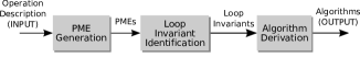
Figure 1: The process of algorithm generation can be broken down into three main stages.

The second stage of the process deals with the identification of boolean predicates, the Loop-Invariants [4], that describe the intermediate state of computation for the sought-after algorithms. Loop-invariants can be extracted from the PME, and are at the heart of the automation of the third stage. Box 2 contains an example of loop-invariant.

$$\left(\begin{array}[]{@{\,}c@{\,}}\{X_{T},Y_{T}\}=\Psi(A_{TL},B,C_{T},D_{TL},E,F_{T})\\ \hline\cr\neq\end{array}\right)$$

Box 2 One of the loop-invariants for the coupled Sylvester equation. The symbol $\neq$ indicates that no constraints on the contents of the variables are imposed.

In the third and last stage of the methodology, each loop-invariant is transformed into its corresponding loop-based algorithm. This stage makes use of classical concepts in computer science such as formal program correctness, Hoare’s triples, and the invariance theorem.

We consider this paper as the second in a series. In the first one [5] we introduced Cl1ck, a symbolic system written in Mathematica [6], for the automatic generation of algorithms. There we detailed how Cl1ck makes use of rewrite rules and pattern matching to automatically generate PMEs from the description of target operations. This paper centers around the second stage of the derivation process, the Loop-Invariant Identification. We describe the necessary steps to obtain a family of loop-invariants from a given PME, Fig. 2, and expose how Cl1ck automates them through an extensive usage of pattern matching and rewrite rules.

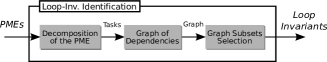
Figure 2: Steps for the identification of loop-invariants from a PME.

As in the example in Box 1, a PME decomposes the target operation into a set of equalities. Each of the equalities expresses the computation to be carried out in the different parts of the matrix to compute the overall equation. Since an equality may represent a complex operation, we first decompose it into a sequence of tasks. We define tasks as basic units of computation matched by simple patterns such as $C=A+B$, $C=AB$, $B=A^{-1}$ or $X=A^{-1}B$. Next, we inspect the tasks for dependencies among them, and build the corresponding dependency graph. Then, predicates that are candidates to becoming loop-invariants are identified as subsets of the graph satisfying the dependencies. Such subgraphs represent tasks included in the equalities and, therefore, are equivalent to choosing subsets of the computation included in the PME. In the final step, the candidate predicates are checked for feasibility and the resulting ones are labelled as viable loop-invariants.

The methodology described in [3] generates loop-based algorithms that all share a fixed structure: a basic initialization followed by a loop in which the actual computation is carried out (Box 3). The main idea of the methodology is to identify a loop-invariant on top of which a proof of correctness is built. Quoting Gries and Schneider from their book A Logical Approach to Discrete Math [4]

“Loop-invariants are crucial to understanding loops—so crucial that all but the most trivial loops should be documented with the invariants used to prove their annotations correct. In fact, (a first approximation to) the invariant should be developed before the loop is written and should act as a guide to the development of the loop.”

A loop-invariant has to be satisfied before the loop is entered and at the top and the bottom of each iteration. Upon completion of the loop, the loop-invariant as well as the negation of the loop-guard are satisfied. Given these known facts, the statements of the algorithms are chosen to satisfy them. In particular, the loop-invariant, $LI$, and the loop-guard, $G$, must be chosen so that $LI\wedge\neg G$ implies that the target equation has been solved.

$\{P_{\rm pre}\}$

Partition

$\{P_{\rm inv}\}$

While $G$ do

$\rm LoopBody$

end

$\{P_{\rm inv}\wedge\neg G\}$

$\{P_{\rm post}\}$

Box 3 Template for a formal proof of correctness for algorithms consisting of an initialization step followed by a loop.

As the complexity of the target equation increases, the methodology requires longer and more involved algebraic manipulation and pattern matching, making the manual generation of algorithms a tedious and error-prone process. The situation is aggravated by the fact that not one but multiple algorithms are desired for one same target equation. For this reason we advocate an automated symbolic system which exploits the capabilities of modern computer algebra tools to carry out the entire derivation process.

In this paper, we make progress towards such a vision detailing how Cl1ck performs all the steps involved in the Loop-Invariant Identification. The paper is organized as follows. In Section II we illustrate the formalism used to describe the target operations. The automatic generation of PMEs is reviewed in Section III. In Section IV we detail how loop-invariants are identified and how the process is automated, while in section V a more challenging example is treated. We draw conclusions in Section VI.

II Input to Cl1ck

In line with the methodology we follow for the derivation of algorithms, we choose the formalism traditionally used to reason about program correctness: operations shall be specified by means of the predicates Precondition ($P_{\rm pre}$) and Postcondition ($P_{\rm post}$) [4]. The precondition enumerates the operands that appear in the equation and describes their properties, while the postcondition specifies the equation that combines the operands.

As an example, Box 4 contains the description of the $LU$ factorization. The precondition states that the unit-diagonal, lower triangular matrix $L$ and the upper triangular matrix $U$ are unknown, and $A$ is an input matrix for which the $LU$ factorization exists. The postcondition indicates that, when the computation completes, the product $LU$ equals $A$; while the notation $\{L,U\}=LU(A)$ denotes that $L$ and $U$ are the $LU$ factors of $A$.

$$\{L,U\}=LU(A)\equiv\left\{\begin{split}P_{\rm pre}:\{&{\tt{Unknown(}}L{\tt{)}}\,\wedge\,{\tt{LowTri(}}L{\tt{)}}\,\wedge\\ &{\tt{UnitDiag(}}L{\tt{)}}\,\wedge\\ &{\tt{Unknown(}}U{\tt{)}}\,\wedge\,{\tt{UppTri(}}U{\tt{)}}\,\wedge\\ &{\tt{Known(}}A{\tt{)}}\,\wedge\,{\tt{\exists\;LU(}}A{\tt{)}}\}\\ \\ P_{\rm post}:\{&LU=A\}\end{split}\right.$$

Box 4 Formal description for the $LU$ factorization.

The two predicates in Box 4 describe unambiguously the $LU$ factorization and characterize the only knowledge about the operation needed by Cl1ck to automate the generation of algorithms. Box 5 illustrates the corresponding Mathematica statements required from the user.

precondition = {    { L, {"Output", "Matrix", "LowerTriangular",          "UnitDiagonal"} },    { U, {"Output", "Matrix", "UpperTriangular"} },    { A, {"Input",  "Matrix", "ExistsLU"} }};postcondition = {    { equal[times[L , U], A] } (* L U = A *)};

Box 5 Mathematica representation of the precondition and postcondition predicates for the $LU$ factorization.

We use the pair of predicates, $P_{\rm pre}$ and $P_{\rm post}$, to describe every target operation. Such a description is the input to the generation of PMEs and, therefore, to the whole process of algorithms derivation.

III Generation of PMEs

Having established a formalism to input a target operation, here we summarize the process of PME generation. Since the objective is a Partitioned Matrix Expression, Cl1ck starts off by rewriting the equation in the postcondition in terms of partitioned matrices. To this end, we introduce a set of rules to partition operands. As shown in Box 6, a generic matrix $A$ can be partitioned in four different ways. For a vector, only the $2\times 1$ and $1\times 1$ rules apply, while for scalars only the $1\times 1$ rule is admissible.

$\begin{aligned} A_{m\times n}\rightarrow&\left(\begin{array}[]{@{}c@{\,}|@{\,}c@{}}A_{TL}&A_{TR}\\ \hline\cr A_{BL}&A_{BR}\end{array}\right)\\ \small\textnormal{where }&A_{TL}\textnormal{ is }k_{1}\times k_{2}\end{aligned}$

(a) $2\times 2$ rule

$\begin{aligned} A_{m\times n}\rightarrow&\left(\begin{array}[]{@{}c@{}}A_{T}\\ \hline\cr A_{B}\end{array}\right)\\ \small\textnormal{where }&A_{T}\textnormal{ is }k_{1}\times n\end{aligned}$

(b) $2\times 1$ rule

$\begin{aligned} A_{m\times n}\rightarrow&\left(\begin{array}[]{@{}c@{\,}|@{\,}c@{}}A_{L}&A_{R}\end{array}\right)\\ \small\textnormal{where }&A_{L}\textnormal{ is }m\times k_{2}\end{aligned}$

(c) $1\times 2$ rule

$\begin{aligned} A_{m\times n}\rightarrow&\left(\begin{array}[]{@{}c@{}}A\end{array}\right)\\ \small\textnormal{where }&A\textnormal{ is }m\times n\end{aligned}$

(d) $1\times 1$ rule

Box 6 Rules for partitioning a generic matrix operand A. We use the subscript letters $T$, $B$, $L$, and $R$ for $T$op, $B$ottom, $L$eft, and $R$ight, respectively.

The partitionings for an operand are constrained not only by its type (matrix, vector or scalar) but also by its structure: if the operand presents a known structure, such as triangularity or symmetry, we restrict the viable partitionings to those that allow the inheritance of properties. For instance, Box 7 illustrates the admissible partitionings for a lower triangular matrix $L$. Only two rules allow the inheritance: when the $1\times 1$ rule is applied, $L$ remains unchanged, and therefore triangular; a constrained $2\times 2$ rule in which the $TL$ quadrant is square leads a partitioning where both $L_{TL}$ and $L_{BR}$ are square and lower triangular, $L_{TR}$ is zero, and $L_{BL}$ is a generic matrix.

$\begin{aligned} L_{m\times m}\rightarrow&\left(\begin{array}[]{@{}c@{\,}|@{\,}c@{}}L_{TL}&0\\ \hline\cr L_{BL}&L_{BR}\end{array}\right)\\ \small\textnormal{where }&L_{TL}\textnormal{ is }k\times k\end{aligned}$  or

$\begin{aligned} L_{m\times m}\rightarrow&\left(\begin{array}[]{@{}c@{}}L\end{array}\right)\\ \small\textnormal{where }&L\textnormal{ is }m\times m\end{aligned}$

Box 7 Partitioning rules for a lower triangular matrix $L$.

Finally, the viable partitionings are also constrained by the operators that appear in the postcondition. For instance, in the $LU$ factorization, the operator times in $LU$ imposes that if $L$ is partitioned along the columns, then $U$ has to be partitioned along the rows and vice versa, so that the product is well defined. Since the set of rules where all the operands are partitioned $1\times 1$ does not lead to a Partitioned Matrix Expression, the only admissible set of partitioning rules for the $LU$ factorization is shown in Box 8. An efficient algorithm that identifies all the admissible partitioning rules for a given equation was introduced in [5].

$$\begin{array}[]{c}\begin{aligned} L_{m\times m}\rightarrow&\left(\begin{array}[]{@{}c@{\,}|@{\,}c@{}}L_{TL}&0\\ \hline\cr L_{BL}&L_{BR}\end{array}\right)\\ \small\textnormal{where }&L_{TL}\textnormal{ is }k\times k\end{aligned}\raisebox{7.96677pt}{{, }}\hskip 14.22636pt\begin{aligned} U_{m\times m}\rightarrow&\left(\begin{array}[]{@{}c@{\,}|@{\,}c@{}}U_{TL}&U_{TR}\\ \hline\cr 0&U_{BR}\end{array}\right)\\ \small\textnormal{where }&U_{TL}\textnormal{ is }k\times k\end{aligned}\raisebox{6.82864pt}{{ and }}\\[28.45274pt] \begin{aligned} A_{m\times m}\rightarrow&\left(\begin{array}[]{@{}c@{\,}|@{\,}c@{}}A_{TL}&A_{TR}\\ \hline\cr A_{BL}&A_{BR}\end{array}\right)\\ \small\textnormal{where }&A_{TL}\textnormal{ is }k\times k\end{aligned}\end{array}$$

Box 8 Set of partitioning rules for the $LU$ factorization.

Once the valid partitioning rules are found, Cl1ck applies them to the postcondition to obtain a predicate called partitioned postcondition. In the case of the $LU$ factorization, the corresponding partitioned postcondition is

$$\begin{array}[]{l}LU=A\;\Rightarrow\;\left(\begin{array}[]{@{}c@{\,}|@{\,}c@{}}L_{TL}&0\\ \hline\cr L_{BL}&L_{BR}\end{array}\right)\left(\begin{array}[]{@{}c@{\,}|@{\,}c@{}}U_{TL}&U_{TR}\\ \hline\cr 0&U_{BR}\end{array}\right)=\left(\begin{array}[]{@{}c@{\,}|@{\,}c@{}}A_{TL}&A_{TR}\\ \hline\cr A_{BL}&A_{BR}\end{array}\right)\end{array}.$$

From here, matrix arithmetic is carried out until the equality operator is distributed over the partitions yielding a set of equalities, one per quadrant:

$$\left(\begin{array}[]{@{}c@{\,}|@{\,}c@{}}L_{TL}&0\\ \hline\cr L_{BL}&L_{BR}\end{array}\right)\left(\begin{array}[]{@{}c@{\,}|@{\,}c@{}}U_{TL}&U_{TR}\\ \hline\cr 0&U_{BR}\end{array}\right)=\left(\begin{array}[]{@{}c@{\,}|@{\,}c@{}}A_{TL}&A_{TR}\\ \hline\cr A_{BL}&A_{BR}\end{array}\right)\quad\Rightarrow$$ (7)

$$\left(\begin{array}[]{@{}c@{\,}|@{\,}c@{}}L_{TL}U_{TL}&L_{TL}U_{TR}\\ \hline\cr L_{BL}U_{TL}&L_{BL}U_{TR}+L_{BR}U_{BR}\end{array}\right)=\left(\begin{array}[]{@{}c@{\,}|@{\,}c@{}}A_{TL}&A_{TR}\\ \hline\cr A_{BL}&A_{BR}\end{array}\right)\quad\Rightarrow$$ (12)

$$\left(\begin{array}[]{@{}c@{\,}|@{\,}c@{}}L_{TL}U_{TL}=A_{TL}&L_{TL}U_{TR}=A_{TR}\\ \hline\cr L_{BL}U_{TL}=A_{BL}&L_{BL}U_{TR}+L_{BR}U_{BR}=A_{BR}\end{array}\right).$$ (15)

At this point, an iterative process involving algebraic manipulation and pattern matching transforms Eq. 7 into the sought-after PME. Central to this step is the capability of Cl1ck to learn the pattern that defines the target operation. Initially Cl1ck only knows the pattern for a set of basic operations: addition, multiplication, inversion and transposition. This information is hard-coded. More patterns are discovered while tackling new operations. For instance, the definition of the $LU$ factorization in Box 4 defines a pattern. The pattern establishes that two matrices $X$ and $Y$ are the $LU$ factors of a matrix $Z$ if the constraints in the precondition are satisfied, and $X$, $Y$ and $Z$ are related as dictated by the postcondition ($XY=Z$). Such patterns provide Cl1ck with the necessary knowledge to identify known operations within each of the equalities in Eq. 7.

Thanks to the inheritance of properties, the system recognizes that the matrices $L_{TL}$, $U_{TL}$ and $A_{TL}$ match the pattern in Box 4, and therefore asserts that $\{L_{TL},U_{TL}\}=LU(A_{TL})$. Similarly, Cl1ck identifies that $U_{TR}$ and $L_{BL}$ result from two triangular systems, and that $L_{BR}$ and $U_{BR}$ are the $LU$ factors of an updated matrix $A_{BR}$. Box 9 contains the outcome of this process, the PME for the $LU$ factorization. Notice that no restrictions on the size of the sub-operands was imposed; the decomposition expressed by the PME is valid independently of the size of the sub-operands, provided that $L_{TL}$, $U_{TL}$ and $A_{TL}$ are square.

$$\left({\begin{array}[]{@{\;}c@{\;}|@{\;}c@{\;}}\{L_{TL},U_{TL}\}=LU(A_{TL})&U_{TR}=L_{TL}^{-1}A_{TR}\\ \hline\cr L_{BL}=A_{BL}U_{TL}^{-1}&\{L_{BR},U_{BR}\}=LU(A_{BR}-L_{BL}U_{TR})\end{array}}\right)$$

Box 9 Partitioned Matrix Expression for the $LU$ factorization.

IV Identification of Loop-Invariants

Loop-invariants are the key predicates to prove the correctness of loop-based algorithms. A loop-invariant expresses the state of the variables as the computation unfolds. Since a PME encapsulates the computation to be performed to solve a target equation, our approach identifies loop-invariants as subsets of the operations included in the PME.

The Loop-Invariant Identification process consists on three steps: 1) Cl1ck inspects each of the equalities included in the PME and decomposes them into a sequence of tasks, i.e., basic units of computation; 2) an analysis of the tasks yields the dependencies among them, leading to a graph of dependencies where the nodes are the tasks and the edges are the dependencies; 3) Cl1ck traverses the graph selecting all possible subgraphs satisfying the dependencies. The subgraphs correspond to predicates that are candidates to becoming loop-invariants. Cl1ck checks the feasibility of such predicates, discarding the non-feasible ones and promoting the remaining ones to loop-invariants.

IV-A Decomposition of the PME

Cl1ck commences by analyzing the equalities in the PME. Each equality satisfies a canonical form where the left-hand side contains the output sub-operand(s) and the right-hand side the explicit computation to obtain the output quantity(ies). The right-hand side may be expressed either as a combination of sub-operands and the basic operators (plus, times, transpose, inverse) or as an explicit function with one or more input arguments. In this first step Cl1ck decomposes the right-hand side of each equality into a sequence of one or more tasks.

The decomposition is led by a set of rules based on pattern matching to identify whether an expression is a basic task or a complex computation. In the case of a complex computation, such rules also express how to decompose it into simpler expressions. In this and following sections we use the examples to illustrate the decomposition rules.

We start the discussion with the $LU$ factorization example. As Box 9 shows, its PME comprises four equalities. The decomposition of equalities can be performed independently from one another; Cl1ck arbitrarily traverses the equalities by rows. The analysis commences from the top-left quadrant: $\{L_{TL},U_{TL}\}=LU(A_{TL}).$ Since the right-hand side matches a pattern associated to a basic task $\tt{f(x_{0},x_{1},\ldots,x_{n})}\wedge\forall{x_{i}}\,|\tt{isSuboperandQ}(x_{i})$, a function where all the input arguments are (sub-)operands, no decomposition is necessary and the system only returns one task: $\{L_{TL},U_{TL}\}:=LU(A_{TL}).$

The analysis procedes with the top-right quadrant: $U_{TR}=L_{TL}^{-1}A_{TR}.$ The expression is matched by the pattern $\tt{X=A^{-1}B}\wedge\tt{isLowTriQ}(A)\wedge\tt{NonSingularQ}(A)$ and corresponds to the solution of a triangular system of equations. Cl1ck recognizes it as a basic task and returns it. Similarly for the bottom-left quadrant in which a third task is identified.

Only one equality remains to be studied: $\{L_{BR},U_{BR}\}=LU(A_{BR}-L_{BL}U_{TR})$. The expression matches the pattern $\tt{f(x_{0},x_{1},\ldots,x_{n})\wedge\exists{x_{i}}|\neg{\tt{isSuboperandQ}}(x_{i})}$, meaning that at least one of the input arguments is not a (sub-)operand. Each complex argument is, therefore, recursively analyzed to identify a sequence of basic tasks. In the example, $A_{BR}-L_{BL}U_{TR}$ is the only complex argument; it is matched by the pattern $\tt{A-BC}$, corresponding to a basic task. As a result, Cl1ck yields the list {$A_{BR}:=A_{BR}-L_{BL}U_{TR}$, $\{L_{BR},U_{BR}\}:=LU(A_{BR})$}. In total, the algorithm produces the following five tasks:

1. $\{L_{TL},U_{TL}\}:=LU(A_{TL});$
   

2. $U_{TR}:=L_{TL}^{-1}A_{TR};$
   

3. $L_{BL}:=A_{BL}U_{TL}^{-1};$
   

4. $A_{BR}:=A_{BR}-L_{BL}U_{TR};$
   

5. $\{L_{BR},U_{BR}\}:=LU(A_{BR}).$
   

IV-B Graph of dependencies

Once the decomposition into tasks is available, Cl1ck proceeds with the study of the dependencies among them. Three different kinds of dependencies may occur.

• True dependency. One of the input arguments of a task is also the result of a previous task:

  $$\begin{array}[]{@{}c@{\;}c@{\;}c@{}}A&:=&B+C\\ X&:=&A+D\end{array}$$

  The order of the updates cannot be reversed because the second one requires the value of $A$ computed in the first one.

• Anti dependency. One of the input arguments of a task is also the result of a subsequent task:

  $$\begin{array}[]{@{}c@{\;}c@{\;}c@{}}X:=A+D\\ A:=B+C\end{array}$$

  The order of the updates cannot be reversed because the first update needs the value of $A$ before the second one overwrites it.

• Output dependency. The result of a task is also the result of a different task:

  $$\begin{array}[]{@{}c@{\;}c@{\;}c@{}}A:=B+C\\ A:=D+E\end{array}$$

  The second update cannot be performed until the first is computed to ensure the correct final value of $A$.

At a first sight, in the context of PMEs, it is difficult to distinguish between true and anti dependencies since there is no clear order in the execution. However, since each equality refers to the computation of a different part of the output matrices, any time the output of an equality is found as an input argument of another one, it implies a true dependency: first the quantity is computed, then it is used in a different equality.

Also, for the same reason, it is not easy to distinguish the direction of an output dependency. Since output dependencies only occur among tasks belonging to the same equality (each equality writes to a different part of the output matrices), the order is determined because one of the involved tasks comes from the decomposition of the other one, imposing an order in their execution. While in general all three types of dependencies may appear, in the examples we provide only true dependencies arise.

We detail the analysis of the dependencies following the example of the $LU$ factorization. During the analysis we use boldface to highlight the dependencies. The study commences with Task 1, whose output is $\{L_{TL},U_{TL}\}$. Cl1ck finds that the sub-operands $L_{TL}$ and $U_{TL}$ are input arguments for Tasks 2 and 3, respectively.

1. $\mathbf{\{L_{TL},U_{TL}\}}:=LU(A_{TL})$
   

2. $U_{TR}:=\mathbf{L_{TL}}^{-1}A_{TR}$
   

3. $L_{BL}:=A_{BL}\mathbf{U_{TL}}^{-1}$
   

This means that two true dependencies exist: one from Task 1 to Task 2 and another from Task 1 to Task 3. Next, Cl1ck inspects Task 2, whose output is $U_{TR}$. $U_{TR}$ is also identified as input for Task 4.

1. $\mathbf{U_{TR}}:=L_{TL}^{-1}A_{TR}$
   

2. $A_{BR}:=A_{BR}-L_{BL}\mathbf{U_{TR}}$
   

Hence, a true dependency from Tasks 2 to 4 is imposed. A similar situation arises when inspecting Task 3, originating a true dependency from Task 3 to Task 4.

The analysis continues with Task 4; this computes an update of $A_{BR}$, which is then used as input by Task 5, thus, creating one more true dependency.

1. $\mathbf{A_{BR}}:=A_{BR}-L_{BL}U_{TR}$
   

2. $\{L_{BR},U_{BR}\}:=LU(\mathbf{A_{BR}})$
   

Task 5 remains to be analyzed. Since its output, $\{L_{BR},U_{BR}\}$, does not appear in any of the other tasks, no new dependencies are found.

In Fig. 3, the list of the dependencies for the $LU$ factorization are mapped onto the graph in which node $i$ represents Task $i$.

Figure 3: Final graph of dependencies for the $LU$ factorization.

IV-C DAG subsets selection

Once Cl1ck has generated the dependency graph it selects all the possible subgraphs that satisfy the dependencies. Each of the subgraphs corresponds to a different loop-invariant, provided that it is feasible. The algorithm starts by sorting the nodes in the dependency graph; as such a graph is a DAG (direct acyclic graph), the nodes may be sorted by levels according to the longest path from the root. For the $LU$ factorization the sorted DAG is shown in Fig. 4.

Figure 4: Result of sorting by levels the graph of dependencies for the $LU$ factorization.

Cl1ck creates the list of subgraphs of the DAG incrementally, by levels. At first it initializes the list of subgraphs with the empty subset, $l=[\{\}]$, which is equivalent to selecting none of the PME tasks. Then, at each level it extends the set of subgraphs by adding all those resulting from appending the accesible nodes to the existing ones. A node at a given level is accesible from a subgraph $g$ if all the dependencies of the node are satisfied by $g$. Fig. 5 includes a sketch of the algorithm.

In the first iteration of the $LU$ example, the only accesible node from $\{\}$ at level 1 is node 1, hence, union($\{\}$, $\{1\}$) is added to $l$ which becomes $[\{\},\{1\}]$. Now, the level is increased to 2; no node in level 2 is accesible from $\{\}$, while both nodes 2 and 3 are accesible from $\{1\}$. The union of $\{1\}$ with the non-empty subsets of $\{2,3\}$—$\{2\}$, $\{3\}$ and $\{2,3\}$—are added to $l$, resulting in $l=[\{\},\{1\},\{1,2\},\{1,3\},\{1,2,3\}]$. At level 3, Cl1ck discovers that node 4 is accesible from subgraph $\{1,2,3\}$, thus $\{1,2,3,4\}$ is added to $l$. Finally, node 5 is accesible from $\{1,2,3,4\}$. The final list of subgraphs is:

$$[\{\},\{1\},\{1,2\},\{1,3\},\{1,2,3\},\{1,2,3,4\},\{1,2,3,4,5\}].$$

The seven subgraphs included in the final list correspond to predicates that are candidates to becoming loop-invariants. To this end, Cl1ck checks each predicate to establish its feasibility. The methodology we follow imposes two constraints for such a predicate $P$ to be a feasible loop-invariant: 1) there must exist a basic initialization of the operands, i.e., an initial partitioning, that renders the predicate $P$ true; 2) $P$ and the negation of the loop-guard, $G$, must imply the postcondition, $P_{\rm post}$, of the target operation: $P\wedge\neg G\implies P_{\rm post}$.

Following these rules the predicates corresponding to the empty and the full subgraphs of the DAG are always discarded. The former because it is analogous to an empty predicate and no matter what $G$ is, the implication $P\wedge\neg G\implies P_{\rm post}$ is not satisfied; the latter because it corresponds to the complete computation of the operation and, therefore, no basic initialization can be found to render the predicate $P$ true.

Cl1ck reaches to the same conclusion by identifying the initial and final state of the partitionings of the operands and rewriting the predicates in terms of such partitionings. A detailed discussion through the $LU$ example follows.

Algorithm: Generation of the subgraphs of a DAG

⬇

l = [{}]

for each level i:

for each subgraph g in l:

acc = accesiblesNodesFrom(g, i)

sub = nonEmptySubsets(acc)

for each s in sub:

append(l, union(g, s))

end

end

Figure 5: Algorithm to obtain all the possible subgraphs of a DAG.

Initially Cl1ck determines the direction in which the operands are traversed. In the example, all the operands are visited from the top-left to the bottom-right corner. The resulting initial partitionings are shown in Box 10.

$$\begin{array}[]{c}\begin{aligned} L_{m\times m}\rightarrow&\left(\begin{array}[]{@{}c@{\,}|@{\,}c@{}}L_{TL}&0\\ \hline\cr L_{BL}&L_{BR}\end{array}\right)\\ \small\textnormal{where }&L_{TL}\textnormal{ is }0\times 0\end{aligned}\raisebox{7.96677pt}{{, }}\hskip 14.22636pt\begin{aligned} U_{m\times m}\rightarrow&\left(\begin{array}[]{@{}c@{\,}|@{\,}c@{}}U_{TL}&U_{TR}\\ \hline\cr 0&U_{BR}\end{array}\right)\\ \small\textnormal{where }&U_{TL}\textnormal{ is }0\times 0\end{aligned}\raisebox{6.82864pt}{{ and }}\\[28.45274pt] \begin{aligned} A_{m\times m}\rightarrow&\left(\begin{array}[]{@{}c@{\,}|@{\,}c@{}}A_{TL}&A_{TR}\\ \hline\cr A_{BL}&A_{BR}\end{array}\right)\\ \small\textnormal{where }&A_{TL}\textnormal{ is }0\times 0\end{aligned}\end{array}$$

Box 10 Initial partitioning of the operands for the $LU$ factorization.

This knowledge is enough to rule the subgraph $\{1,2,3,4,5\}$ out; the application of the rules in Box 10 to the associated predicate $P$

$$\begin{array}[]{c}\begin{aligned} L_{m\times m}\rightarrow&\left(\begin{array}[]{@{}c@{\,}|@{\,}c@{}}L_{TL}&0\\ \hline\cr L_{BL}&L_{BR}\end{array}\right)\\ \small\textnormal{where }&L_{TL}\textnormal{ is }m\times m\end{aligned}\raisebox{7.96677pt}{{, }}\hskip 14.22636pt\begin{aligned} U_{m\times m}\rightarrow&\left(\begin{array}[]{@{}c@{\,}|@{\,}c@{}}U_{TL}&U_{TR}\\ \hline\cr 0&U_{BR}\end{array}\right)\\ \small\textnormal{where }&U_{TL}\textnormal{ is }m\times m\end{aligned}\raisebox{6.82864pt}{{ and }}\\[28.45274pt] \begin{aligned} A_{m\times m}\rightarrow&\left(\begin{array}[]{@{}c@{\,}|@{\,}c@{}}A_{TL}&A_{TR}\\ \hline\cr A_{BL}&A_{BR}\end{array}\right)\\ \small\textnormal{where }&A_{TL}\textnormal{ is }m\times m\end{aligned}\end{array}$$

Box 11 State of the partitioning of the operands for the $LU$ factorization upon completion of the loop.

#	Subgraph	Loop-invariant
1		$\left(\begin{array}[]{@{\,}c@{\,}|@{\,}c@{\,}}\{L_{TL},U_{TL}\}=LU(A_{TL})&\qquad\,\neq\qquad\phantom{}\\ \hline\cr\neq&\neq\end{array}\right)$
2		$\left(\begin{array}[]{@{\,}c@{\,}|@{\,}c@{\,}}\{L_{TL},U_{TL}\}=LU(A_{TL})&U_{TR}=L_{TL}^{-1}A_{TR}\\ \hline\cr\neq&\neq\end{array}\right)$
3		$\left(\begin{array}[]{@{\,}c@{\,}|@{\,}c@{\,}}\{L_{TL},U_{TL}\}=LU(A_{TL})&\qquad\,\neq\qquad\phantom{}\\ \hline\cr L_{BL}=A_{BL}U_{TL}^{-1}&\neq\end{array}\right)$
4		$\left(\begin{array}[]{@{\,}c@{\,}|@{\,}c@{\,}}\{L_{TL},U_{TL}\}=LU(A_{TL})&U_{TR}=L_{TL}^{-1}A_{TR}\\ \hline\cr L_{BL}=A_{BL}U_{TL}^{-1}&\neq\end{array}\right)$
5		$\left(\begin{array}[]{@{\,}c@{\,}|@{\,}c@{\,}}\{L_{TL},U_{TL}\}=LU(A_{TL})&U_{TR}=L_{TL}^{-1}A_{TR}\\ \hline\cr L_{BL}=A_{BL}U_{TL}^{-1}&A_{BR}=A_{BR}-L_{BL}U_{TR}\end{array}\right)$

TABLE I: The five loop-invariants for the $LU$ factorization.

$$\left(\begin{array}[]{@{\,}c@{\,}|@{\,}c@{\,}}\{L_{TL},U_{TL}\}=LU(A_{TL})&U_{TR}=L_{TL}^{-1}A_{TR}\\ \hline\cr L_{BL}=A_{BL}U_{TL}^{-1}&\{L_{BR},U_{BR}\}=LU(A_{BR}-L_{BL}U_{TR})\end{array}\right)$$

lead to a situation in which all quadrants are empty except for the bottom-right, where the computation of the $LU$ factorization of $A_{BR}$ is needed to satisfy $P$.

The initial partitionings determine that the valid loop-guard for the algorithm is $G=size(A_{TL})<size(A)$: initially the quadrant $A_{TL}$ is of size $0\times 0$; and at each iteration its size grows until it reaches the same size of $A$. The loop-guard $G$ implies that when the loop completes $A_{TL}$, $L_{TL}$ and $U_{TL}$ are of the same size of $A$, $L$ and $U$. Cl1ck exploits this fact to determine the feasibility of a predicate $P$. It applies the rewrite rules in Box 11 to $P$ and compares the result to the equation in the postcondition. Since the result of applying such rules to the empty predicate

$$\left(\begin{array}[]{@{\,}c@{\,}|@{\,}c@{\,}}\qquad\,\neq\qquad\phantom{}&\qquad\,\neq\qquad\phantom{}\\ \hline\cr\neq&\neq\end{array}\right),$$

where $\neq$ states that no constraints have to be satisfied, does not equal the postcondition it is discarded.

The other five predicates satisfy both feasibility constraints and are promoted to valid loop-invariants for the $LU$ factorization (Tab. I). It is important to point out that the five loop-invariants that Cl1ck identifies have been well known for a long time and are commonly presented in linear algebra textbooks[7]. At the same time, no explanation relative to their cardinality is ever provided and, most importantly, they are presented as distinct entities without a common root. It is only our systematic methodology that unifies these five algorithms for the $LU$ factorization.

V A more complex example: the coupled Sylvester equation

As a last study case, we show an example where the complexity of the graph of dependencies and the number of loop-invariants are such that the automation becomes an indispensable tool. This is by no means the most complex example Cl1ck may handle, but a compromise between a relatively complex example and the space needed to demonstrate it. In Box 12, the coupled Sylvester equation is defined.

#	Partitioned Matrix Expression
1	$\left(\begin{array}[]{@{\,}c@{\;}|@{\;}c@{\,}}\{X_{L},Y_{L}\}=\Psi(A,B_{TL},C_{L},D,E_{TL},F_{L})&\{X_{R},Y_{R}\}=\Psi(A,B_{BR},C_{R}-Y_{L}B_{TR},D,E_{BR},F_{R}-Y_{L}E_{TR})\end{array}\right)$
2	$\left(\begin{array}[]{@{\,}c@{\,}}\{X_{T},Y_{T}\}=\Psi(A_{TL},B,C_{T},D_{TL},E,F_{T})\\ \hline\cr\{X_{B},Y_{B}\}=\Psi(A_{BR},B,C_{B}-A_{BL}X_{T},D_{BR},E,F_{B}-D_{BL}X_{T})\end{array}\right)$
3	$\left(\begin{array}[]{@{\,}c@{\;}|@{\;}c@{\,}}\{X_{TL},Y_{TL}\}=\Psi(A_{TL},B_{TL},C_{TL},D_{TL},E_{TL},F_{TL})&\begin{aligned} \{X_{TR},Y_{TR}\}=\Psi(&A_{TL},B_{BR},C_{TR}-Y_{TL}B_{TR},\\ &D_{TL},E_{BR},F_{TR}-Y_{TL}E_{TR})\end{aligned}\\ \hline\cr\begin{aligned} \{X_{BL},Y_{BL}\}=\Psi(&A_{BR},B_{TL},C_{BL}-A_{BL}X_{TL},\\ &D_{BR},E_{TL},F_{BL}-D_{BL}X_{TL})\end{aligned}&\begin{aligned} \{X_{BR},Y_{BR}\}=\Psi(&A_{BR},B_{BR},C_{BR}-A_{BL}X_{TR}-Y_{BL}B_{TR},\\ &D_{BR},E_{BR},F_{BR}-D_{BL}X_{TR}-Y_{BL}E_{TR})\end{aligned}\end{array}\right)$

TABLE II: The three Partitioned Matrix Expressions for the coupled Sylvester equation.

The description in Box 12 is the input for Cl1ck. The system finds three feasible sets of partitioning rules for the operation. For each of the sets, Cl1ck applies the rules to the equation in the postcondition obtaining a partitioned postcondition. Then, the partitioned operands are combined and the equality operator is distributed obtaining an expression with multiple equalities. Cl1ck takes such expressions and, through a process based on pattern matching and algebraic manipulation, obtains the corresponding PMEs. The three resulting PMEs are listed in Tab. II

$$\begin{aligned} \{X,Y\}=\Psi(&A,B,C,\\ &D,E,F)\end{aligned}\equiv\left\{\begin{aligned} P_{\rm pre}:\{&{\tt{Known(}}A{\tt{)}}\,\!\wedge\,\!{\tt{LowTri(}}A{\tt{)}}\,\wedge\\ &{\tt{Known(}}B{\tt{)}}\,\!\wedge\,\!{\tt{UppTri(}}B{\tt{)}}\,\wedge\\ &{\tt{Known(}}D{\tt{)}}\,\!\wedge\,\!{\tt{LowTri(}}D{\tt{)}}\,\wedge\\ &{\tt{Known(}}E{\tt{)}}\,\!\wedge\,\!{\tt{UppTri(}}E{\tt{)}}\,\wedge\\ &{\tt{Known(}}C{\tt{)}}\,\!\wedge{\tt{Known(}}F{\tt{)}}\,\wedge\\ &{\tt{Unknown(}}X{\tt{)}}\,\!\wedge{\tt{Unknown(}}Y{\tt{)}}\\ \\ P_{\rm post}:&\left\{\begin{array}[]{@{}l@{}}AX+YB=C\\ DX+YE=F\end{array}\right.\end{aligned}\right.$$

Box 12 Formal description of the coupled Sylvester equation.

We continue the example by selecting the PME in the third row of Tab. II and describing the steps performed by Cl1ck to obtain loop-invariants. First, the system traverses the PME, one quadrant at a time, to decompose the equalities into basic tasks. The analysis starts from the top-left equality; since the right-hand side consists of a function where all the input arguments are sub-operands, the system yields the entire expression as a basic task.

• $\{X_{TL},Y_{TL}\}:=\Psi(A_{TL},B_{TL},C_{TL},D_{TL},E_{TL},F_{TL})$.

Next, the top-right equality is inspected. In this case, two of the input arguments are not sub-operands. Thus, Cl1ck analyzes recursively both arguments, $C_{TR}-Y_{TL}B_{TR}$ and $F_{TR}-Y_{TL}E_{TR}$, to identify a sequence of basic tasks. The pattern $\tt{A-BC}$, corresponding to a basic task, matches both expressions. As a result, Cl1ck returns three tasks.

• $C_{TR}:=C_{TR}-Y_{TL}B_{TR}$
  

• $F_{TR}:=F_{TR}-Y_{TL}E_{TR}$
  

• $\{X_{TR},Y_{TR}\}:=\Psi(A_{TL},B_{BR},C_{TR},D_{TL},E_{BR},F_{TR})$
  

A similar situation occurs when studying the bottom-left equality, in which Cl1ck yields three more basic tasks.

• $C_{BL}:=C_{BL}-A_{BL}X_{TL}$
  

• $F_{BL}:=F_{BL}-D_{BL}X_{TL}$
  

• $\{X_{BL},Y_{BL}\}:=\Psi(A_{BR},B_{TL},C_{BL},D_{BR},E_{TL},F_{BL})$
  

Only the equality in the bottom-right quadrant remains to be analyzed. Cl1ck recognizes that two of the input arguments to the function are not sub-operands. The difference with the previous two cases is that these two arguments consist on more than one basic task. For instance, in the expression: $C_{BR}-A_{BL}X_{TR}-Y_{BL}B_{TR}$ the pattern $\tt{A-BC}$ matches $C_{BR}-A_{BL}X_{TR}$ and $C_{BR}-Y_{BL}B_{TR}$. Cl1ck also keeps track of the fact that both tasks are independent from one another, since they may be computed in any order. After studying the bottom-right equality, the system yields the following five tasks, two per non-basic input argument and the top-level function.

• $C_{BR}:=C_{BR}-A_{BL}X_{TR}$
  

• $C_{BR}:=C_{BR}-Y_{BL}B_{TR}$
  

• $F_{BR}:=F_{BR}-D_{BL}X_{TR}$
  

• $F_{BR}:=F_{BR}-Y_{BL}E_{TR}$
  

• $\{X_{BR},Y_{BR}\}:=\Psi(A_{BR},B_{BR},C_{BR},D_{BR},E_{BR},F_{BR})$,
  

In this last set of returned tasks, the first and the second are independent to one another, and so are the third and the fourth. To summarize, we list the twelve basic tasks into which the PME has been decomposed:

1. $\{X_{TL},Y_{TL}\}:=\Psi(A_{TL},B_{TL},C_{TL},D_{TL},E_{TL},F_{TL})$
   

2. $C_{TR}:=C_{TR}-Y_{TL}B_{TR}$
   

3. $F_{TR}:=F_{TR}-Y_{TL}E_{TR}$
   

4. $\{X_{TR},Y_{TR}\}:=\Psi(A_{TL},B_{BR},C_{TR},D_{TL},E_{BR},F_{TR})$
   

5. $C_{BL}:=C_{BL}-A_{BL}X_{TL}$
   

6. $F_{BL}:=F_{BL}-D_{BL}X_{TL}$
   

7. $\{X_{BL},Y_{BL}\}:=\Psi(A_{BR},B_{TL},C_{BL},D_{BR},E_{TL},F_{BL})$
   

8. $C_{BR}:=C_{BR}-A_{BL}X_{TR}$
   

9. $C_{BR}:=C_{BR}-Y_{BL}B_{TR}$
   

10. $F_{BR}:=F_{BR}-D_{BL}X_{TR}$
    

11. $F_{BR}:=F_{BR}-Y_{BL}E_{TR}$
    

12. $\{X_{BR},Y_{BR}\}:=\Psi(A_{BR},B_{BR},C_{BR},D_{BR},E_{BR},F_{BR})$
    

1. $\{X_{TL},Y_{TL}\}:=\Psi(A_{TL},B_{TL},C_{TL},D_{TL},E_{TL},F_{TL})$
   

2. $C_{TR}:=C_{TR}-Y_{TL}B_{TR}$
   

3. $F_{TR}:=F_{TR}-Y_{TL}E_{TR}$
   

4. $\{X_{TR},Y_{TR}\}:=\Psi(A_{TL},B_{BR},C_{TR},D_{TL},E_{BR},F_{TR})$
   

5. $C_{BL}:=C_{BL}-A_{BL}X_{TL}$
   

6. $F_{BL}:=F_{BL}-D_{BL}X_{TL}$
   

7. $\{X_{BL},Y_{BL}\}:=\Psi(A_{BR},B_{TL},C_{BL},D_{BR},E_{TL},F_{BL})$
   

8. $C_{BR}:=C_{BR}-A_{BL}X_{TR}$
   

9. $C_{BR}:=C_{BR}-Y_{BL}B_{TR}$
   

10. $F_{BR}:=F_{BR}-D_{BL}X_{TR}$
    

11. $F_{BR}:=F_{BR}-Y_{BL}E_{TR}$
    

12. $\{X_{BR},Y_{BR}\}:=\Psi(A_{BR},B_{BR},C_{BR},D_{BR},E_{BR},F_{BR})$
    

Box 13 Graph of dependencies for the coupled Sylvester equation.

Once the equalities are decomposed, Cl1ck inspects the tasks for dependencies. Once more, we highlight the dependencies using boldface. The analysis commences from Task 1, whose output sub-operands are $X_{TL}$ and $Y_{TL}$. $X_{TL}$ is an input for Tasks 5 and 6, while $Y_{TL}$ is an input for Tasks 2 and 3.

1. $\{\mathbf{X_{TL}},\mathbf{Y_{TL}}\}:=\Psi(A_{TL},B_{TL},C_{TL},D_{TL},E_{TL},F_{TL})$
   

2. $C_{TR}:=C_{TR}-\mathbf{Y_{TL}}B_{TR}$
   

3. $F_{TR}:=F_{TR}-\mathbf{Y_{TL}}E_{TR}$
   

4. $C_{BL}:=C_{BL}-A_{BL}\mathbf{X_{TL}}$
   

5. $F_{BL}:=F_{BL}-D_{BL}\mathbf{X_{TL}}$
   

Therefore, the system identifies a true dependency from Task 1 to each of Tasks 2, 3, 5 and 6. Next, Cl1ck analyzes Task 2, whose output, $C_{TR}$, is an input argument for Task 4.

1. $\mathbf{C_{TR}}:=C_{TR}-Y_{TL}B_{TR}$
   

2. $\{X_{TR},Y_{TR}\}:=\Psi(A_{TL},B_{BR},\mathbf{C_{TR}},D_{TL},E_{BR},F_{TR})$
   

Hence, the corresponding true dependency is imposed. The analysis continues with Task 3, whose output, $F_{TR}$, is an input argument of Task 4.

1. $\mathbf{F_{TR}}:=F_{TR}-Y_{TL}E_{TR}$
   

2. $\{X_{TR},Y_{TR}\}:=\Psi(A_{TL},B_{BR},C_{TR},D_{TL},E_{BR},\mathbf{F_{TR}})$
   

As a result, Cl1ck enforces a true dependency from Task 3 to Task 4. The algorithm procedes by analyzing Task 4. One of its output sub-operands, $X_{TR}$, appears as an input argument of Tasks 8 and 10.

1. $\{\mathbf{X_{TR}},Y_{TR}\}:=\Psi(A_{TL},B_{BR},C_{TR},D_{TL},E_{BR},F_{TR})$
   

2. $C_{BR}:=C_{BR}-A_{BL}\mathbf{X_{TR}}$
   

3. $F_{BR}:=F_{BR}-D_{BL}\mathbf{X_{TR}}$
   

Two new true dependencies arise: one from Task 4 to Task 8 and another one from Task 4 to Task 10.

The study of Tasks 5, 6 and 7 is analogous to that of Tasks 2, 3, and 4. Cl1ck finds true dependencies from Tasks 5 and 6 to Task 7

1. $\mathbf{C_{BL}}:=C_{BL}-A_{BL}X_{TL}$
   

2. $\mathbf{F_{BL}}:=F_{BL}-D_{BL}X_{TL}$
   

3. $\{X_{BL},Y_{BL}\}:=\Psi(A_{BR},B_{TL},\mathbf{C_{BL}},D_{BR},E_{TL},\mathbf{F_{BL}}),$
   

and from Task 7 to Tasks 9 and 11

1. $\{X_{BL},\mathbf{Y_{BL}}\}:=\Psi(A_{BR},B_{TL},C_{BL},D_{BR},E_{TL},F_{BL})$
   

2. $C_{BR}:=C_{BR}-\mathbf{Y_{BL}}B_{TR}$
   

3. $F_{BR}:=F_{BR}-\mathbf{Y_{BL}}E_{TR}.$
   

Cl1ck continues the analysis of dependencies with the study of Task 8. Despite that its output, $C_{BR}$, is an input and also the output of Task 9, there is no dependency between them; during the decomposition of the corresponding equality, Cl1ck learned that they are independent to one another. Additionally, $C_{BR}$ is also an input argument for operation 12.

1. $\mathbf{C_{BR}}:=C_{BR}-A_{BL}X_{TR}$
   

2. $C_{BR}:=C_{BR}-Y_{BL}B_{TR}$
   

3. $\{X_{BR},Y_{BR}\}:=\Psi(A_{BR},B_{BR},\mathbf{C_{BR}},D_{BR},E_{BR},F_{BR})$
   

Consequently, a true dependency is imposed from Task 8 to Task 12. The very exact same situation is found in the analysis of Task 9.

1. $C_{BR}:=C_{BR}-A_{BL}X_{TR}$
   

2. $\mathbf{C_{BR}}:=C_{BR}-Y_{BL}B_{TR}$
   

3. $\{X_{BR},Y_{BR}\}:=\Psi(A_{BR},B_{BR},\mathbf{C_{BR}},D_{BR},E_{BR},F_{BR})$
   

A new dependency from Task 9 to Task 12 is established. The study of the dependencies for Tasks 10 and 11 is led by the same principle as for Tasks 8 and 9, originating the corresponding dependencies. Finally, Task 12 is analyzed. Its output, $\{X_{BR},Y_{BR}\}$, does not appear in any of the other tasks, thus no new dependencies are imposed. The final graph of dependencies is shown in Box 13.

Once the graph is built, Cl1ck executes the algorithm exposed in Sec. IV-C returning a list with the predicates that are canditates to becoming loop-invariants. Then, the predicates are checked to establish their feasibility; the non-feasible ones are discarded. In the coupled Sylvester equation example, the system identifies 64 different loop-invariants, which accordingly will lead to 64 different algorithms to solve the equation. In Tab. III we list a subset of the returned loop-invariants.

#	Subgraph	Loop-invariant
1		$\left(\begin{array}[]{@{\,}c@{\;}|@{\;}c@{\,}}\{X_{TL},Y_{TL}\}=\Psi(A_{TL},B_{TL},C_{TL},D_{TL},E_{TL},F_{TL})&\phantom{X_{TL},Y_{TL}}\neq\phantom{X_{TL},Y_{TL}}\\ \hline\cr\neq&\neq\end{array}\right)$
2		$\left(\begin{array}[]{@{\,}c@{\;}|@{\;}c@{\,}}\{X_{TL},Y_{TL}\}=\Psi(A_{TL},B_{TL},C_{TL},D_{TL},E_{TL},F_{TL})&X_{TR}=C_{TR}-Y_{TL}B_{TR}\\ \hline\cr\neq&\neq\end{array}\right)$
3		$\left(\begin{array}[]{@{\,}c@{\;}|@{\;}c@{\,}}\{X_{TL},Y_{TL}\}=\Psi(A_{TL},B_{TL},C_{TL},D_{TL},E_{TL},F_{TL})&Y_{TR}=F_{TR}-Y_{TL}E_{TR}\\ \hline\cr\neq&\neq\end{array}\right)$
4		$\left(\begin{array}[]{@{\,}c@{\;}|@{\;}c@{\,}}\{X_{TL},Y_{TL}\}=\Psi(A_{TL},B_{TL},C_{TL},D_{TL},E_{TL},F_{TL})&\phantom{X_{TL},Y_{TL}}\neq\phantom{X_{TL},Y_{TL}}\\ \hline\cr X_{BL}=C_{BL}-A_{BL}X_{TL}&\neq\end{array}\right)$
	$\vdots$	$\vdots$
64		$\left(\begin{array}[]{@{\,}c@{\;}|@{\;}c@{\,}}\{X_{TL},Y_{TL}\}=\Psi(A_{TL},B_{TL},C_{TL},D_{TL},E_{TL},F_{TL})&\begin{aligned} \{X_{TR},Y_{TR}\}=\Psi(&A_{TL},B_{BR},C_{TR}-Y_{TL}B_{TR},\\ &D_{TL},E_{BR},F_{TR}-Y_{TL}E_{TR})\end{aligned}\\ \hline\cr\begin{aligned} \{X_{BL},Y_{BL}\}=\Psi(&A_{BR},B_{TL},C_{BL}-A_{BL}X_{TL},\\ &D_{BR},E_{TL},F_{BL}-D_{BL}X_{TL})\end{aligned}&\begin{aligned} \{X_{BR},Y_{BR}\}=\{&C_{BR}-A_{BL}X_{TR}-Y_{BL}B_{TR},\\ &F_{BR}-D_{BL}X_{TR}-Y_{BL}E_{TR}\}\end{aligned}\end{array}\right)$

TABLE III: A subset of the 64 loop-invariants for the coupled Sylvester equation.

The large number of identified loop-invariants and the corresponding algorithms, demonstrates the necessity for having a system that automates the process. As Gries and Schneider point out in his book A Logical Approach to Discrete Math [4]

“Finding a suitable loop-invariant is the most difficult part of writing most loops.”

VI Conclusions

The results we presented in this paper, in conjunction with our previous work on PME generation [5], constitute a tangible step forward towards the automatic generation of algorithms and code for matrix equations. We have shown how Cl1ck, the symbolic system we developed, identifies loop-invariants for a target equation from its PMEs through a sequence of steps involving pattern matching and rewrite rules. It is thanks to a computer algebra system like Mathematica that such steps are performed automatically.

In order to obtain loop-invariants, Cl1ck first breaks down the operations specified in the PME into a list of basic computational tasks. To this end, Cl1ck analyzes the structure of the expressions that appear in the PMEs; this step involves an extensive usage of pattern matching. In a second step, the resulting tasks are then inspected and a graph of dependencies is built. Both these steps heavily rely on the pattern matching capabilities of Mathematica. Finally, the system traverses the dependency graph, selecting the feasible loop-invariants.

We believe the approach to be fairly general, as the examples provided suggest: even though the $LU$ factorization and the coupled Sylvester equation differ in number of operands, complexity and computation; the steps towards the loop-invariants are exactly the same. When applied to the $LU$ factorization, Cl1ck discovers all the known algorithms and unifies them under a common root. For the coupled Sylvester equation instead, Cl1ck goes well beyond the known algorithms discovering dozens of new ones.

VII Acknowledgements

The authors wish to thank Matthias Petschow and Roman Iakymchuk for discussions. Financial support from the Deutsche Forschungsgemeinschaft (German Research Association) through grant GSC 111 is gratefully acknowledged.

References

- [1]
- [2] P. Bientinesi, J. A. Gunnels, M. E. Myers, E. S. Quintana-Ortí, and R. A. van de Geijn, “The science of deriving dense linear algebra algorithms,” ACM Transactions on Mathematical Software, vol. 31, no. 1, pp. 1–26, Mar. 2005. [Online]. Available: http://doi.acm.org/10.1145/1055531.1055532
- [3] P. Bientinesi, “Mechanical derivation and systematic analysis of correct linear algebra algorithms,” Department of Computer Sciences, The University of Texas at Austin, Tech. Rep. TR-06-46, September 2006.
- [4] D. Gries and F. B. Schneider, A Logical Approach to Discrete Math, ser. Texts and Monographs in Computer Science. Springer Verlag, 1992.
- [5] D. Fabregat-Traver and P. Bientinesi, “Knowledge-based automatic generation of Partitioned Matrix Expressions,” in Computer Algebra in Scientific Computing, ser. Lecture Notes in Computer Science, vol. 6885. Springer Berlin / Heidelberg, 2011, pp. 144–157.
- [6] Wolfram Research, “Mathematica Reference Guide.” [Online]. Available: http://reference.wolfram.com/mathematica/
- [7] G. W. Stewart, Matrix Algorithms I: Basic Decompositions. Philadelphia: SIAM, 1998.