1 Introduction
Quantum annealing (QA) [1, 2, 3, 4, 5, 6, 7] is a model of quantum computation designed for combinatorial optimization problems.
In particular, adiabatic quantum computation [8] is for the exact solutions of combinatorial optimization problems.
From the physics point of view, some combinatorial optimization problems can be reduced to finding the ground states of Ising spin systems, which is very difficult when the system has a huge number of spin configurations, and the energy landscape is complicated.
A typical example is the ground state search of the three-dimensional spin-glass model.
For this type of problems, QA is known to reach the solution faster than simulated annealing, the classical counterpart, according to numerical [1, 2, 5] and analytical [6] studies although a guaranteed exponential speedup is known only in a single case [9].
Quantum annealing finds the ground state of an Ising spin system according to the following procedure.
First, the Hamiltonian of the Ising model is appended by a term representing quantum fluctuations, typically as a transverse field.
The system is first subjected to a strong transverse field, and the wave function is spread over the whole configuration space under strong quantum fluctuations.
We then reduce quantum fluctuations by controlling the strength of the transverse field, and let the system evolve according to the time-dependent Schrödinger equation.
It turns out that an ingenious control of quantum fluctuations drives the wave function toward the ground state of the system.
According to the adiabatic theorem of quantum mechanics [10], the system stays in the instantaneous ground state during the time evolution if the total time from the initial state, the ground state of the transverse-field only, to the final state, the ground state of the Ising model, is proportional to the inverse square of the minimum energy gap between the instantaneous ground state and the first excited state.
This means that the total computational time grows exponentially fast as a function of the system size if the gap closes exponentially.
It is therefore important to investigate the behavior of the minimum energy gap.
The efficiency of QA in the sense described above is related to statistical-mechanical properties of the system.
According to the finite-size scaling theory, a system with a second-order quantum phase transition has the minimum gap decreasing polynomially with an increasing system size.
This implies that QA can follow the instantaneous ground state and find the desired ground state in a polynomial time.
In contrast, if a system undergoes a first-order quantum phase transition, the gap often decays exponentially at the transition point [11, 12, 13], and QA cannot solve the problem efficiently although an anomalous exception is known to exist [14].
Thus, we can estimate the efficiency of QA by analyzing the existence and order of quantum phase transitions, which is reflected in the phase diagram.
The phase diagram analysis is more convenient than the energy gap analysis because the phase analysis is not affected by finite-size effects.
The minimum gap may decrease exponentially even without a first-order quantum phase transition.
For example, it has been shown that the minimum gap of the quantum random subcubes model is exponentially small in the system size due to a continuum of level crossing [15].
Although such an exceptional case exists, we focus on the typical case where a first-order quantum phase transition is closely related with difficulties in QA.
Conventional quantum annealing using a transverse field has the following difficulties.
Jörg et al. have shown that QA using a transverse field cannot efficiently solve the problem of the simple model with many-body ferromagnetic interactions, whose ground state is the trivial perfect ferromagnet, by showing the existence of a first-order quantum phase transition [13].
Similar arguments have been given in Refs. [11, 12, 16].
To solve this problem, we have introduced QA using two types of quantum fluctuations induced by a transverse field and antiferromagnetic transverse interactions [17] (see also [18]).
We showed that first-order phase transitions in the ferromagnetic model with many-body interactions can be avoided by using antiferromagnetic transverse interactions.
It is interesting to study whether this effectiveness of antiferromagnetic transverse interactions is specific to the ferromagnetic Ising model or it is more generically useful for wider class of models including random cases.
For this purpose, we investigate the Hopfield model with many-body interactions as a typical example of random-spin systems.
The Hopfield model was proposed as a model for associative memory [19].
Memories expressed by spin configurations are embedded in the quenched random couplings.
The Hopfield model exhibits different behaviors depending on the number of embedded memory patterns.
If only a single pattern is embedded, the Hopfield model is equivalent to the Mattis model, in which there is no frustration.
This means that the Hopfield model has the same statistical-mechanical properties as the fully connected ferromagnetic model.
In the other extreme limit where the number of embedded patterns is very large, the coupling constants tend to Gaussian variables with zero mean.
This is very similar to the Sherrington-Kirkpatrick (SK) model, although there are still correlations among coupling constants.
We expect that the case with finite patterns greater than one to be an interpolation between the Mattis model and the SK model.
The statistical-mechanical property of the Hopfield model with finite patterns has been investigated by Amit et al. [20].
The case of many patterns has been studied in Ref. [21].
Nishimori and Nonomura have developed a full statistical-mechanical analysis of the quantum Hopfield model, i.e., the Hopfield model in a transverse field [22].
The statistical-mechanical property of the Hopfield model with many-body interactions has been studied by Gardner [23].
Ma and Gong have shown the phase diagram of the Hopfield model with many-body interactions in a transverse field in the limit of infinite degree of interactions [24].
The present paper is organized as follows.
Section 2 explains QA with antiferromagnetic transverse interactions.
We apply QA with antiferromagnetic transverse interactions to the Hopfield model in Sec. 3.
We first show the self-consistent equations, then give the result.
The detailed calculation to derive the self-consistent equations is described in the appendices.
Finally, we conclude in Sec. 4.
2 Quantum annealing and antiferromagnetic transverse interactions
We first formulate the procedure of conventional QA.
The system is described by the following time-dependent Hamiltonian:
|
|
|
|
(1) |
where is the target Hamiltonian whose ground state is to be found.
Considering that is the Hamiltonian of an Ising spin system, we represent in terms of the component of Pauli matrices , where is the number of spins.
The other operator is the driver Hamiltonian, e.g., the transverse-field operator , that induces quantum fluctuations.
The driver Hamiltonian must not commute with to induce quantum fluctuations.
We can control quantum fluctuations through .
Since quantum fluctuation is strong at the beginning, we set , and fluctuations must eventually vanish, .
Here, is the running time of QA.
Let us next consider quantum annealing with antiferromagnetic transverse interactions.
This method uses two driver Hamiltonians: One is the following antiferromagnetic interaction
|
|
|
|
(2) |
and the other is the conventional transverse-field term .
The total Hamiltonian is
|
|
|
|
(3) |
where the control parameters and should be changed appropriately as functions of time.
The initial Hamiltonian has and any , and the final Hamiltonian has .
Intermediate values of should be chosen according to the prescription given in the subsequent sections.
It is convenient to consider the quantum annealing procedure on the - plane.
A line is called an annealing path.
For example, the line corresponds to the conventional QA since the antiferromagnetic term completely vanishes.
Note that we must keep strictly positive, however small it is, since quantum fluctuations completely disappear on this line, and the system does not perform quantum annealing processes.
4 Conclusion
We have studied the effectiveness of antiferromagnetic transverse interactions in QA of the Hopfield model to determine whether or not the success of the application of antiferromagnetic transverse interactions in the ferromagnetic model with many-body interactions is specific to that model.
The analysis of the model is divided into three cases.
First, we have considered the generalized Hopfield model with -body interactions and a finite number of patterns embedded.
The Suzuki-Trotter decomposition and the mean-field analysis have given the self-consistent equations and the pseudo free energy.
We have concluded that the phase diagram is the same as the many-body interacting ferromagnetic model at least for and odd .
Considering the result in Refs. [17, 18], the present result indicates that antiferromagnetic transverse interactions greatly improve the QA process for the model except for the case of .
We conclude that antiferromagnetic transverse interactions are effective also for the random spin system.
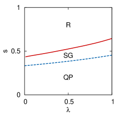
Second, the Hopfield model with two-body interactions and extensively many patterns is analyzed.
The difference from the previous case is that the SG phase appears owing to the many unretrieved patterns.
The spins in the SG phase tend to align in the direction, but do not correlate with any embedded patterns.
We have used the Suzuki-Trotter decomposition, the mean-field analysis, the replica trick, and the static ansatz to study the phase diagram.
The analysis within the RS solution has derived the phase diagram including three phases: the QP phase, the SG phase, and the R phase.
Although the phase boundary between the QP phase and the SG phase is of second order, the boundary between the SG phase and the R phase stays always of first order.
This result indicates difficulties for QA with antiferromagnetic transverse interactions.
Once the system is trapped in a basin in the SG phase, it is hard to escape there to reach the true ground state.
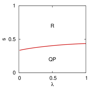
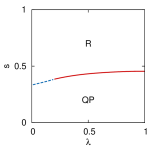
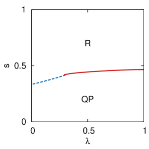
Finally, we have investigated the generalized Hopfield model with many-body interactions and extensively many patterns.
The resulting phase diagram consists of the QP and R phases.
Although the SG solution exists, it has a higher free energy than the other states.
We have confirmed that the first-order phase boundary vanishes at certain values of for and .
Hence, it is possible to avoid the difficulty of exponentially long running time of QA that results from a first-order phase transition.
In conclusion, we have revealed that antiferromagnetic transverse interactions improve the efficiency of QA for some random spin systems.
Using quantum fluctuations other than those induced by a transverse field is helpful for solving combinatorial optimization problems with QA.
In the present paper, we have investigated the efficiency of QA only for the Hopfield model.
It is an interesting problem to identify the class of problems that can be solved by QA with antiferromagnetic transverse interactions.
Appendix A Self-consistent equations for the Hopfield model with many-body interactions and finite patterns embedded
We derive the self-consistent equations (8) and (9) by mean-field analyses.
The Suzuki-Trotter formula and the static ansatz enable us to obtain the partition function.
Then, using a saddle-point condition, we obtain the self-consistent equations.
Let us calculate the partition function.
We first translate the quantum system into a classical system using the Suzuki-Trotter formula [26].
The Hamiltonian is given as
|
|
|
|
|
|
|
|
(30) |
where denotes an integer for the degree of interactions, and ’s the random variables.
The variable is an integer independent of .
Using the Trotter decomposition, and introducing closure relations, we have the following expression of the partition function for a finite Trotter number ,
|
|
|
|
|
|
|
|
(31) |
Here, denotes the summation over all possible spin configurations of and satisfying periodic boundary conditions, for all .
We next linearize the spin-product terms by using delta functions,
|
|
|
|
(32) |
and
|
|
|
|
(33) |
Then, Eq. (31) reads
|
|
|
|
|
|
|
|
|
|
|
|
|
|
|
|
|
|
|
|
(34) |
In the thermodynamic limit , according to the law of large numbers, the summation over the site index becomes the average over the randomness of the embedded patterns.
We refer to this average as the configurational average.
Furthermore, the integrals are evaluated by the saddle-point method.
The saddle-point conditions for and lead to
|
|
|
|
(35) |
and
|
|
|
|
(36) |
respectively.
Using the static ansatz, i.e., neglecting the -dependence of the order parameters, we can take the trace in Eq. (34) with the inverse operation of the Trotter decomposition.
We thus obtain the following partition function:
|
|
|
|
|
|
|
|
(37) |
where the brackets denote the configurational average.
Therefore the pseudo free energy is
|
|
|
|
|
|
|
|
|
(38) |
and the self-consistent equations are
|
|
|
|
|
|
|
|
(39) |
and
|
|
|
|
|
|
|
|
(40) |
In the low-temperature limit , the pseudo free energy and the self-consistent equations become
|
|
|
|
|
|
|
|
(41) |
and
|
|
|
|
(42) |
|
|
|
|
(43) |
Appendix B Self-consistent equations for the Hopfield model with many patterns
We derive the self-consistent equations for the Hopfield model with an extensive number of patterns embedded (16)–(20).
We closely follow Chap. 10 of Ref. [25] in the calculation.
The calculation uses the replica trick for configurational average.
Let us calculate the partition function.
In a similar way to the derivation of Eq. (34), the replicated partition function for a Trotter number is written as
|
|
|
|
|
|
|
|
|
|
|
|
|
|
|
|
|
|
|
|
(44) |
where represents the Trotter index, and the replica index.
We have used a Gaussian integral, instead of the delta function, to linearize the spin-product term regarding .
We consider the case where only a single pattern has a non-vanishing overlap with the state of the system: .
The overlap with the other patterns results from coincidental contributions, hence for .
Expanding the configurational average for in , we have
|
|
|
|
(45) |
Consequently, the term involving for in Eq. (44) is expressed as a quadratic form:
|
|
|
(46) |
with a matrix ,
|
|
|
|
(47) |
The integral with regard to for yields
|
|
|
|
(48) |
where we have defined the set of eigenvalues of as .
To linearize the spin-product term in , we replace the matrix by
|
|
|
|
(49) |
with the constraint
|
|
|
(50) |
|
|
|
(51) |
introduced by delta functions:
|
|
|
|
|
|
(52) |
|
|
|
|
|
|
(53) |
Thus, we can rewrite Eq. (44) as
|
|
|
|
|
|
|
|
|
|
|
|
|
|
|
|
|
|
|
|
|
|
|
|
(54) |
Here, denotes , and all the possible combinations of , , , and except for the case of .
We can take the trace in (54) independent of .
As a result, Eq. (54) reads
, where
|
|
|
|
|
|
|
|
|
|
|
|
|
|
|
|
|
|
|
|
|
|
|
|
(55) |
The saddle-point conditions for , , , and lead to the following self-consistent equations:
|
|
|
|
(56) |
|
|
|
|
(57) |
|
|
|
|
(58) |
|
|
|
|
(59) |
where the brackets mean the average with respect to the weight
|
|
|
|
|
|
|
|
|
(60) |
We look for the replica symmetric (RS) solution of Eqs. (56)–(59).
Furthermore, we use the static ansatz, that is, we neglect the dependence of the order parameters on the Trotter number:
|
|
|
|
|
|
|
|
(61) |
|
|
|
|
|
|
|
|
|
|
|
|
First, we evaluate the trace in Eq. (55).
Linearizing the spin-product term by using a Gaussian integral, we can rewrite the term including trace as
|
|
|
|
|
|
(62) |
where denotes the Gaussian measure , and is defined similarly.
Let us take the limit .
Using the inverse operation of the Trotter decomposition, we have
|
|
|
(63) |
The values of the integral are the same for both cases and , since the value is invariant under the variable transformation and .
Hence, Eq. (63) reads
|
|
|
(64) |
Next, we study the eigenvalues of .
The matrix has three types of elements:
|
|
|
|
(65) |
We can easily find that the matrix has the eigenvalues:
|
|
|
|
(66) |
with degeneracy , and
|
|
|
|
(67) |
with degeneracy , and
|
|
|
|
(68) |
with degeneracy .
Hence, the eigenvalue sum in Eq. (55) reads
|
|
|
(69) |
The pseudo free energy is given by using the replica trick:
|
|
|
|
(70) |
From the above results, we obtain
|
|
|
|
|
|
|
|
|
|
|
|
(71) |
In what follows, we will derive self-consistent equations in the low-temperature limit.
To simplify expressions shown later, we define the followings:
|
|
|
|
(72) |
|
|
|
|
(73) |
|
|
|
|
(74) |
The saddle-point conditions for the pseudo free energy (71) leads to the self-consistent equations
|
|
|
|
(75) |
|
|
|
|
(76) |
|
|
|
|
(77) |
|
|
|
|
(78) |
|
|
|
|
(79) |
|
|
|
|
(80) |
|
|
|
|
(81) |
The order parameter is greater than or equal to , since
|
|
|
|
|
|
|
|
|
|
|
|
|
|
|
|
|
|
|
|
|
|
|
|
(82) |
In particular, is equal to in the limit as shown below.
Assuming that , we have from Eqs. (80) and (81).
Then, Eqs. (77) and (78) read
|
|
|
|
(83) |
|
|
|
|
(84) |
which is in conflict with the assumption.
Hence, the relation holds in the low-temperature limit.
From Eq. (81), we have .
It follows that the integrands in the self-consistent equations are independent of ; the integrals with respect to are taken easily.
Consequently, the self-consistent equations in the low-temperature limit are
|
|
|
|
(85) |
|
|
|
|
(86) |
|
|
|
|
(87) |
Although is equal to , the factor converges to
|
|
|
|
(88) |
For this reason, we obtain
|
|
|
|
(89) |
The pseudo free energy is written as
|
|
|
|
|
|
|
|
(90) |
Appendix C Self-consistent equations for the Hopfield model with many-body interactions and with many patterns
We derive Eqs. (25)–(27) in this Appendix.
We closely follow the calculation in Ref. [23].
The target Hamiltonian is given by Eq. (4) and (5).
The number of patterns must be so that the free energy is extensive.
We consider the case where the system has a single non-vanishing overlap again.
The replicated partition function for a Trotter number is calculated in the same way as in the case of except that the spin-product term for is linearized by using the delta function:
|
|
|
|
|
|
|
|
|
|
|
|
|
|
|
|
|
|
|
|
|
|
|
|
(91) |
Note that only the spin-product term for the pattern with non-vanishing overlap is linearized.
The other spin-product term is evaluated as follows.
Expanding the exponential, we find that the linear term in the series vanishes.
The contribution from the second term is
|
|
|
|
|
|
|
|
|
(92) |
Since the contribution from the th term is of the order of , the correction to the term in the series, , is the greater one of and : For , , and for , .
Thus, the series reads
|
|
|
|
|
|
|
|
|
(93) |
Here, we have used .
The correction term is for , and for ; hence, this term is negligible in the thermodynamic limit.
Linearizing the spin-product term in Eq. (93) by using the delta functions (52) and (53), we can write the integrand in as with
|
|
|
|
|
|
|
|
|
|
|
|
|
|
|
|
|
|
|
|
|
|
|
|
|
|
|
|
(94) |
In a similar manner to the case of , we look for the RS solution, and use the static ansatz.
The spin-product term in Eq. (94) is linearized by using a Gaussian integral.
Expanding the configurational term in Eq. (94) in powers of , we have,
|
|
|
|
|
|
|
|
|
(95) |
The inverse operation of the Trotter decomposition leads to
|
|
|
(96) |
Using the replica trick, we finally obtain the following pseudo free energy:
|
|
|
|
|
|
|
|
|
|
|
|
(97) |
The saddle-point conditions for the pseudo free energy (97) yield the self-consistent equations.
Let
|
|
|
(98) |
and in the same way as in Eq. (73), and as in Eq. (74).
Then the self-consistent equations are given by Eqs. (75)–(79) with Eq. (98) and
|
|
|
|
(99) |
|
|
|
|
(100) |
In the same way as the case of , we find .
If , the free energy diverges in the limit .
Accordingly, must be equal to .
It follows that , so that the integrands in the self-consistent equations are independent of .
Hence, the self-consistent equations in the low-temperature limit are
|
|
|
|
(101) |
|
|
|
|
(102) |
|
|
|
|
(103) |
The factor converges to
|
|
|
|
(104) |
Since the factor converges to , the pseudo free energy in the low-temperature limit is
|
|
|
|
|
|
|
|
(105) |