On the scalar consistency relation away from slow roll

Abstract

As is well known, the non-Gaussianity parameter $f_{{}_{\rm NL}}$, which is often used to characterize the amplitude of the scalar bi-spectrum, can be expressed completely in terms of the scalar spectral index $n_{\rm s}$ in the squeezed limit, a relation that is referred to as the consistency condition. This relation, while it is largely discussed in the context of slow roll inflation, is actually expected to hold in any single field model of inflation, irrespective of the dynamics of the underlying model, provided inflation occurs on the attractor at late times. In this work, we explicitly examine the validity of the consistency relation, analytically as well as numerically, away from slow roll. Analytically, we first arrive at the relation in the simple case of power law inflation. We also consider the non-trivial example of the Starobinsky model involving a linear potential with a sudden change in its slope (which leads to a brief period of fast roll), and establish the condition completely analytically. We then numerically examine the validity of the consistency relation in three inflationary models that lead to the following features in the scalar power spectrum due to departures from slow roll: (i) a sharp cut off at large scales, (ii) a burst of oscillations over an intermediate range of scales, and (iii) small, but repeated, modulations extending over a wide range of scales. It is important to note that it is exactly such spectra that have been found to lead to an improved fit to the CMB data, when compared to the more standard power law primordial spectra, by the Planck team. We evaluate the scalar bi-spectrum for an arbitrary triangular configuration of the wavenumbers in these inflationary models and explicitly illustrate that, in the squeezed limit, the consistency condition is indeed satisfied even in situations consisting of strong deviations from slow roll. We conclude with a brief discussion of the results.

1 Introduction

Over the past two decades, cosmologists have dedicated a considerable amount of attention to hunting down credible models of inflation. The inflationary scenario, which is often invoked to resolve certain puzzles (such as the horizon problem) that plague the hot big bang model, is well known to provide an attractive mechanism for the origin of perturbations in the early universe [1, 2, 3]. In the modern viewpoint, it is the primordial perturbations generated during inflation that leave their signatures as anisotropies in the Cosmic Microwave Background (CMB) and later lead to the formation of the large scale structure. Ever since the discovery of the CMB anisotropies by COBE [4], there has been a constant endeavor to utilize cosmological observations to arrive at stronger and stronger constraints on models of inflation. While the CMB anisotropies have been measured with ever increasing precision by missions such as WMAP [5, 6, 7], Planck [8, 9, 10] and, very recently, by BICEP2 [11, 12], it would be fair to say that we still seem rather far from converging on a small class of well motivated and viable inflationary models (in this context, see Refs. [13, 14, 15]).

The difficulty in arriving at a limited set of credible models of inflation seems to lie in the simplicity and efficiency of the inflationary scenario. Inflation can be easily achieved with the aid of one or more scalar fields that are slowly rolling down a relatively flat potential. Due to this reason, a plethora of models of inflation have been proposed, which give rise to the required $60$ or so e-folds of accelerated expansion that is necessary to overcome the horizon problem. Moreover, there always seem to exist sufficient room to tweak the potential parameters in such a way so as to result in a nearly scale invariant power spectrum of the scalar perturbations that lead to a good fit to the CMB data. In such a situation, non-Gaussianities in general and the scalar bi-spectrum in particular have been expected to lift the degeneracy prevailing amongst the various inflationary models. For convenience, the extent of non-Gaussianity associated with the scalar bi-spectrum is often expressed in terms of the parameter commonly referred to as $f_{{}_{\rm NL}}$ [16], a quantity which is a dimensionless ratio of the scalar bi-spectrum to the power spectrum. The expectation regarding non-Gaussianities alluded to above has been largely corroborated by the strong limits that have been arrived at by the Planck mission on the value of the $f_{{}_{\rm NL}}$ parameter [17]. These bounds suggest that the observed perturbations are consistent with a Gaussian primordial distribution. Also, the strong constraints imply that exotic models which lead to large levels of non-Gaussianities are ruled out by the data.

Despite the strong bounds that have been arrived at on the amplitude of the scalar bi-spectrum, there exist many models of inflation that remain consistent with the cosmological data at hand. The so-called scalar consistency relation is expected to play a powerful role in this regard, ruling out, for instance, many multi-field models of inflation, if it is confirmed observationally (for early discussion in this context, see, for instance, Refs. [18, 19]; for recent discussions, see Refs. [20]; for similar results that involve the higher order correlation functions, see, for example, Refs. [21]). According to the consistency condition, in the squeezed limit of the three-point functions wherein one of the wavenumbers associated with the perturbations is much smaller than the other two, the three-point functions can be completely expressed in terms of the two-point functions. In the squeezed limit, for instance, the scalar non-Gaussianity parameter $f_{{}_{\rm NL}}$ can be expressed completely in terms of the scalar spectral index $n_{{}_{\rm S}}$ as $f_{{}_{\rm NL}}=5\,(n_{{}_{\rm S}}-1)/12$ [18, 19]. As we shall briefly outline later, the consistency conditions are expected to hold [27] whenever the amplitude of the perturbations freeze on super-Hubble scales, a behavior which is true in single field models where inflation occurs on the attractor at late times (see Refs. [1]; in this context, also see Refs. [28]). While the scalar consistency relation has been established in the slow roll scenario, we find that there has been only a limited effort in explicitly examining the relation in situations consisting of periods of fast roll [29, 30]. Moreover, it has been shown that there can be deviations from the consistency relation under certain conditions, particularly when the field is either evolving away from the attractor [31] or when the perturbations are in an excited state above the Bunch-Davies vacuum [32]. In this work, our aim is to verify the validity of the scalar consistency relation in inflationary models which exhibit non-trivial dynamics. By considering a few examples, we shall explicitly show, analytically and numerically, that the scalar consistency relation holds even in scenarios involving strong deviations from slow roll.

The remainder of this paper is organized as follows. In the next section, we shall quickly summarize a few essential points and results concerning the scalar power spectrum and the bi-spectrum. We shall also briefly revisit the proof of the scalar consistency relation in the squeezed limit. In the succeeding section, we shall explicitly verify the validity of the consistency condition analytically in the cases of power law inflation and the Starobinsky model which is described by a linear potential with a sudden change in its slope. We shall then evaluate the scalar bi-spectrum numerically for an arbitrary triangular configuration of the wavenumbers in three inflationary models that lead to features in the power spectrum, and examine the consistency condition in the squeezed limit. We conclude with a brief discussion on the results we obtain.

A few remarks on our conventions and notations seem essential at this stage of our discussion. We shall work with natural units wherein $\hbar=c=1$, and define the Planck mass to be $M_{{}_{\rm Pl}}=(8\,\pi\,G)^{-1/2}$. We shall adopt the signature of the metric to be $(-,+,+,+)$. We shall assume the background to be the spatially flat, Friedmann-Lemaître-Robertson-Walker (FLRW) line element that is described by the scale factor $a$ and the Hubble parameter $H$. As is convenient, we shall switch between various parametrizations of time, viz. the cosmic time $t$, the conformal time $\eta$ or e-folds denoted by $N$. An overdot and an overprime shall represent differentiation with respect to the cosmic and the conformal time coordinates, respectively. We shall restrict our attention in this work to inflationary models involving the canonical scalar field. Note that, in such a case, the first and second slow roll parameters are defined as $\epsilon_{1}=-\dot{H}/H^{2}$ and $\epsilon_{2}={\rm d}\ln\,\epsilon_{1}/{\rm d}N$.

2 The scalar bi-spectrum in the squeezed limit

In this section, we shall quickly summarize the essential definitions and governing expressions concerning the scalar power spectrum, the bi-spectrum and the corresponding non-Gaussianity parameter $f_{{}_{\rm NL}}$. We shall also sketch a simple proof of the consistency relation obeyed by the non-Gaussianity parameter $f_{{}_{\rm NL}}$ in the squeezed limit of the scalar bi-spectrum.

2.1 The scalar power spectrum and bi-spectrum

Consider the following line-element which describes the spatially flat, FLRW spacetime, when the scalar perturbations, characterized by the curvature perturbation ${\mathcal{R}}$, have been taken into account:

$${\rm d}s^{2}=-{\rm d}t^{2}+a^{2}(t)\;{\rm e}^{2\,{\cal R}(t,{\bm{x}})}{\rm d}{\bm{x}}^{2}.$$ (2.1)

Let $f_{k}$ denote the Fourier modes associated with the curvature perturbation at the linear order in the perturbations. In the case of inflation driven by the canonical scalar field that is of our interest here, the modes $f_{k}$ satisfy the differential equation [2, 3]

$$f_{k}^{\prime\prime}+2\,\frac{z^{\prime}}{z}\,f_{k}^{\prime}+k^{2}\,f_{k}=0,$$ (2.2)

where $z=\sqrt{2\,\epsilon_{1}}\,M_{{}_{\rm Pl}}\,a$. Upon quantization, the curvature perturbation can be decomposed in terms of the Fourier modes $f_{k}$ as

$${\hat{\mathcal{R}}}(\eta,{\bm{x}})=\int\frac{{\rm d}^{3}{{\bm{k}}}}{(2\,\pi)^{3/2}}\,{\hat{\cal R}}_{{\bm{k}}}(\eta)\;{\rm e}^{i\,{\bm{k}}\cdot{\bm{x}}}=\int\frac{{\rm d}^{3}{{\bm{k}}}}{(2\,\pi)^{3/2}}\,\left[{\hat{a}}_{{\bm{k}}}\,f_{k}(\eta)\,{\rm e}^{i\,{\bm{k}}\cdot{\bm{x}}}+{\hat{a}}_{{\bm{k}}}^{\dagger}\,f_{k}^{\ast}(\eta)\,{\rm e}^{-i\,{\bm{k}}\cdot{\bm{x}}}\right],$$ (2.3)

where ${\hat{a}}_{{\bm{k}}}$ and ${\hat{a}}_{{\bm{k}}}^{\dagger}$ are the usual creation and annihilation operators that obey the standard commutation relations.

The scalar power spectrum ${\cal P}_{{}_{\rm S}}(k)$ is defined in terms of the two-point correlation function of the curvature perturbation as follows:

$$\langle 0|{\hat{\mathcal{R}}}_{{\bm{k}}}(\eta)\,{\hat{\mathcal{R}}}_{{\bm{k}}^{\prime}}(\eta)|0\rangle=\frac{(2\,\pi)^{2}}{2\,k^{3}}\;{\cal P}_{{}_{\rm S}}(k)\;\delta^{(3)}\left({\bm{k}}+{\bm{k}}^{\prime}\right),$$ (2.4)

where $|0\rangle$ denotes the Bunch-Davies vacuum annihilated by the operator ${\hat{a}}_{{\bm{k}}}$ [33]. In terms of the modes $f_{k}$, the scalar power spectrum ${\cal P}_{{}_{\rm S}}(k)$ is given by

$${\cal P}_{{}_{\mathrm{S}}}(k)=\frac{k^{3}}{2\,\pi^{2}}\,|f_{k}|^{2}.$$ (2.5)

The inflationary model governed by a given potential determines the behavior of the quantity $z$. In order to arrive at the scalar power spectrum using the above expression, one first solves the differential equation (2.2) for the modes $f_{k}$ with the Bunch-Davies initial conditions [33], and then evaluates the amplitude of the modes at sufficiently late times when they are well outside the Hubble radius during inflation. The scalar spectral index is defined as

$$n_{{}_{\rm S}}(k)=1+\frac{{\rm d}\ln{\mathcal{P}}_{{}_{\rm S}}(k)}{{\rm d}\ln k}.$$ (2.6)

It should be stressed here that the scalar spectral index proves to be a constant only in simple situations such as power law and slow roll inflation. In general, when the power spectrum contains features, the quantity $n_{{}_{\rm S}}$ depends on the wavenumber $k$.

The scalar bi-spectrum ${\cal B}_{{}_{\rm S}}({\bm{k}}_{1},{\bm{k}}_{2},{\bm{k}}_{3})$ evaluated, say, in the vacuum state $|0\rangle$, is defined in terms of the three-point function of the curvature perturbation as follows [6]:

$$\langle 0|{\hat{\mathcal{R}}}_{{\bm{k}}_{1}}\,{\hat{\mathcal{R}}}_{{\bm{k}}_{2}}\,{\hat{\mathcal{R}}}_{{\bm{k}}_{3}}|0\rangle=\left(2\,\pi\right)^{3}\,{\cal B}_{{}_{\rm S}}({\bm{k}}_{1},{\bm{k}}_{2},{\bm{k}}_{3})\;\delta^{(3)}\left({\bm{k}}_{1}+{\bm{k}}_{2}+{\bm{k}}_{3}\right).$$ (2.7)

Note that the delta function on the right hand side imposes the triangularity condition, viz. that the three wavevectors ${\bm{k}}_{1}$, ${\bm{k}}_{2}$ and ${\bm{k}}_{3}$ have to form the edges of a triangle. For the sake of convenience, we shall set

$${\cal B}_{{}_{\mathrm{S}}}({\bm{k}}_{1},{\bm{k}}_{2},{\bm{k}}_{3})=\left(2\,\pi\right)^{-9/2}\;G({\bm{k}}_{1},{\bm{k}}_{2},{\bm{k}}_{3}).$$ (2.8)

The non-Gaussianity parameter $f_{{}_{\rm NL}}$ that is often used to characterize the extent of non-Gaussianity indicated by the bi-spectrum is introduced through the relation [16]

$${\mathcal{R}}(\eta,{\bm{x}})={\mathcal{R}}_{{}_{\mathrm{G}}}(\eta,{\bm{x}})-\frac{3\,f_{{}_{\rm NL}}}{5}\,\left[{\mathcal{R}}_{{}_{\mathrm{G}}}^{2}(\eta,{\bm{x}})-\left\langle{\mathcal{R}}_{{}_{\mathrm{G}}}^{2}(\eta,{\bm{x}})\right\rangle\right],$$ (2.9)

where ${\mathcal{R}}_{{}_{\mathrm{G}}}$ denotes the Gaussian part of the curvature perturbation. Using the above relation and Wick’s theorem (which applies to Gaussian perturbations), one can arrive at the following expression for the dimensionless non-Gaussianity parameter $f_{{}_{\rm NL}}$ in terms of the bi-spectrum $G({\bm{k}}_{1},{\bm{k}}_{2},{\bm{k}}_{3})$ and the scalar power spectrum ${\cal P}_{{}_{\mathrm{S}}}(k)$:

$$f_{{}_{\rm NL}}({\bm{k}}_{1},{\bm{k}}_{2},{\bm{k}}_{3}) = -\frac{10}{3}\;\frac{1}{(2\,\pi)^{4}}\;\left(k_{1}\,k_{2}\,k_{3}\right)^{3}\;G({\bm{k}}_{1},{\bm{k}}_{2},{\bm{k}}_{3})$$ (2.10)

$$\times\left[k_{1}^{3}\;{\cal P}_{{}_{\rm S}}(k_{2})\;{\cal P}_{{}_{\rm S}}(k_{3})+{\rm two~{}permutations}\right]^{-1}.$$

The scalar bi-spectrum generated during inflation can be evaluated using the Maldacena formalism [18]. The approach basically makes use of the third order action governing the curvature perturbation and the standard rules of perturbative quantum field theory to arrive at the scalar three-point function [18, 34, 35]. It is found that, in the case of inflation driven by the canonical scalar field, the third order action consists of six terms and the scalar bi-spectrum receives a contribution from each of these ‘vertices’. In fact, there also occurs a seventh term which arises due to a field redefinition, a procedure which is necessary to reduce the action to a simpler form. One can show that the complete contribution to the scalar bi-spectrum in the perturbative vacuum can be written as [36, 37, 38]

$$G({\bm{k}}_{1},{\bm{k}}_{2},{\bm{k}}_{3}) \equiv \sum_{C=1}^{7}\;G_{{}_{C}}({\bm{k}}_{1},{\bm{k}}_{2},{\bm{k}}_{3})$$ (2.11)

$$\equiv M_{{}_{\rm Pl}}^{2}\;\sum_{C=1}^{6}\;\Biggl{\{}\left[f_{k_{1}}(\eta_{\rm e})\,f_{k_{2}}(\eta_{\rm e})\,f_{k_{3}}(\eta_{\rm e})\right]\;{\cal G}_{{}_{C}}({\bm{k}}_{1},{\bm{k}}_{2},{\bm{k}}_{3})$$

$$+\left[f_{k_{1}}^{\ast}(\eta_{\rm e})\,f_{k_{2}}^{\ast}(\eta_{\rm e})\,f_{k_{3}}^{\ast}(\eta_{\rm e})\right]\;{\cal G}_{{}_{C}}^{\ast}({\bm{k}}_{1},{\bm{k}}_{2},{\bm{k}}_{3})\Biggr{\}}$$

$$+\,G_{7}({\bm{k}}_{1},{\bm{k}}_{2},{\bm{k}}_{3}),$$

where $f_{k}$ are the Fourier modes in terms of which we had decomposed the curvature perturbation at the linear order in the perturbations [cf. Eq. (2.3)]. In the above expression, the quantities ${\cal G}_{{}_{C}}({\bm{k}}_{1},{\bm{k}}_{2},{\bm{k}}_{3})$ with $C=(1,6)$ correspond to the six vertices in the interaction Hamiltonian (obtained from the third order action), and are described by the integrals

$${\cal G}_{1}({\bm{k}}_{1},{\bm{k}}_{2},{\bm{k}}_{3}) = 2\,i\,\int_{\eta_{\rm i}}^{\eta_{\rm e}}{\rm d}\eta\;a^{2}\,\epsilon_{1}^{2}\,\left(f_{k_{1}}^{\ast}\,f_{k_{2}}^{\prime\ast}\,f_{k_{3}}^{\prime\ast}+{\rm two~{}permutations}\right),$$ (2.12a)

$${\cal G}_{2}({\bm{k}}_{1},{\bm{k}}_{2},{\bm{k}}_{3}) = -2\,i\;\left({\bm{k}}_{1}\cdot{\bm{k}}_{2}+{\rm two~{}permutations}\right)\;\int_{\eta_{\rm i}}^{\eta_{\rm e}}{\rm d}\eta\;a^{2}\,\epsilon_{1}^{2}\,f_{k_{1}}^{\ast}\,f_{k_{2}}^{\ast}\,f_{k_{3}}^{\ast},$$ (2.12b)

$${\cal G}_{3}({\bm{k}}_{1},{\bm{k}}_{2},{\bm{k}}_{3}) = -2\,i\,\int_{\eta_{\rm i}}^{\eta_{\rm e}}{\rm d}\eta\;a^{2}\,\epsilon_{1}^{2}\;\Biggl{[}\left(\frac{{\bm{k}}_{1}\cdot{\bm{k}}_{2}}{k_{2}^{2}}\right)\,f_{k_{1}}^{\ast}\,f_{k_{2}}^{\prime\ast}\,f_{k_{3}}^{\prime\ast}+{\rm five~{}permutations}\Biggr{]},\quad$$ (2.12c)

$${\cal G}_{4}({\bm{k}}_{1},{\bm{k}}_{2},{\bm{k}}_{3}) = i\,\int_{\eta_{\rm i}}^{\eta_{\rm e}}{\rm d}\eta\;a^{2}\,\epsilon_{1}\,\epsilon_{2}^{\prime}\,\left(f_{k_{1}}^{\ast}\,f_{k_{2}}^{\ast}\,f_{k_{3}}^{\prime\ast}+{\rm two~{}permutations}\right),$$ (2.12d)

$${\cal G}_{5}({\bm{k}}_{1},{\bm{k}}_{2},{\bm{k}}_{3}) = \frac{i}{2}\,\int_{\eta_{\rm i}}^{\eta_{\rm e}}{\rm d}\eta\;a^{2}\,\epsilon_{1}^{3}\;\Biggl{[}\left(\frac{{\bm{k}}_{1}\cdot{\bm{k}}_{2}}{k_{2}^{2}}\right)\,f_{k_{1}}^{\ast}\,f_{k_{2}}^{\prime\ast}\,f_{k_{3}}^{\prime\ast}+{\rm five~{}permutations}\Biggr{]},$$ (2.12e)

$${\cal G}_{6}({\bm{k}}_{1},{\bm{k}}_{2},{\bm{k}}_{3}) = \frac{i}{2}\,\int_{\eta_{\rm i}}^{\eta_{\rm e}}{\rm d}\eta\;a^{2}\,\epsilon_{1}^{3}\;\Biggl{\{}\left[\frac{k_{1}^{2}\,\left({\bm{k}}_{2}\cdot{\bm{k}}_{3}\right)}{k_{2}^{2}\,k_{3}^{2}}\right]\,f_{k_{1}}^{\ast}\,f_{k_{2}}^{\prime\ast}\,f_{k_{3}}^{\prime\ast}+{\rm two~{}permutations}\Biggr{\}}.\qquad$$ (2.12f)

These integrals are to be evaluated from a sufficiently early time, say, $\eta_{\rm i}$, when the initial conditions are imposed on the modes until very late times, say, towards the end of inflation at $\eta_{\rm e}$. The additional, seventh term $G_{7}({\bm{k}}_{1},{\bm{k}}_{2},{\bm{k}}_{3})$ arises due to the field redefinition and its contribution to the bi-spectrum $G({\bm{k}}_{1},{\bm{k}}_{2},{\bm{k}}_{3})$ is given by

$$G_{7}({\bm{k}}_{1},{\bm{k}}_{2},{\bm{k}}_{3})=\frac{\epsilon_{2}(\eta_{\rm e})}{2}\,\left(|f_{k_{1}}(\eta_{\rm e})|^{2}\,|f_{k_{2}}(\eta_{\rm e})|^{2}+{\rm two~{}permutations}\right).$$ (2.13)

2.2 The consistency relation

The squeezed limit refers to the case wherein one of the wavenumbers of the triangular configuration vanishes, say, $k_{3}\to 0$, leading to ${\bm{k}}_{2}=-{\bm{k}}_{1}$. Or, equivalently, one of the modes is assumed to possess a wavelength which is much larger than the other two. The long wavelength mode would be well outside the Hubble radius. In models of inflation driven by a single scalar field, the amplitude of the curvature perturbation freezes on super-Hubble scales, provided the inflaton evolves on the attractor at late times [28, 31]. As a result, the long wavelength mode simply acts as a background as far as the other two modes are concerned. If ${\cal R}^{{}_{{}^{{}^{\rm B}}}}$ is the amplitude of the curvature perturbation associated with the long wavelength mode, then the unperturbed part of the original FLRW metric will be modified to

$${\rm d}s^{2}=-{\rm d}t^{2}+a^{2}(t)\,{\rm e}^{2\,{\cal R}^{{}_{{{}^{\rm B}}}}}\,{\rm d}{\bm{x}}^{2}.$$ (2.14)

In other words, the effect of the long wavelength mode is to modify the scale factor locally, which is equivalent to a spatial transformation of the form ${\bm{x}^{\prime}}=\Lambda\,{\bm{x}}$, with the components of the matrix $\Lambda$ being given by $\Lambda_{ij}={\rm e}^{{\cal R}^{{}_{{{}^{\rm B}}}}}\,\delta_{ij}$. Under such a transformation, the modes of the curvature perturbation transform as ${\mathcal{R}}_{\bm{k}}\to{\rm det}~{}(\Lambda^{-1})\,{\cal R}_{\Lambda^{-1}{\bm{k}}}$. Further, we have $|\Lambda^{-1}\,{\bm{k}}|=(1-{\cal R}^{{}_{{}^{{}^{\rm B}}}})\;k$ and $\delta^{(3)}(\Lambda^{-1}\,{\bm{k}}_{1}+\Lambda^{-1}\,{\bm{k}}_{2})={\rm det}~{}(\Lambda)\;\delta^{(3)}({\bm{k}}_{1}+{\bm{k}}_{2})$. Utilizing these relations, the scalar two-point function can be written as

$$\langle\hat{{\mathcal{R}}}_{{\bm{k}}_{1}}\,\hat{{\mathcal{R}}}_{{\bm{k}}_{2}}\rangle_{k} = \frac{(2\,\pi)^{2}}{2\,k_{1}^{3}}\;{\mathcal{P}}_{{}_{\rm S}}(k_{1})\;\left[1-(n_{{}_{\rm S}}-1)\,{\cal R}^{{}_{{}^{{}^{\rm B}}}}\right]\,\delta^{(3)}({\bm{k}}_{1}+{\bm{k}}_{2}),$$ (2.15)

where the suffix $k$ on the two-point function indicates that the correlator has been evaluated in the presence of a long wavelength perturbation. Upon using the above expression for the scalar power spectrum, we can write the scalar bi-spectrum in the squeezed limit as [19, 26, 27]

$$\langle\,\hat{{\mathcal{R}}}_{{\bm{k}}_{1}}\,\hat{{\mathcal{R}}}_{{\bm{k}}_{2}}\,\hat{{\mathcal{R}}}_{{\bm{k}}_{3}}\,\rangle_{k_{3}} \equiv \langle\,\langle\,\hat{\cal R}_{{\bm{k}}_{1}}\,\hat{\cal R}_{{\bm{k}}_{2}}\,\rangle_{k_{3}}\;\hat{\cal R}_{{\bm{k}}_{3}}\,\rangle$$ (2.16)

$$= -\,\frac{(2\,\pi)^{5/2}}{4\,k_{1}^{3}\,k_{3}^{3}}\,\left(n_{{}_{\rm S}}-1\right)\,{\mathcal{P}}_{{}_{\rm S}}(k_{1})\,{\mathcal{P}}_{{}_{\rm S}}(k_{3})\;\delta^{3}({\bm{k}}_{1}+{\bm{k}}_{2}).$$

On making use of this expression for the scalar bi-spectrum in the squeezed limit and the definition of the scalar power spectrum, one can immediately arrive at the consistency relation for $f_{{}_{\rm NL}}$, viz. that $f_{{}_{\rm NL}}=5\,(n_{{}_{\rm S}}-1)/12$ [18, 19, 20].

3 Analytically examining the validity of the condition away from slow roll

As was outlined in the previous section, the only requirement for the validity of the consistency relation is the existence of a unique clock during inflation. Hence, in principle, this relation should be valid for any single field model of inflation irrespective of the detailed dynamics, if the field is evolving on the attractor at late times. Therefore, it should be valid even away from slow roll. In this section, we shall analytically examine the validity of the consistency condition in scenarios consisting of deviations from slow roll. After establishing the relation first in the simple case of power law inflation, we shall consider the Starobinsky model which involves a brief period of fast roll.

3.1 The simple example of power law inflation

We shall first consider the case of power law inflation with no specific constraints on the power law index, so that the behavior of the scale factor can be far different from that of its behavior in slow roll inflation. In power law inflation, the scale factor can be written as

$$a(\eta)=a_{1}\,\left(\frac{\eta}{\eta_{1}}\right)^{\gamma+1},$$ (3.1)

where $a_{1}$ and $\eta_{1}$ are constants, and $\gamma<-2$. In such a background, the Fourier modes $f_{k}$ associated with the curvature perturbation that satisfy the Bunch-Davies initial conditions are found to be [37, 39]

$$f_{k}(\eta)=\frac{1}{\sqrt{2\,\epsilon_{1}}\,M_{{}_{\rm Pl}}\,a(\eta)}\,\sqrt{\frac{-\pi\,\eta}{4}}\;{\rm e}^{-i\,\pi\,\gamma/2}\;H_{-(\gamma+1/2)}^{(1)}(-k\,\eta),$$ (3.2)

where the first slow roll parameter $\epsilon_{1}$ is a constant given by $\epsilon_{1}=(\gamma+2)/(\gamma+1)$. Note that $H_{\nu}^{(1)}(x)$ denotes the Hankel function of the first kind [40], while the scale factor $a(\eta)$ is given by Eq. (3.1). For real arguments, the Hankel functions of the first and the second kinds, viz. $H_{\nu}^{(1)}(x)$ and $H_{\nu}^{(2)}(x)$, are complex conjugates of each other [40]. Moreover, as $x\to 0$, the Hankel function has the following form

$$\lim_{x\rightarrow 0}\,H_{\nu}^{(1)}(x)=\frac{i}{\pi\,\nu}\,\left[\Gamma(1-\nu)\,{\rm e}^{-i\,\pi\,\nu}\,\left(\frac{x}{2}\right)^{\nu}-\Gamma(1+\nu)\,\left(\frac{x}{2}\right)^{-\nu}\right].$$ (3.3)

Upon using this behavior, one can show that the corresponding scalar power spectrum, evaluated at late times, i.e. as $\eta\to-0$, is given by

$${\mathcal{P}}_{{}_{\rm S}}(k)=\frac{1}{2\,\pi^{3}\,M_{{}_{\rm Pl}}^{2}\,\epsilon_{1}}\,\left(\frac{|\eta_{1}|^{\gamma+1}}{a_{1}}\right)^{2}\,\biggl{|}\Gamma[-(\gamma+1/2)]\biggr{|}^{2}\;\left(\frac{k}{2}\right)^{2\,(\gamma+2)},$$ (3.4)

where $\Gamma(x)$ represents the Gamma function [40]. The scalar spectral index corresponding to such a power spectrum is evidently a constant and can be easily determined to be $n_{{}_{\rm S}}=2\,\gamma+5$. If the consistency condition is true, it would then imply that the scalar non-Gaussianity parameter has the value $f_{{}_{\rm NL}}=5\,(\gamma+2)/6$ in the squeezed limit.

Let us now evaluate the scalar bi-spectrum in the squeezed limit using the Maldacena formalism and illustrate that it indeed leads to the above consistency condition for $f_{{}_{\rm NL}}$. It should be clear that, in order to arrive at the complete scalar bi-spectrum, we first need to carry out the integrals (2.12) associated with the six vertices, calculate the corresponding contributions $G_{{}_{C}}({\bm{k}}_{1},{\bm{k}}_{2},{\bm{k}}_{3})$ for $C=(1,6)$, and lastly add the contribution $G_{7}({\bm{k}}_{1},{\bm{k}}_{2},{\bm{k}}_{3})$ [cf. Eq. (2.13)] that arises due to the field redefinition. However, since $\epsilon_{1}$ is a constant in power law inflation, the second slow roll parameter $\epsilon_{2}$ vanishes identically. As a result, the contribution corresponding to the fourth term that is determined by the integral (2.12d) as well as the seventh term $G_{7}({\bm{k}}_{1},{\bm{k}}_{2},{\bm{k}}_{3})$ prove to be zero. Moreover, in the squeezed limit of our interest, i.e. as $k_{3}\to 0$, the amplitude of the mode $f_{k_{3}}$ freezes and hence its time derivative goes to zero. Therefore, terms that are either multiplied by the wavenumber corresponding to the long wavelength mode or explicitly involve the time derivative of the long wavelength mode do not contribute, as both vanish in the squeezed limit. Due to these reasons, one finds that it is only the first and the second terms, determined by the integrals (2.12a) and (2.12b), that contribute in power law inflation. After an integration by parts, we find that, in the squeezed limit, these two integrals can be combined to be expressed as

$$\lim_{k_{3}\to 0}\,\left[{\cal G}_{1}({\bm{k}},-{\bm{k}},{\bm{k}}_{3})+{\cal G}_{2}({\bm{k}},-{\bm{k}},{\bm{k}}_{3})\right]=\lim_{k_{3}\to 0}\,2\,i\,\epsilon_{1}^{2}\,f_{k_{3}}^{\ast}\,\left[\left(a^{2}\,f_{k}^{\prime\ast}\,f_{k}^{\ast}\right)_{-\infty}^{0}+2\,k^{2}\,\int_{-\infty}^{0}{\rm d}\eta\,a^{2}\,f_{k}^{\ast 2}\right],$$ (3.5)

where we have set $\eta_{\rm i}=-\infty$ and $\eta_{\rm e}=0$. One can show that the derivative $f_{k}^{\prime}$ can be written as

$$f_{k}^{\prime}(\eta)=\frac{-k}{\sqrt{2\,\epsilon_{1}}\,M_{{}_{\rm Pl}}\,a(\eta)}\,\sqrt{\frac{-\pi\,\eta}{4}}\;{\rm e}^{-i\,\pi\,\gamma/2}\,H_{-(\gamma+3/2)}^{(1)}(-k\,\eta).$$ (3.6)

Therefore, upon using this expression for the derivative $f_{k}^{\prime}$, the behavior (3.3), the following asymptotic form of the Hankel function

$$\lim_{x\rightarrow\infty}\,H_{\nu}^{(1)}(x)=\sqrt{\frac{2}{\pi\,x}}\,{\rm e}^{i\,(x-\pi\,\nu/2-\pi/4)},\\$$ (3.7)

and the integral [40]

$$\int{\rm d}x\,x\,\left[H_{\nu}^{(1)}(x)\right]^{2}=\frac{x^{2}}{2}\,\left\{\left[H_{\nu}^{(1)}(x)\right]^{2}-H_{\nu-1}^{(1)}(x)\,H_{\nu+1}^{(1)}(x)\right\},$$ (3.8)

we find that the bi-spectrum in the squeezed limit can be written as

$$\lim_{k_{3}\to 0}\,k^{3}\,k_{3}^{3}\,G({\bm{k}},-{\bm{k}},{\bm{k}}_{3})=-8\,\pi^{4}\,(\gamma+2)\,{\cal P}_{{}_{\rm S}}(k)\,{\cal P}_{{}_{\rm S}}(k_{3}).$$ (3.9)

This expression and the definition (2.10) for the scalar non-Gaussianity parameter then leads to $f_{{}_{\rm NL}}=5\,(\gamma+2)/6$, which is the result suggested by the consistency relation. We should add here that such a result has been arrived at earlier using a slightly different approach (see the third reference in Refs. [20]).

3.2 A non-trivial example involving the Starobinsky model

The second example that we shall consider is the Starobinsky model. In the Starobinsky model, the inflaton rolls down a linear potential which changes its slope suddenly at a particular value of the scalar field [41]. The governing potential is given by

$$V(\phi)=\left\{\begin{array}[]{rcl}V_{0}+A_{+}\,(\phi-\phi_{0})&{\rm for}&\phi>\phi_{0},\\ V_{0}+A_{-}\,(\phi-\phi_{0})&{\rm for}&\phi<\phi_{0},\end{array}\right.$$ (3.10)

where $V_{0}$, $A_{+}$, $A_{-}$ and $\phi_{0}$ are constants. An important aspect of the Starobinsky model is the assumption that it is the constant $V_{0}$ which dominates the value of the potential around $\phi_{0}$. Due to this reason, the scale factor always remains rather close to that of de Sitter. This in turn implies that the first slow roll parameter $\epsilon_{1}$ remains small throughout the domain of interest. However, the discontinuity in the slope of the potential at $\phi_{0}$ causes a transition to a brief period of fast roll before slow roll is restored at late times. One finds that the transition leads to large values for the second slow roll parameter $\epsilon_{2}$ and, importantly, the quantity $\dot{\epsilon}_{2}$ grows to be even larger, in fact, behaving as a Dirac delta function at the transition. As we shall discuss, it is this behavior that leads to the most important contribution to the scalar bi-spectrum in the model [36, 42, 43].

Clearly, it would be convenient to divide the evolution of the background quantities and the perturbation variables into two phases, before and after the transition at $\phi_{0}$. In what follows, we shall represent the various quantities corresponding to the epochs before and after the transition by a plus sign and a minus sign (in the super-script or sub-script, as is convenient), while the values of the quantities at the transition will be denoted by a zero. Let us quickly list out the behavior of the different quantities which we shall require to establish the consistency relation.

The first slow roll parameter before and after the transition is found to be [41, 36, 42, 43]

$$\epsilon_{1+}(\eta) \simeq \frac{A_{+}^{2}}{18\,M_{{}_{\rm Pl}}^{2}\,H_{0}^{4}},$$ (3.11a)

$$\epsilon_{1-}(\eta) \simeq \frac{A_{-}^{2}}{18\,M_{{}_{\rm Pl}}^{2}\,H_{0}^{4}}\,\left[1-\frac{\Delta A}{A_{-}}\,\left(\frac{\eta}{\eta_{0}}\right)^{3}\right]^{2},$$ (3.11b)

where $\Delta A=A_{-}-A_{+}$, $H_{0}$ is the Hubble parameter determined by the relation $H_{0}^{2}\simeq V_{0}/(3\,M_{{}_{\rm Pl}}^{2})$, and $\eta_{0}$ denotes the conformal time when the transition takes place. The second slow roll parameter is given by

$$\epsilon_{2+}(\eta) = 4\,\epsilon_{1+},$$ (3.12a)

$$\epsilon_{2-}(\eta) = \frac{6\,\Delta\,A}{A_{-}}\,\frac{(\eta/\eta_{0})^{3}}{1\,-\,(\Delta\,A/A_{-})\,\left(\eta/\eta_{0}\right)^{3}}+4\,\epsilon_{1-}.$$ (3.12b)

In fact, to determine the modes associated with the scalar perturbations and to evaluate the dominant contribution to the scalar bi-spectrum, we shall also require the behavior of the quantity $\dot{\epsilon}_{2}$. One can show that $\dot{\epsilon}_{2}$ can be expressed as

$$\dot{\epsilon}_{2}=-\frac{2\,V_{\phi\,\phi}}{H}+12\,H\,\epsilon_{1}-3\,H\,\epsilon_{2}-4\,H\,\epsilon_{1}^{2}+5\,H\,\epsilon_{1}\epsilon_{2}-\frac{H}{2}\,\epsilon_{2}^{2},$$ (3.13)

where $V_{\phi\phi}={\rm d}^{2}V/{\rm d}\phi^{2}$, and it should be stressed that this is an exact relation. It should be clear that the first term in the above expression involving $V_{\phi\phi}$ will lead to a Dirac delta function due to the discontinuity in the first derivative of the potential in the case of the Starobinsky model. Hence, the dominant contribution to $\dot{\epsilon}_{2}$ at the transition can be written as [42, 43]

$$\dot{\epsilon}_{2}^{\,0}\simeq\frac{2\,\Delta\,A}{H_{0}}\,\delta^{(1)}(\phi\,-\,\phi_{0})=\frac{6\,\Delta\,A}{A_{+}\,a_{0}}\,\delta^{(1)}(\eta\,-\,\eta_{0}),$$ (3.14)

where $a_{0}$ denotes the value of the scale factor when $\eta=\eta_{0}$ . Post transition, the dominant contribution to $\dot{\epsilon}_{2}$ is found to be [36]

$$\dot{\epsilon}_{2-}\simeq-3\,H\,\epsilon_{2-}-\frac{H}{2}\,\epsilon_{2-}^{2}\simeq-\frac{18\,H_{0}\,\Delta\,A}{A_{-}}\,\frac{\left(\eta/\eta_{0}\right)^{3}}{\left[1-(\Delta\,A/A_{-})\,\left(\eta/\eta_{0}\right)^{3}\right]^{2}}.$$ (3.15)

Due to the fact that the potential is linear and also since the first slow roll parameter remains small, the modes $f_{k}$ governing the curvature perturbation can be described by the conventional de Sitter modes to a good approximation before the transition. For the same reasons, one finds that the scalar modes can be described by the de Sitter modes soon after the transition as well. However, due to the transition, the modes after the transition are related by the Bogoliubov transformations to the modes before the transition. Therefore, the scalar mode and its time derivative before the transition can be written as [41, 36, 44, 42, 43]:

$$f_{k}^{+}(\eta) = \frac{i\,H_{0}}{2\,M_{{}_{\rm Pl}}\,\sqrt{{k^{3}}\,\epsilon_{1+}}}\,\left(1+i\,k\,\eta\right)\,{\rm e}^{-i\,k\,\eta},$$ (3.16a)

$$f_{k}^{+}{}^{\prime}(\eta) = \frac{i\,H_{0}}{2\,M_{{}_{\rm Pl}}\,\sqrt{{k^{3}}\,\epsilon_{1+}}}\,\left[\frac{3\,\epsilon_{1+}}{\eta}\,\left(1+i\,k\,\eta\right)+k^{2}\,\eta\right]{\rm e}^{-i\,k\,\eta}.$$ (3.16b)

Whereas, the mode and its derivative after the transition can be expressed as follows:

$$f_{k}^{-}(\eta) = \frac{i\,H_{0}\,\alpha_{k}}{2\,M_{{}_{\rm Pl}}\,\sqrt{{k^{3}}\,\epsilon_{1-}}}\,\left(1+i\,k\,\eta\right)\,{\rm e}^{-i\,k\,\eta}-\frac{i\,H_{0}\,\beta_{k}}{2\,M_{{}_{\rm Pl}}\,\sqrt{{k^{3}}\,\epsilon_{1-}}}\left(1-i\,k\,\eta\right)\,{\rm e}^{i\,k\,\eta},$$ (3.17a)

$$f_{k}^{-}{}^{\prime}(\eta) = \frac{i\,H_{0}\,\alpha_{k}}{2\,M_{{}_{\rm Pl}}\,\sqrt{{k^{3}}\epsilon_{1-}}}\left[\left(\epsilon_{1-}+\frac{\epsilon_{2-}}{2}\right)\,\frac{1}{\eta}\,\left(1+i\,k\,\eta\right)+k^{2}\,\eta\right]\,{\rm e}^{-i\,k\,\eta}$$ (3.17b)

$$- \frac{i\,H_{0}\,\beta_{k}}{2\,M_{{}_{\rm Pl}}\,\sqrt{{k^{3}}\epsilon_{1-}}}\left[\left(\epsilon_{1-}+\frac{\epsilon_{2-}}{2}\right)\,\frac{1}{\eta}\,\left(1-i\,k\,\eta\right)+k^{2}\,\eta\right]{\rm e}^{i\,k\,\eta},$$

with $\alpha_{k}$ and $\beta_{k}$ denoting the Bogoliubov coefficients. Upon matching the above modes and their time derivatives at the transition, the Bogoliubov coefficients can be determined to be

$$\alpha_{k} = 1+\frac{3\,i\,\Delta A}{2\,A_{+}}\;\frac{k_{0}}{k}\,\left(1+\frac{k_{0}^{2}}{k^{2}}\right),$$ (3.18a)

$$\beta_{k} = -\frac{3\,i\,\Delta A}{2\,A_{+}}\;\frac{k_{0}}{k}\,\left(1+\frac{i\,k_{0}}{k}\right)^{2}\,{\rm e}^{2\,i\,k/k_{0}},$$ (3.18b)

where $k_{0}=-1/\eta_{0}=a_{0}\,H_{0}$ denotes the mode that leaves the Hubble radius at the transition. At late times, the scalar mode behaves as

$$f_{k}^{-}(\eta_{\rm e})=\frac{i\,H_{0}}{2\,M_{{}_{\rm Pl}}\,\sqrt{{k^{3}}\,\epsilon_{1-}(\eta_{\rm e})}}\,\left(\alpha_{k}-\beta_{k}\right),$$ (3.19)

where $\epsilon_{1-}(\eta_{\rm e})=A_{-}^{2}/(18\,M_{{}_{\rm Pl}}^{2}\,H_{0}^{4})$. Therefore, the scalar power spectrum, evaluated as $\eta\to 0$, can be expressed as

$${\mathcal{P}}_{{}_{\rm S}}(k) = \left(\frac{H_{0}}{2\,\pi}\right)^{2}\,\left(\frac{3\,H_{0}^{2}}{A_{-}}\right)^{2}\,|\alpha_{k}-\beta_{k}|^{2}$$ (3.20)

$$= \left(\frac{H_{0}}{2\,\pi}\right)^{2}\,\left(\frac{3\,H_{0}^{2}}{A_{-}}\right)^{2}\,\left[{\cal I}(k)+{\cal I}_{\rm c}(k)\,\cos\left(\frac{2\,k}{k_{0}}\right)+{\cal I}_{\rm s}(k)\,\sin\left(\frac{2\,k}{k_{0}}\right)\right],$$

where the quantities ${\cal I}(k)$, ${\cal I}_{\rm c}(k)$ and ${\cal I}_{\rm s}(k)$ are given by

$${\cal I}(k) = 1+\frac{9}{2}\,\left(\frac{\Delta A}{A_{+}}\right)^{2}\,\left(\frac{k_{0}}{k}\right)^{2}+9\,\left(\frac{\Delta A}{A_{+}}\right)^{2}\,\left(\frac{k_{0}}{k}\right)^{4}+\frac{9}{2}\,\left(\frac{\Delta A}{A_{+}}\right)^{2}\,\left(\frac{k_{0}}{k}\right)^{6},$$ (3.21a)

$${\cal I}_{\rm c}(k) = \frac{3\,\Delta A}{2\,A_{+}}\,\left(\frac{k_{0}}{k}\right)^{2}\,\left[\left(\frac{3\,A_{-}}{A_{+}}-7\right)-\frac{3\,\Delta A}{A_{+}}\,\left(\frac{k_{0}}{k}\right)^{4}\right],$$ (3.21b)

$${\cal I}_{\rm s}(k) = -\frac{3\,\Delta A}{A_{+}}\,\frac{k_{0}}{k}\,\left[1+\left(\frac{3\,A_{-}}{A_{+}}-4\right)\,\left(\frac{k_{0}}{k}\right)^{2}+\frac{3\,\Delta A}{A_{+}}\,\left(\frac{k_{0}}{k}\right)^{4}\right].$$ (3.21c)

Note that, because of the features in the power spectrum, the corresponding scalar spectral index $n_{{}_{\rm S}}$ depends on the wavenumber $k$, and is found to be

$$n_{{}_{\rm S}}(k) = \frac{1}{2}\;\biggl{[}{\cal I}(k)+{\cal I}_{\rm c}(k)\,\cos\left(\frac{2\,k}{k_{0}}\right)+{\cal I}_{\rm s}(k)\,\sin\left(\frac{2\,k}{k_{0}}\right)\biggr{]}^{-1}$$ (3.22)

$$\times\,\left[{\cal J}(k)+{\cal J}_{\rm c}(k)\,\cos\left(\frac{2\,k}{k_{0}}\right)+\,{\cal J}_{\rm s}(k)\,\sin\left(\frac{2\,k}{k_{0}}\right)\right],$$

where ${\cal J}(k)$, ${\cal J}_{\rm c}(k)$ and ${\cal J}_{\rm s}(k)$ are given by

$${\cal J}(k) = 2-9\,\left(\frac{\Delta A}{A_{+}}\right)^{2}\,\left(\frac{k_{0}}{k}\right)^{2}-54\,\left(\frac{\Delta A}{A_{+}}\right)^{2}\,\left(\frac{k_{0}}{k}\right)^{4}-45\,\left(\frac{\Delta A}{A_{+}}\right)^{2}\,\left(\frac{k_{0}}{k}\right)^{6},$$ (3.23a)

$${\cal J}_{\rm c}(k) = -\frac{3\,\Delta A}{A_{+}}\,\left[4+\,\left(\frac{15\,A_{-}}{A_{+}}-23\right)\,\left(\frac{k_{0}}{k}\right)^{2}+\frac{12\,\Delta A}{A_{+}}\,\left(\frac{k_{0}}{k}\right)^{4}-\frac{15\,\Delta A}{A_{+}}\,\left(\frac{k_{0}}{k}\right)^{6}\right],\qquad\quad\;$$ (3.23b)

$${\cal J}_{\rm s}(k) = -\frac{6\,\Delta A}{A_{+}}\,\frac{k_{0}}{k}\,\left[\left(\frac{3\,A_{-}}{A_{+}}-7\right)-2\,\left(\frac{3\,A_{-}}{A_{+}}-4\right)\,\left(\frac{k_{0}}{k}\right)^{2}-\frac{15\,\Delta A}{A_{+}}\,\left(\frac{k_{0}}{k}\right)^{4}\right].$$ (3.23c)

If the consistency condition is indeed satisfied, then the non-Gaussianity parameter, as predicted by the relation, would prove to be

$$f_{{}_{\rm NL}}(k) = \frac{5}{12}\,\left[n_{{}_{\rm S}}(k)-1\right]$$

$$= \frac{5}{24}\,\left[{{\cal I}(k)+{\cal I}_{\rm c}(k)\,\cos\left(\frac{2\,k}{k_{0}}\right)+{\cal I}_{\rm s}(k)\,\sin\left(\frac{2\,k}{k_{0}}\right)}\right]^{-1}$$

$$\times\,\biggl{\{}\left[{\cal J}(k)-2\,{\cal I}(k)\right]\,+\left[{\cal J}_{\rm c}(k)-2\,{\cal I}_{\rm c}(k)\right]\,\cos\left(\frac{2\,k}{k_{0}}\right)+\left[{\cal J}_{\rm s}(k)-2\,{\cal I}_{\rm s}(k)\right]\,\sin\left(\frac{2\,k}{k_{0}}\right)\biggr{\}}.$$

Let us now examine whether we do arrive at the same result upon using the Maldacena formalism to compute the scalar bi-spectrum. It is known that, when there exist deviations from slow roll, it is the fourth vertex that leads to the most dominant contribution to the bi-spectrum. In other words, we need to focus on the contribution $G_{4}({\bm{k}}_{1},{\bm{k}}_{2},{\bm{k}}_{3})$ that is governed by the integral (2.12d). Notice that the integral involves the quantity $\epsilon_{2}^{\prime}$. In the Starobinsky model, at the level of approximation we are working in, $\epsilon_{2+}=4\,\epsilon_{1+}$, with $\epsilon_{1}$ being a constant [cf. Eqs. (3.12a) and (3.11a)]. Hence, $\epsilon_{2}^{\prime}$ as well as the integral ${\cal G}_{4}({\bm{k}}_{1},{\bm{k}}_{2},{\bm{k}}_{3})$ vanish during the initial slow roll phase, prior to the transition. However, as we discussed above, due to the discontinuity at $\phi_{0}$, $\dot{\epsilon}_{2}$ is described by a delta function at the transition [cf. Eq. (3.14)], whereas, post transition, it is given by Eq. (3.15). Since the mode $f_{k}$ and its derivative are continuous, the contribution due to the delta function at the transition can be easily evaluated using the modes $f_{k}^{+}$ and the corresponding derivative $f_{k}^{+}{}^{\prime}$ [cf. Eqs. (3.16)]. Since we are interested in the squeezed limit, the contribution at the transition can be written as

$$\lim_{k_{3}\to 0}{\cal G}_{4}^{0}({\bm{k}},-{\bm{k}},{\bm{k}}_{3})=\lim_{k_{3}\to 0}\frac{12\,i\,a_{0}^{2}\,\epsilon_{1+}\,\Delta\,A}{A_{+}}\,\left[f_{k}^{+\ast}(\eta_{0})\,f_{k}^{+\prime\ast}(\eta_{0})\;f_{k_{3}}^{\ast}(\eta_{0})\right].$$ (3.25)

The corresponding contribution to the bi-spectrum can be easily evaluated using the late time behavior (3.19) of the mode $f_{k}$. The contribution after the transition is governed by the integral

$$\lim_{k_{3}\to 0}{\cal G}_{4}^{-}({\bm{k}},-{\bm{k}},{\bm{k}}_{3})=\lim_{k_{3}\to 0}2\,i\,\int_{\eta_{0}}^{\eta_{\rm e}}{\rm d}\eta\;a^{2}\,\epsilon_{1-}\,\epsilon_{2-}^{\prime}\,f_{k}^{-\ast}\,f_{k}^{-\prime\ast}\,f_{k_{3}}^{-\ast}.$$ (3.26)

We find that the resulting integral, arrived at upon making use of the behavior (3.11b) and (3.15) of the slow roll parameters and the modes (3.17), can be easily evaluated. On adding the above two contributions at the transition and post-transition, one can show that the bi-spectrum in the squeezed limit can be written as

$$\lim_{k_{3}\to 0}G({\bm{k}},-{\bm{k}},{\bm{k}}_{3}) = -\frac{81\,H_{0}^{12}}{8\,A_{+}^{2}\,A_{-}^{2}}\,\biggl{\{}\left[{\cal J}(k)-2\,{\cal I}(k)\right]\,+\left[{\cal J}_{\rm c}(k)-2\,{\cal I}_{\rm c}(k)\right]\,\cos\left(\frac{2\,k}{k_{0}}\right)$$ (3.27)

$$+\,\left[{\cal J}_{\rm s}(k)-2\,{\cal I}_{\rm s}(k)\right]\,\sin\left(\frac{2\,k}{k_{0}}\right)\biggr{\}}.$$

There are a few points concerning this result that require emphasis. The above bi-spectrum goes to a constant value at large scales, while it is found to oscillate with a constant amplitude in the small scale limit. In the equilateral limit, the contribution at the transition is known to lead to a term that grows linearly with $k$ at large wavenumbers [42, 43]. This essentially arises due to the infinitely sharp transition in the Starobinsky model. In the squeezed limit, one does not encounter such a growing term, but the sharpness of the transition is reflected in the oscillations of a fixed amplitude that persist indefinitely at small scales. Clearly, one can expect these oscillations to die down at suitably large wavenumbers if one smoothens the transition [43]. As far as our primary concern here, viz. the validity of the consistency condition, we find that, upon making use of the expression (3.27) for the bi-spectrum and the power spectrum (3.20), we indeed recover the $f_{{}_{\rm NL}}$ as given by Eq. (3.2), implying that the consistency relation does hold even in the case of the infinitely sharp Starobinsky model. Moreover, it is important to appreciate the point that, while it is the contribution at the transition that dominates the amplitude of the non-Gaussianity parameter at large wavenumbers, the contribution after the transition proves to be essential for establishing the consistency relation at small wavenumbers. This suggests that the contributions after the transition are essential in order to arrive at the complete bi-spectrum in the Starobinsky model [36, 43].

4 Numerical verification of the relation during deviations from slow roll

In this section, we shall numerically examine the validity of the consistency relation in three models that lead to features in the scalar power spectrum due to deviations from slow roll. We shall consider models that result in features of the following types: (i) a sharp drop in power at large scales, roughly associated with the Hubble scale today (see Refs. [45]; for recent discussions, see Refs. [46]), (ii) a burst of oscillations around scales corresponding to the multipoles of $\ell\simeq 20$–$40$ [47, 48, 49, 50], and (iii) small and repeated modulations extending over a wide range of scales [51, 52, 53, 54, 56, 55]. Such features are known to result in a better fit to the cosmological data than the more simple and conventional, nearly scale invariant, spectra. It should be highlighted that it is essentially these three types of spectra that have been considered by the Planck team while examining the possibility of features in the primordial spectrum [10]. We should also clarify that, though the fit to the data improves in the presence of features, the Bayesian evidence does not necessarily alter significantly, as the improvement in the fit is typically achieved at the cost of a few extra parameters [10, 13, 14, 43, 57]. Nevertheless, we believe that the possibility of features require to be explored further since repeated exercises towards model independent reconstruction of the primordial power spectrum seem to point to their presence [58].

The different types of power spectra mentioned above can be generated by three inflationary models which we shall now briefly describe. Power spectra with a sharp drop in power on large scales can be generated in scenarios dubbed punctuated inflation [45], which is a situation wherein a short period of departure from inflation is sandwiched between two epochs of slow roll inflation. Such a punctuated inflationary scenario can be produced, for example, by the following potential which contains a point of inflection:

$$V(\phi)=\frac{m^{2}}{2}\,\phi^{2}-\frac{\sqrt{2\,\lambda\,(n-1)}\,m}{n}\,\phi^{n}+\frac{\lambda}{4}\,\phi^{2\,(n-1)},$$ (4.1)

where $n\geq 3$. The point of inflection proves to be crucial to recover the second stage of slow roll inflation, after inflation has been interrupted briefly. (We should clarify that we shall restrict ourselves to the $n=3$ case in this work.) The second class of features wherein there arises a burst of oscillations over an intermediate range of scales can be generated by introducing a step in a potential that otherwise leads to slow roll inflation. The step results in a brief period of fast roll, which leads to the oscillations in the scalar power spectrum. For instance, if a step is introduced in the conventional quadratic potential, the complete potential can be written as

$$V(\phi)=\frac{m^{2}}{2}\,\phi^{2}\,\left[1+\alpha\,\tanh\,\left(\frac{\phi-\phi_{0}}{\Delta\phi}\right)\right],$$ (4.2)

where, evidently, $\phi_{0}$, $\alpha$ and $\Delta\phi$ represent the location, the height and the width of the step, respectively [47, 49, 50]. Spectra with repeated modulations extending over a wide range of scales can be generated by potentials which contain oscillatory terms such as in the axion monodromy model [53, 54, 55]. The potential in such a case is given by

$$V(\phi)=\lambda\,\left[\phi+\alpha\,\cos\,\left(\frac{\phi}{\beta}+\delta\right)\right].$$ (4.3)

where $1/\beta$ represents the frequency of oscillations in the potential, while $\delta$ is a phase. (For the best fit values of the potential parameters, arrived at upon comparison with the CMB data, as well as for an illustration of the scalar power spectra that arise in the above three models, we would refer the reader to Ref. [38].) Let us now turn to the numerical evaluation of the scalar bi-spectrum in these models and the verification of the consistency relation.

4.1 $f_{{}_{\rm NL}}$ for an arbitrary triangular configuration of the wavenumbers

We shall make use of the code BI-spectra and Non-Gaussianity Operator, or simply, BINGO, which we had developed earlier, to calculate the scalar bi-spectrum [37]. BINGO is a Fortran 90 code that evaluates the scalar bi-spectrum in single field inflationary models involving the canonical scalar field. It is based on the Maldacena formalism, and it efficiently computes all the various contributions to the bi-spectrum. It should be clear from the Maldacena formalism that, in order to arrive at the scalar bi-spectrum, one first requires the behavior of the background quantities (such as, say, the scale factor and the slow roll parameters) and the scalar modes $f_{k}$. Then, it is a matter of computing the various integrals that govern the scalar bi-spectrum. The evolution of the background quantities is arrived at by solving the equation describing the scalar field. Once we have the solution to the background, the scalar modes are obtained by solving the corresponding differential equation, viz. Eq. (2.2), with the standard Bunch-Davies initial conditions. With these at hand, the integrals involved [cf. Eqs. (2.12)] can be carried out from a sufficiently early time to a suitably late time. In the context of power spectrum, it is well known that it is sufficient to evolve the modes from a time when they are sufficiently inside the Hubble radius, say, from $k/(a\,H)=10^{2}$, till they are well outside, say, when $k/(a\,H)=10^{-5}$ [59]. One finds that, in order to arrive at the bi-spectrum, it suffices to carry out the integrals involved over roughly the same domain in time [38, 25, 60, 61]. However, two points need to be emphasized in this regard. Firstly, in the case of the bi-spectrum, while evaluating for an arbitrary triangular configuration, one needs to make sure that the integrals are carried out from a time when the largest of the three modes (in terms of wavelength) is well inside the Hubble radius to a time when the smallest of the three is sufficiently outside. To achieve the accuracy we desire (say, of the order of $2$–$3\%$ or better), we perform the integrals from the time when the largest mode satisfies the condition $k/(a\,H)=10^{2}$ until a time when the smallest mode satisfies the condition $k/(a\,H)=10^{-5}$. (This is so barring the case of the axion monodromy model wherein we have to integrate from deeper inside the Hubble radius—actually, from $k/(a\,H)=250$ for the values of the parameters that we work with—to take into account the resonances that occur in the model [53].) Secondly, due to continued oscillations in the sub-Hubble domain, it is well known that the integrals require a cut-off in order for them to converge. We have introduced a cut-off of the form $\exp\,[-\kappa\,k/(a\,H)]$ and have worked with $\kappa=0.1$, which is known to lead to consistent results [38, 25]. We should mention here that we have made the latest version of BINGO publicly available at the URL: http://www.physics.iitm.ac.in/~sriram/bingo/bingo.html. The earlier public version of the code was limited to the evaluation of the bi-spectrum in the equilateral limit. The current version can compute the bi-spectrum for an arbitrary triangular configuration of the wavenumbers, including the squeezed limit of our interest here.

Before we go on to consider the consistency relation in the squeezed limit, let us make use of BINGO to understand the shape and structure of the bi-spectrum or, equivalently, the

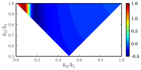
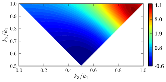
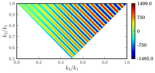
Figure 1: Density plots of the scalar non-Gaussianity parameter $f_{{}_{\rm NL}}$, plotted as function of $k_{3}/k_{1}$ and $k_{2}/k_{1}$, with fixed values of $k_{1}$, in the three models of our interest, viz. punctuated inflation (on top), quadratic potential with a step (in the middle) and axion monodromy model (at the bottom). We have chosen the wavenumber $k_{1}$ to be $10^{-3}\;{\rm Mpc}^{-1}$ in the case of punctuated inflation, while we have set it to be $2\times 10^{-3}\;{\rm Mpc}^{-1}$ for the other two models. We find that, when the features are localized, as in the cases of punctuated inflation and the quadratic potential with a step, the structure of $f_{{}_{\rm NL}}$ varies considerably with the choice of $k_{1}$. However, in the case of the axion monodromy model, wherein there arises continued oscillations, the shape of $f_{{}_{\rm NL}}$ is more or less independent of the choice of $k_{1}$.

non-Gaussianity parameter $f_{{}_{\rm NL}}$, for an arbitrary triangular configuration of the wavenumbers. Usually, the scalar bi-spectrum and the parameter $f_{{}_{\rm NL}}$ are illustrated as density plots, plotted as a function of the ratios $k_{3}/k_{1}$ and $k_{2}/k_{1}$, for a fixed value of $k_{1}$ (in this context, see, for instance, Ref. [38]). While the actual value of $k_{1}$ will not play a significant role in simple slow roll scenarios, the structure of the bi-spectrum revealed in such density plots will depend on choice of $k_{1}$ in models which lead to features. In Fig. 1, we have plotted the scalar non-Gaussianity parameter arising in the three inflationary models of our interest, for suitable values of the quantity $k_{1}$. We find that, in the cases of punctuated inflation and the quadratic potential with a step, since the features are localized over a small range of scales, the structure of the plot changes to a certain extent with the choice of $k_{1}$. However, in the case of axion monodromy model, because of the reason that the oscillations extend over a wide range of scales, the choice of $k_{1}$ does not alter the structure of the plots significantly.

In Fig. 2, we have attempted to capture the complete structure and shape of the bi-spectrum using a three-dimensional contour plot. We have made use of Mayavi and Python to create the three-dimensional plot [62].

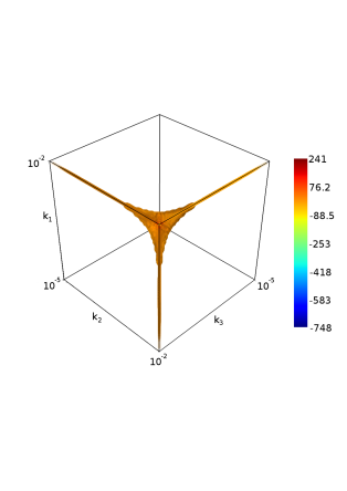
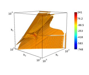
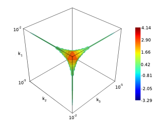
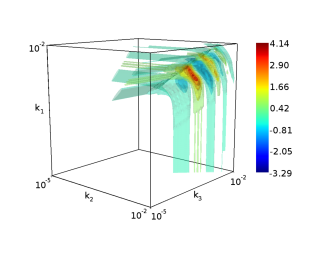
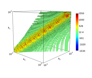
Figure 2: Three-dimensional contour plots of the parameter $f_{{}_{\rm NL}}$, plotted against the three wavenumbers $k_{1}$, $k_{2}$ and $k_{3}$ in the three models of interest, organized in the same order as in the last figure. We have shown two different projections of the plots in the figure. The projections in the left column clearly indicate the symmetry along the three different axes, as is expected in an isotropic background. The figures on the right column illustrate the fact that the allowed domain of wavenumbers are confined to a ‘tetrapyd’ and that the bi-spectrum peaks in the equilateral limit, i.e. along the line $k_{1}=k_{2}=k_{3}$.

We have plotted the parameter $f_{{}_{\rm NL}}$ for a wide range of the wavenumbers $k_{1}$, $k_{2}$ and $k_{3}$, over the allowed domain wherein the corresponding wavevectors satisfy the triangularity condition. It is known that the triangularity condition restricts the wavenumbers to a ‘tetrapyd’, as is evident from the figure. In the figure, we have presented two projections of the three-dimensional plot. One of the views clearly shows the fact that the bi-spectrum is symmetric along the three axes, as is expected in an isotropic background. The second illustrates the fact the non-Gaussianity parameter peaks in the equilateral limit, i.e. when $k_{1}=k_{2}=k_{3}$.

4.2 $f_{{}_{\rm NL}}$ in the squeezed limit

Let us now turn to examine the consistency relation in the three models of our interest. Towards this end, we have made use of BINGO to evaluate the non-Gaussianity parameter $f_{{}_{\rm NL}}$ in the squeezed limit, using the Maldacena formalism. As we had pointed out, BINGO can be made use of to evaluate the power spectrum as well. Using the expression (2.6) and the scalar power spectrum, we arrive at the scalar spectral index $n_{{}_{\rm S}}$, which we then utilize to verify the consistency condition $f_{{}_{\rm NL}}(k)=5\,\left[n_{{}_{\rm S}}(k)-1\right]/12$. Before we go on to illustrate the results for the three models that we are focusing on, a couple of points concerning the squeezed limit needs to be made. We should stress that we take the wavenumber of the squeezed mode to be smallest wavenumber that is numerically tenable in the sense that the mode is sufficiently inside the Hubble radius at a time close to when the integration of the background begins. Moreover, it should be noted that, since the squeezed mode has a finite and non-zero wavenumber, in the squeezed limit of our interest, the numerically evaluated bi-spectrum is expected to be more accurate at larger wavenumbers than the smaller ones. In Fig. 3, we have plotted the quantity $f_{{}_{\rm NL}}$ obtained from the Maldacena formalism as well as the quantity arrived at from the consistency relation. It is clear that the two quantities match very well (they match at the level of a few percent) thus confirming the validity of consistency relation even in scenarios displaying highly non-trivial dynamics.

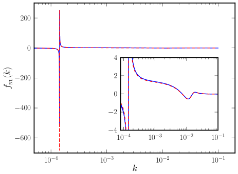
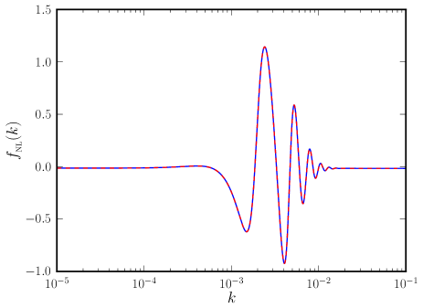
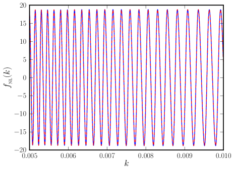
Figure 3: The behavior of the non-Gaussianity parameter $f_{{}_{\rm NL}}$ in the squeezed limit has been plotted as a function of $k$ for the three models, organized as in the previous two figures. The blue curve represents the $f_{{}_{\rm NL}}$ calculated using Maldacena formalism, while the red dashed line corresponds to the same quantity arrived at from the consistency relation. The excellent match between the two curves indicate that the consistency relation is valid even in non-trivial scenarios involving brief departures from inflation.

5 Discussion

At the level of the three-point function, the consistency condition relates the scalar bi-spectrum to the power spectrum in the squeezed limit wherein the wavelength of one of the three modes is much longer than the other two. As we had discussed, the consistency condition applies to any situation wherein the amplitude of the long wavelength mode freezes. Since the amplitude of the curvature perturbation settles down to a constant value on super-Hubble scales in most single field models of inflation, the consistency relation is expected to be valid in such models. It is easy to analytically establish the consistency relation in slow roll scenarios. In contrast, one needs to often resort to numerical methods to analyze situations involving departures from slow roll. In this work, we had examined the validity of the consistency condition, analytically as well as numerically, in a class of models permitting deviations from slow roll. We find that the condition is indeed satisfied even in situations consisting of strong departures from slow roll, such as the punctuated inflationary scenario.

With the emergence of increasingly precise cosmological data, it has been recognized that correlation functions beyond the power spectrum can act as powerful probes of the early universe. However, as we had discussed in the introductory section, despite the relatively strong bounds that have been arrived at on the scalar non-Gaussianity parameter $f_{{}_{\rm NL}}$, there exist a wide range of models that remain consistent with the data. The consistency relations can obviously play an important role to alleviate the situation. For instance, if the consistency relations can be observationally confirmed, it can rule out many multi-field models of inflation and even, possibly, alternate scenarios such as the bouncing models (in this context, see, for instance, Refs. [63, 64] and references therein). It seems worthwhile to closely investigate the conditions under which the consistency relation holds in, say, two-field models (see, for example, Ref. [65]) and, in particular, examine in some detail the role the iso-curvature perturbations may play in this regard. We are currently studying such issues.

References

- [1] A. A. Starobinsky, JETP Lett. 30, 682 (1979); V. F. Mukhanov and G. V. Chibisov, JETP Lett. 33, 532 (1981); S. W. Hawking, Phys. Lett. B 115, 295 (1982); A. A. Starobinsky, Phys. Lett. B 117, 175 (1982); A. Guth and S.-Y. Pi, Phys. Rev. Lett. 49, 1110 (1982); A. A. Starobinsky, Astron. Lett. 9, 302 (1983); V. N. Lukash, Sov. Phys. JETP 52, 807 (1980); D. H. Lyth, Phys. Rev. D 31, 1792 (1985).
- [2] E. W. Kolb and M. S. Turner, The Early Universe (Addison-Wesley, Redwood City, California, 1990); S. Dodelson, Modern Cosmology (Academic Press, San Diego, U.S.A., 2003); V. F. Mukhanov, Physical Foundations of Cosmology (Cambridge University Press, Cambridge, England, 2005); S. Weinberg, Cosmology (Oxford University Press, Oxford, England, 2008); R. Durrer, The Cosmic Microwave Background (Cambridge University Press, Cambridge, England, 2008); D. H. Lyth and A. R. Liddle, The Primordial Density Perturbation (Cambridge University Press, Cambridge, England, 2009); P. Peter and J-P. Uzan, Primordial Cosmology (Oxford University Press, Oxford, England, 2009); H. Mo, F. v. d. Bosch and S. White, Galaxy Formation and Evolution (Cambridge University Press, Cambridge, England, 2010).
- [3] H. Kodama and M. Sasaki, Prog. Theor. Phys. Suppl. 78, 1 (1984); V. F. Mukhanov, H. A. Feldman and R. H. Brandenberger, Phys. Rep. 215, 203 (1992); J. E. Lidsey, A. Liddle, E. W. Kolb, E. J. Copeland, T. Barreiro and M. Abney, Rev. Mod. Phys. 69, 373 (1997); A. Riotto, arXiv:hep-ph/0210162; W. H. Kinney, astro-ph/0301448; J. Martin, Lect. Notes Phys. 738, 193 (2008); J. Martin, Lect. Notes Phys. 669, 199 (2005); J. Martin, Braz. J. Phys. 34, 1307 (2004); B. Bassett, S. Tsujikawa and D. Wands, Rev. Mod. Phys. 78, 537 (2006); W. H. Kinney, arXiv:0902.1529 [astro-ph.CO]; L. Sriramkumar, Curr. Sci. 97, 868 (2009); D. Baumann, arXiv:0907.5424v1 [hep-th].
- [4] C. L. Bennet et al., Astrophys. J. Suppl. 436, 423 (1994); E. L. Wright et al., Astrophys. J. Suppl. 436, 443 (1994); K. M. Gorski, Astrophys. J. Suppl. 430, L85 (1994); K. M. Gorski et al., Astrophys. J. Suppl. 430, L89 (1994);
- [5] J. Dunkley et al., Astrophys. J. Suppl. 180, 306 (2009); E. Komatsu et al., Astrophys. J. Suppl. 180, 330 (2009).
- [6] D. Larson et al., Astrophys. J. Suppl. 192, 16 (2011); E. Komatsu et al., Astrophys. J. Suppl. 192, 18 (2011).
- [7] C. L. Bennett et al., Astrophys. J. Suppl. 208, 20 (2013); G. Hinshaw et al., Astrophys. J. Suppl. 208, 19 (2013).
- [8] P. A. R. Ade et al., arXiv:1303.5075 [astro-ph.CO].
- [9] P. A. R. Ade et al., arXiv:1303.5076 [astro-ph.CO].
- [10] P. A. R. Ade et al., arXiv:1303.5082 [astro-ph.CO].
- [11] P. A. R. Ade et al., arXiv:1403.4302 [astro-ph.CO].
- [12] P. A. R. Ade et al., Phys. Rev. Lett. 112, 241101 (2014).
- [13] J. Martin, C. Ringeval and V. Vennin, arXiv: 1303.3787 [astro-ph.CO].
- [14] J. Martin, C. Ringeval, R. Trotta and V. Vennin, JCAP 1403, 039 (2014); arXiv:1405.7272 [astro-ph.CO].
- [15] J. Martin, C. Ringeval and V. Vennin, arXiv:1407.4034 [astro-ph.CO].
- [16] E. Komatsu and D. N. Spergel, Phys. Rev. D 63, 063002 (2001).
- [17] P. A. R. Ade et al., arXiv:1303.5084 [astro-ph.CO].
- [18] J. Maldacena, JHEP 0305, 013 (2003).
- [19] P. Creminelli and M. Zaldarriaga, JCAP 0410, 006 (2004).
- [20] C. Cheung, A. L. Flitzpatrick, J. Kaplan and L. Senatore, JCAP 0802, 021 (2008); S. Renaux-Petel, JCAP 1010, 020 (2010); J. Ganc and E. Komatsu, JCAP 1012, 009 (2010); P. Creminelli, G. D’Amico, M. Musso and J. Norena, JCAP 1111, 038 (2011); D. Chialva, JCAP 1210, 037 (2012); K. Schalm, G. Shiu and T. van der Aalst, JCAP 1303, 005 (2013); E. Pajer, F. Schmidt and M. Zaldarriaga, Phys. Rev. D 88, 083502 (2013).
- [21] L. Senatore and M. Zaldarriaga, JCAP 1208, 001 (2012); P. Creminelli, J. Norena and M. Simonovoc, JCAP 1207, 052 (2012); P. Creminelli, A. Perko, L. Senatore, M. Simonovic and G. Trevisan, JCAP 1311, 015 (2013); L. Berezhiani and J. Khoury, JCAP 1402, 003 (2014); L. Berezhiani, J. Khoury and J. Wang, arXiv:1401.7991 [hep-th]; H. Collins, R. Holman and T. Vardanyan, arXiv:1405.0017 [hep-th].
- [22] J. Maldacena and G. L. Pimentel, JHEP 1109, 045 (2011); X. Gao, T. Kobayashi, M. Yamaguchi and J. Yokoyama, Phys. Rev. Lett. 107, 211301 (2011).
- [23] X. Gao, T. Kobayashi, M. Shiraishi, M. Yamaguchi, J. Yokoyama and S. Yokoyama, arXiv:1207.0588 [astro-ph.CO].
- [24] D. Jeong and M. Kamionkowski, Phys. Rev. Lett. 108, 251301 (2012); L. Dai, D. Jeong and M. Kamionkowski, Phys. Rev. D 87, 103006 (2013); Phys. Rev. D 88, 043507 (2013).
- [25] V. Sreenath, R. Tibrewala and L. Sriramkumar, JCAP 1312, 037 (2013).
- [26] S. Kundu, arXiv:1311.1575 [astro-ph.CO].
- [27] V. Sreenath and L. Sriramkumar, arXiv:1406.1609 [astro-ph.CO].
- [28] S. M. Leach and A. R. Liddle, Phys. Rev. D 63, 043508 (2001); S. M. Leach, M. Sasaki, D. Wands and A. R. Liddle, ibid. 64, 023512 (2001); R. K. Jain, P. Chingangbam and L. Sriramkumar, JCAP 0710, 003 (2007).
- [29] R. H. Ribeiro, JCAP 1205, 037 (2012); J. Martin, H. Motohashi and T. Suyama, Phys. Rev. D 87, 023514 (2013); M. G. Jackson and G. Shiu, Phys. Rev. D 88, 123511 (2013); R. Flauger, D. Green, R. A. Porto, JCAP 1308, 032 (2013); J. Gong, K. Schalm and G. Shiu, Phys. Rev. D 89, 063540 (2014).
- [30] P. Adshead, W. Hu, C. Dvorkin and H. V. Peiris, Phys. Rev. D 84, 043519 (2011); A. Achucarro, J-O. Gong, G. A. Palma and S. P. Patil, Phys. Rev. D 87, 121301 (2013).
- [31] M. H. Namjoo, H. Firouzjahi and M. Sasaki, Europhys. Lett. 101, 39001 (2013); X. Chen, H. Firouzjahi, M. Namjoo and M. Sasaki, Europhys. Lett. 102, 59001 (2013).
- [32] J. Ganc, Phys. Rev. D 84, 063514 (2011); I. Agullo and L. Parker, Phys. Rev. D 83, 063526 (2011); Gen. Rel. Grav. 43, 10 (2011).
- [33] T. Bunch and P. C. W. Davies, Proc. Roy. Soc. Lond. A 360, 117 (1978).
- [34] D. Seery and J. E. Lidsey, JCAP 0506, 003 (2005); X. Chen, Phys. Rev. D 72, 123518 (2005); X. Chen, M.-x. Huang, S. Kachru and G. Shiu, JCAP 0701, 002 (2007); D. Langlois, S. Renaux-Petel, D. A. Steer and T. Tanaka, Phys. Rev. Lett. 101, 061301 (2008); Phys. Rev. D 78, 063523 (2008).
- [35] X. Chen, Adv. Astron. 2010, 638979 (2010); Y. Wang, arXiv:1303.1523 [hep-th].
- [36] J. Martin and L. Sriramkumar, JCAP 1201, 008 (2012).
- [37] D. K. Hazra, J. Martin and L. Sriramkumar, Phys. Rev. D 86, 063523 (2012).
- [38] D. K. Hazra, L. Sriramkumar and J. Martin, JCAP 05, 026 (2013).
- [39] L. F. Abbott and M. B. Wise, Nucl. Phys. B 244, 541 (1984); D. H. Lyth and E. D. Stewart, Phys. Lett. B 274, 168 (1992); J. Martin and D. J. Schwarz, Phys. Rev. D 57, 3302 (1998); L. Sriramkumar and T. Padmanabhan, Phys. Rev. D 71, 103512 (2005).
- [40] I. S. Gradshteyn and I. M. Ryzhik, Table of Integrals, Series and Products, Seventh Edition (Acedemic Press, New York, 2007).
- [41] A. A. Starobinsky, Sov. Phys. JETP Lett. 55, 489 (1992).
- [42] F. Arroja, A. E. Romano and M. Sasaki, Phys. Rev. D 84, 123503 (2011); F. Arroja and M. Sasaki, JCAP 1208, 012 (2012).
- [43] J. Martin, L. Sriramkumar and D. K. Hazra, arXiv:1404.6093 [astro-ph.CO]
- [44] E. D. Stewart, Phys. Rev. D 65, 103508 (2002); J. Choe, J-O. Gong and E. D. Stewart, JCAP 0407, 012 (2004); J-O. Gong, JCAP 0507, 015 (2005).
- [45] R. K. Jain, P. Chingangbam, J.-O. Gong, L. Sriramkumar and T. Souradeep, JCAP 0901, 009 (2009); R. K. Jain, P. Chingangbam, L. Sriramkumar and T. Souradeep, Phys. Rev. D 82, 023509 (2010).
- [46] L. Lello, D. Boyanovsky and R. Holman, arXiv:1307.4066 [astro-ph.CO]; M. Cicoli, S. Downes and B. Dutta, arXiv:1309.3412 [hep-th]; F. G. Pedro and A. Westphal, arXiv:1309.3413 [hep-th].
- [47] J. A. Adams, B. Cresswell and R. Easther, Phys. Rev. D 64, 123514 (2001); L. Covi, J. Hamann, A. Melchiorri, A. Slosar and I. Sorbera, Phys. Rev. D 74, 083509 (2006); J. Hamann, L. Covi, A. Melchiorri and A. Slosar, Phys. Rev. D 76, 023503 (2007); M. J. Mortonson, M. Joy, V. Sahni and A. A. Starobinsky, Phys. Rev. D 77, 023514 (2008); M. Joy, A. Shafieloo, V. Sahni and A. A. Starobinsky, JCAP 0906, 028 (2009); C. Dvorkin, H. V. Peiris and W. Hu, Phys. Rev. D 79, 103519 (2009); C. Dvorkin and W. Hu, Phys. Rev. D 81, 023518 (2010); W. Hu, arXiv:1104.4500v1 [astro-ph.CO].
- [48] A. Ashoorioon and A. Krause, arXiv:hep-th/0607001; A. Ashoorioon, A. Krause and K. Turzynski, JCAP 0902, 014 (2009).
- [49] D. K. Hazra, M. Aich, R. K. Jain, L. Sriramkumar and T. Souradeep, JCAP 1010, 008 (2010).
- [50] M. Benetti, M. Lattanzi, E. Calabrese and A. Melchiorri, Phys. Rev. D 84, 063509 (2011); M. Benetti, arXiv:1308.6406 [astro-ph.CO].
- [51] J. Martin and C. Ringeval, Phys. Rev. D 69, 083515 (2004); Phys. Rev. D 69, 127303 (2004); JCAP 0501, 007 (2005); M. Zarei, Phys. Rev. D 78, 123502 (2008).
- [52] C. Pahud, M. Kamionkowski and A. R. Liddle, Phys. Rev. D 79, 083503 (2009).
- [53] R. Flauger, L. McAllister, E. Pajer, A. Westphal and G. Xu, JCAP 1006, 009 (2010).
- [54] M. Aich, D. K. Hazra, L. Sriramkumar and T. Souradeep, Phys. Rev. D 87, 083526 (2013).
- [55] H. Peiris, R. Easther and R. Flauger, arXiv:1303.2616 [astro-ph.CO]; R. Easther and R. Flauger, arXiv:1308.3736 [astro-ph.CO].
- [56] P. D. Meerburg, D. N. Spergel and B. D. Wandelt, arXiv:1308.3704 [astro-ph.CO]; P. D. Meerburg and D. N. Spergel, arXiv:1308.3705 [astro-ph.CO]; P. D. Meerburg, arXiv:1406.3243 [astro-ph.CO].
- [57] J. Martin, C. Ringeval and R. Trotta, Phys. Rev. D 83, 063524 (2011); M. J. Mortonson, H. V. Peiris and R. Easther, Phys. Rev. D 83, 043505 (2011); R. Easther and H. Peiris, Phys. Rev. D 85, 103533 (2012); J. Norena, C. Wagner, L. Verde, H. V. Peiris and R. Easther, Phys. Rev. D 86, 023505 (2012).
- [58] D. K. Hazra, A. Shafieloo and T. Souradeep, JCAP 1307, 031 (2013); arXiv:1406.4827 [astro-ph.CO]; P. Hunt and S. Sarkar, arXiv:1308.2317 [astro-ph.CO].
- [59] D. S. Salopek, J. R. Bond and J. M. Bardeen, Phys. Rev. D 40, 1753 (1989); C. Ringeval, Lect. Notes Phys. 738, 243 (2008).
- [60] X. Chen, R. Easther and E. A. Lim, JCAP 0706, 023 (2007); JCAP 0804, 010 (2008).
- [61] S. Hotchkiss and S. Sarkar, JCAP 1005, 024 (2010); S. Hannestad, T. Haugbolle, P. R. Jarnhus and M. S. Sloth, JCAP 1006, 001 (2010); R. Flauger and E. Pajer, JCAP 1101, 017 (2011); P. Adshead, W. Hu, C. Dvorkin and H. V. Peiris, Phys. Rev. D 84, 043519 (2011); X. Chen, JCAP 1201, 038 (2012); P. Adshead, W. Hu and V. Miranda, Phys. Rev. D 88, 023507 (2013).
- [62] P. Ramachandran and G. Varoquaux, IEEE Computing in Science and Engineering 13, 40 (2011)
- [63] D. Battefeld and P. Peter, arXiv:1406.2790 [astro-ph.CO].
- [64] X. Gao, M. Lilley and P. Peter, arXiv:1406.4119 [gr-qc].
- [65] V. Assassi, D. Baumann and D. Green, JCAP 1211, 047 (2012).