A coupled cohesive zone model for transient analysis of thermoelastic interface debonding

Abstract

A coupled cohesive zone model based on an analogy between fracture and contact mechanics is proposed to investigate debonding phenomena at imperfect interfaces due to thermomechanical loading and thermal fields in bodies with cohesive cracks. Traction-displacement and heat flux-temperature relations are theoretically derived and numerically implemented in the finite element method. In the proposed formulation, the interface conductivity is a function of the normal gap, generalizing the Kapitza constant resistance model to partial decohesion effects. The case of a centered interface in a bimaterial component subjected to thermal loads is used as a test problem. The analysis focuses on the time evolution of the displacement and temperature fields during the transient regime before debonding, an issue not yet investigated in the literature. The solution of the nonlinear numerical problem is gained via an implicit scheme both in space and in time. The proposed model is finally applied to a case study in photovoltaics where the evolution of the thermoelastic fields inside a defective solar cell is predicted.
Note: this is the author’s version of a work that was accepted for publication in Computational Mechanics. Changes resulting from the publishing process, such as editing, structural formatting, and other quality control mechanisms may not be reflected in this document. A definitive version was published in Computational Mechanics, Vol. 53, October 2013, 845-857, DOI:10.1007/s00466-013-0934-8

and

1 Introduction

The problem of stress and heat transfer across an interface between elastically dissimilar materials is relevant in engineering applications. If the bodies are initially separated and then pressed into contact, surface roughness is a limiting factor to achieve the conductivity of the bulk. A strategy to take into account the effect of roughness in finite element computations has been proposed in [1] by implementing a modified penalty formulation with a contact law based on a thermo-plastic microscopic contact model [2] in the node-to-segment contact geometry. In case of geometrically linear problems where finite displacements in the contact region do not take place, a simplification of the rigorous formulation in [1] by using two-node contact elements has been proposed in [3]. Since the adopted physical law contains dependencies from variables whose values change during the analysis, an elegant consistent linearization of the constitutive equations was proposed for the nonlinear iterative procedure.

Another set of problems where stress and heat transfers across an interface have to be computed is when initially fully bonded bodies progressively debond in tension due to thermomechanical deformations. The constitutive relations have to characterize the progressive reduction of stress transfer and heat flux due to increasing interfacial damage. In the framework on nonlinear fracture mechanics, a thermomechanical cohesive zone model for bridged delamination cracks in laminated composites has been proposed in [4, 5]. This thermomechanical cohesive zone model formulation has been revisited in [6] and an application to polycrystalline materials under Mixed Mode deformation was presented. In building physics, the interface conductivity of bonded joints is an important property for the assessment of reliability of insulation by using the well-known Glaser diagram. In this field, a coupled problem between the thermal field and the moisture diffusion can be of interest to avoid humidity condensation inside insulated walls. In certain cases, coupling with the elastic field has to be considered to predict the occurrence of plaster decohesion. In this class of problems, interface cracks require specific constitutive models to depict decohesion, moisture and heat transfer. This led in [7] to a hygro-thermomechanical cohesive zone model specific for modelling the phenomena of conduction in porous media. Other computational work in this area regards hygro-mechanical problems at interfaces [8, 9, 10], a coupled problem which shares some features with thermomechanics.

In the aforementioned contributions related to the thermomechanical behaviour of interfaces, either in compression or in tension, the heat flux is considered to be dependent on the interface closure (for contact mechanics) or opening (for fracture mechanics). However, there are several applications in the field on nanocomposites [11] where a constant interface conductivity is used. This approach, called Kapitza model, can be regarded as a constant spring in the framework of nonlinear spring elements. In spite of its simplicity, this approach permits to simulate a range of interface behaviors from highly conductive to perfectly insulated, depending on the value of the Kapitza resistance. Examples restricted to the thermal problem without coupling with the mechanical one are discussed in [12, 13]. Although the mathematical formulation is simpler due to the lack of coupling between the elastic and the thermal variables in the interface constitutive relation, the Kapitza coefficient is hard to be identified unless the interface is a well defined intermediate material region with a given thickness.

In this study, a novel thermomechanical cohesive zone model is proposed for the study of decohesion at material interfaces due to thermal and mechanical loads. As compared to the state-of-the-art literature on this matter, several novelties are presented. The interface contact conductivity relation and its coupling with the crack opening is derived by exploiting an analogy with contact mechanics of rough surfaces, using the recent results established in [14, 15]. This leads to an interface constitutive relation with a limited number of free parameters of physical meaning that can be identified from the quantitative analysis of roughness of cracked interfaces. Moreover, the thermal analysis focuses on the transient regime, obtained according to a solution strategy implicit both in space and in time. Previous studies were limited to the analysis of the steady state solution. A comparison between the proposed approach with a fully coupled heat-conduction model dependent on the displacement field and the uncoupled formulation based on the Kapitza model is proposed. Contrary to the contact problem in [3], where the coupling term was found to be of low importance for the considered example, in the present case the unsymmetrical coupled term of the stiffness matrix is relevant due to the nonlinearity of the thermoelastic cohesive zone model. Finally, an application to photovoltaics is proposed to show the effect of cohesive cracks on the thermoelastic fields inside a defective solar cell.

2 Formulation of the thermomechanical problem with cohesive interfaces

The partial differential equations governing the mechanical equilibrium in a solid body (Fig.1) with volume $V$ and surface $S$ written in vectorial form are:

$$\nabla^{\mathrm{T}}\textbf{S}\textbf{+f=0},$$ (1)

where $\nabla$ is the gradient vector, S is the Cauchy stress tensor and f is the vector of body forces. By introducing the displacement vector w and the stress vector $\sigma$, the weak form corresponding to Eq. (1), i.e. the principle of virtual works, writes:

$$\begin{array}[]{ll}&\displaystyle{\int_{V}\textbf{S}:\nabla(\delta\textbf{w})\mathrm{d}V=}\\ &\displaystyle{\int_{V}\textbf{f}^{\mathrm{T}}\delta\textbf{w}\mathrm{d}V+\int_{S}\overline{\sigma}^{\mathrm{T}}\delta\textbf{w}\mathrm{d}S+\int_{S_{int}}\sigma^{\mathrm{T}}\delta(\Delta\textbf{w})\mathrm{d}S,}\end{array}$$ (2)

where $\overline{\sigma}$ is the vector of prescribed tractions on the boundary, while $S_{int}$ represents the internal surface. Note that in Eq. (2) the notation

$$\textbf{S}:\nabla(\delta\textbf{w})=S_{ij}\dfrac{\partial\delta w_{i}}{\partial x_{j}}$$

has been adopted.

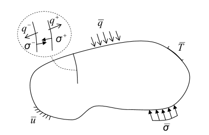
Figure 1: Solid body with a cohesive interface.

The partial differential equation governing the transient heat conduction problem in the solid reads:

$$-\nabla^{\mathrm{T}}\textbf{q}+Q=d_{m}\,c\,\dot{T},$$ (3)

where q is the heat flux vector, $Q$ is the heat generation per unit volume per unit time, $d_{m}$ is the material density, $c$ is the specific heat and $T$ is the temperature. By means of Fourier’s law $\textbf{q}=-k\nabla T$, $k$ being the material conductivity, Eq.(3) can be rewritten as:

$$k\nabla^{2}T+Q=d_{m}\,c\,\dot{T}.$$ (4)

The weak form related to the heat conduction problem, i.e. the variational form of the energy balance, is then expressed as:

$$\begin{array}[]{ll}&\displaystyle{\int_{V}\textbf{q}^{\mathrm{T}}\nabla(\delta T)\mathrm{d}V=-\int_{V}k(\nabla T)^{\mathrm{T}}\nabla\delta T\mathrm{d}V=}\\ &\displaystyle{\int_{V}(d_{m}\,c\,\dot{T}-Q)\delta T\,\mathrm{d}V+\int_{S}\overline{q}\delta T\,\mathrm{d}S+\int_{S_{int}}q\delta(\Delta T)\,\mathrm{d}S.}\end{array}$$ (5)

where $\overline{q}$ represents the prescribed external heat flux per unit area, normal to the boundary.

The last terms in Eqs.(2) and (5) represent the contribution of the cohesive tractions and heat flux for the displacement jump, $\Delta\textbf{w}$, and temperature jump, $\Delta\textbf{T}$, across the interface.

3 Finite element discretization of thermoelastic cohesive interfaces

The coupled thermomechanical problem for the continuum can be discretized by using standard four-node quadrilateral finite elements (FE) with a mixed formulation. As regards the cohesive interfaces, a four-node linear interface element compatible with the elements used to discretize the continuum can be introduced, as sketched in Fig.2. As compared to the 2D formulation for mechanical problems [16, 17], each node has three generalized degrees of freedom in the global reference system instead of two: the horizontal displacement $u_{i}$, the vertical displacement $v_{i}$ and the temperature $T_{i}$. In 3D, four degrees of freedom for each node have to be specified. These generalized displacements can be collected in the element vector $\mathbf{u}$:

$$\mathbf{u}=\left(u_{1},v_{1},T_{1},u_{2},v_{2},T_{2},u_{3},v_{3},T_{3},u_{4},v_{4},T_{4}\right)^{T}.$$ (6)

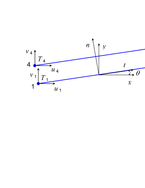
Figure 2: Bi-dimensional linear interface element.

A local reference system defined by the tangential vector $t$ and the normal vector $n$ to the interface element is introduced, see Fig.2. The origin $O$ of the local reference system is placed in the center of the element, which is in general rotated with respect to the global $x-$axis by an angle $\theta$. The generalized vector $\textbf{u}^{*}$ of the $i-$th node in the local coordinate system can be computed via a pre-multiplication by a rotation matrix, $\mathbf{u_{i}}^{*}=\mathbf{r}\mathbf{u_{i}}$, i.e.:

$$\left\{\begin{array}[]{c}u_{i}^{*}\\ v_{i}^{*}\\ T_{i}^{*}\end{array}\right\}=\left[\begin{array}[]{rrr}\cos\theta&\,\sin\theta&0\\ -\sin\theta&\,\cos\theta&0\\ 0&0&1\end{array}\right]\left\{\begin{array}[]{c}u_{i}\\ v_{i}\\ T_{i}\end{array}\right\}.$$ (7)

Therefore, the generalized displacement vector of the whole interface element in the local reference system, $\mathbf{u}^{*}$, can be related to $\mathbf{u}$ as follows:

$$\mathbf{u}^{*}=\mathbf{R}\mathbf{u},$$ (8)

where $\mathbf{R}$ is obtained by the collection of the individual rotation matrices $\mathbf{r}$:

$$\mathbf{R}=\left[\begin{array}[]{cccc}\mathbf{r}&0&0&0\\ 0&\mathbf{r}&0&0\\ 0&0&\mathbf{r}&0\\ 0&0&0&\mathbf{r}\end{array}\right].$$ (9)

The relative generalized displacement vector $\mathbf{\Delta u}^{*}=(u_{4}^{*}-u_{1}^{*},v_{4}^{*}-v_{1}^{*},T_{4}^{*}-T_{1}^{*},u_{3}^{*}-u_{2}^{*},v_{3}^{*}-v_{2}^{*},T_{3}^{*}-T_{2}^{*})^{\mathrm{T}}$ can now be computed as $\mathbf{\Delta u}^{*}=\mathbf{L}\mathbf{u}^{*}$, where the operator matrix $\mathbf{L}$ relates the displacement and temperature field components to the relative displacements and temperatures between the upper and the lower sides of the interface, $\Gamma^{+}$ and $\Gamma^{-}$:

$$\mathbf{L}=\left[\begin{array}[]{cccccccccccc}-1&0&0&0&0&0&0&0&0&+1&0&0\\ 0&-1&0&0&0&0&0&0&0&0&+1&0\\ 0&0&-1&0&0&0&0&0&0&0&0&+1\\ \ 0&0&0&-1&0&0&+1&0&0&0&0&0\\ 0&0&0&0&-1&0&0&+1&0&0&0&0\\ 0&0&0&0&0&-1&0&0&+1&0&0&0\\ \end{array}\right].$$ (10)

The vector of the tangential, normal and temperature gaps for a generic point along the interface element, $\mathbf{g}=(g_{\mathrm{t}},g_{\mathrm{n}},g_{T})^{{\mathrm{T}}}$, can be determined from $\mathbf{\Delta u}^{*}$ using standard interpolation functions, $\mathbf{g}=\mathbf{N}\mathbf{\Delta u}^{*}$, where $\mathbf{N}$ is given by

$$\mathbf{N}=\left[\begin{array}[]{cccccc}N_{1}&0&0&N_{2}&0&0\\ 0&N_{1}&0&0&N_{2}&0\\ 0&0&N_{1}&0&0&N_{2}\\ \end{array}\right].$$ (11)

In the present case, $N_{1}=(1-s)/2$ and $N_{2}=(1+s)/2$ are the linear shape functions. The $s$-coordinate ranges between $-1$ and $+1$, as for standard two-node isoparametric finite elements.

The vector $\mathbf{g}$ can therefore be related to the nodal generalized displacement vector as follows:

$$\mathbf{g}=\mathbf{N}\,\mathbf{L}\,\mathbf{R}\,\mathbf{u}=\mathbf{B}\,\mathbf{R}\,\mathbf{u}.$$ (12)

At this point, the constitutive relations for the interface, relating tractions and heat flux to displacement and temperature gaps, have to be introduced. For the sake of generality, we consider now a whatever nonlinear relation between those quantities. In the next section, a specific model will be introduced and the equations particularized to that case. The contribution to the weak form by the interface elements (Eqs. (2) and (5)) written in a compact way is:

$$\delta G_{int}=\int_{S_{int}}\delta\textbf{g}^{\mathrm{T}}\textbf{p}\,\mathrm{d}S,$$ (13)

where $\mathbf{p}=(\tau,\,\sigma,q)^{\mathrm{T}}$. Since the cohesive traction components $\sigma$ and $\tau$ and the heat flux $q$ may depend on quantities whose values vary during the simulation, a consistent linearization of the interface constitutive law has to be adopted for its use in the Newton-Raphson iterative method [17]:

$$\mathbf{p}=\mathbf{C}\,\mathbf{g}=\mathbf{C}\,\mathbf{B}\,\mathbf{R}\,\mathbf{u},$$ (14)

where the matrix $\mathbf{C}$ is the tangent constitutive matrix of the element:

$$\normalsize\mathbf{C}=\left[\begin{array}[]{ccc}\dfrac{\partial\tau}{\partial g_{\mathrm{t}}}&\dfrac{\partial\tau}{\partial g_{\mathrm{n}}}&0\\ \dfrac{\partial\sigma}{\partial g_{\mathrm{t}}}&\dfrac{\partial\sigma}{\partial g_{\mathrm{n}}}&0\\ \dfrac{\partial q}{\partial g_{\mathrm{t}}}&\dfrac{\partial q}{\partial g_{\mathrm{n}}}&\dfrac{\partial q}{\partial g_{T}}\\ \end{array}\right].$$ (15)

This matrix is in general not symmetric if the Mixed Mode cohesive zone model has different parameters for the Mode I and the Mode II traction components. Moreover, examining the coupling with the thermal field, two off-diagonal terms arise in the third row of Eq.(15) if the heat conduction constitutive relation is dependent on the opening and sliding displacements. As we will show in the sequel, these two terms are equal to zero in the Kapitza model, which allows for the use of uncoupled schemes and symmetric solvers.

By introducing Eqs.(12) and (14) into Eq. (13) we get:

$$\delta G_{int}=\delta\textbf{u}^{\mathrm{T}}\,\textbf{K}\,\textbf{u},$$ (16)

where

$$\textbf{K}=\textbf{R}^{\mathrm{T}}\int_{S_{int}}\textbf{B}^{\mathrm{T}}\textbf{C}\textbf{B}\,\mathrm{d}S\textbf{R}$$ (17)

is the tangent stiffness matrix of the element. In the following analysis, the integral in Eq. (17), as well as for the residual vector

$$\textbf{F}=\textbf{R}^{\mathrm{T}}\int_{S_{int}}\textbf{B}^{\mathrm{T}}\textbf{p}\,\mathrm{d}S,$$ (18)

will be computed using a two-point Gaussian quadrature scheme. The heat capacity matrix M is not considered for the interface element, since it is supposed to have a zero thickness. The transient regime will be solved according to the backward Euler method (implicit Euler method), which is a suitable scheme for the solution of the Fourier heat conduction equation.

This thermoelastic interface element has been implemented as a new user element in the finite element programme FEAP [18].

4 A thermomechanical cohesive zone model based on microscopical contact relations

The progressive separation of an interface due to the propagation of a crack can be modelled by the cohesive zone model (CZM) [19, 20]. According to the CZM, a relation between the normal (Mode I) and tangential (Mode II) cohesive tractions and the relative opening and sliding displacements experienced by the two opposite surfaces has to be defined. The various formulations for a pure Mode I problem are characterized by the peak cohesive traction, $\sigma_{\max}$, and the Mode I fracture energy, $G_{\mathrm{Ic}}$ , which is the area beneath the CZM curve. When the opening displacement $g_{\mathrm{n}}$ equals a critical value, $g_{\mathrm{nc}}$, a stress-free crack is created. Different shapes of the CZM, inspired by atomic potentials, have been proposed so far (see the qualitative sketch in Fig. 3): linear or bilinear softening CZMs are usually selected in case of brittle materials, whereas trapezoidal or bell-shape CZMs are used in case of ductile fracture. In some cases, linear and bilinear CZMs have an initial elastic branch with very high stiffness. This branch is necessary when interface elements are embedded from the very beginning of the numerical simulation into the finite element mesh along pre-defined interfaces.

Figure 3: Different shapes of the CZMs available in the literature.

If a suitable relationship between the thermal flux across the crack faces and the temperature jump is considered, the basic mechanical CZM formulation can be extended to thermoelastic problems leading to the so-called thermomechanical CZM. At this point, examining the state-of-the-art literature, the heat conduction equation was derived independently of the mechanical part of the CZM [6, 4, 5]. Therefore, additional parameters were introduced, whose identification is not trivial.

In case of an interface without fibers, an analogy with contact mechanics can be put forward to simplify the matter. During contact, a compressive pressure $p$ (negative valued) is applied to the rough surface and it ranges from zero (first point of contact corresponding to the tallest asperity) to the full contact pressure, $p_{\mathrm{c}}$ (see Fig. 4). In case of fracture, the process is basically reversed. The full contact regime can be regarded as an intact interface and a (positive) tensile traction, equal in modulus to $p_{\mathrm{c}}$, has to be applied to separate the two bodies and create a stress-free crack. The process of debonding progressively produces a rough surface which finally leads to the microscopically rough stress-free crack (from left to right in Fig. 4). Hence, the Mode I cohesive traction $\sigma$ which, by definition, opposes to crack opening, can be evaluated for any mean plane separation between the rough surfaces, $g_{\mathrm{n}}$, as the opposite of the applied contact pressure $p$ for the same separation.

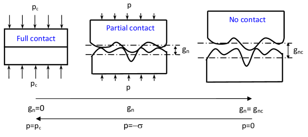
Figure 4: Cracked solid loaded by thermal and mechanical loads.

In case of elastic contact between two bodies with flat or rough boundaries, a theorem by Barber [14] demonstrates that the contact conductance is proportional to the normal contact stiffness. Hence, taking advantage of this result, it is possible to estimate the interface contact conductance directly from the solution of the normal contact problem, without the need of introducing additional ad hoc constitutive relations for the thermal response. In general, since the contact stiffness is dependent on the applied pressure, which is a function of the interface closure, the interface contact conductance will be dependent on the separation [15]. Dimensional analysis considerations and numerical results in [15] have demonstrated that the conductance-pressure relation is of power-law type, with an exponent close to unity. The linear case is admissible, and has been suggested by Greenwood and Williamson [21] with a microscopical contact model which assumes an exponential distribution of asperity heights. Independently, the linear relation between conductance and pressure has been proposed by Persson [22] in his contact model rigorously valid in the full contact regime.

Since we are considering a problem of decohesion, where the full contact regime is the starting point, we consider a linear conductance-pressure relation as by Greenwood and Williamson and by Persson and we propose an extension for the application to decohesion problems. The linear conductance-pressure relation implies an exponential decay of the cohesive traction w.r.t. the mean plane separation $g_{\mathrm{n}}$ between the rough surfaces. In the range $0\leq g_{n}<l_{0}$ (very low separations near the full contact regime), a linear regularization has to be introduced. With the use of intrinsic interface elements [23] already embedded in the FE mesh from the beginning of the simulation, an initial compliance of the CZM is necessary for the equilibrium with the continuum in the linear elastic regime. Although this regularization could be regarded as a pure numerical artefact, actually it can be related to the Young modulus and to the thickness of the interface region in case of adhesives [24, 27]. Finally, for separations $g_{\mathrm{n}}$ larger than $g_{\mathrm{nc}}$, a cut-off to the cohesive tractions corresponding to the formation of a stress-free crack is introduced. For real rough surfaces, this cut-off can be set at a distance equal to $3-4$ times the r.m.s. roughness $R$ of the crack profile.

Another modification is needed to consider the weakening effect of Mixed-Mode deformation, including the effect of the tangential sliding displacement $g_{\mathrm{t}}$ in the formulation. This can be done by adding a multiplicative term dependent on $g_{\mathrm{t}}$ and with the same form as for $g_{\mathrm{n}}$. According to these modeling assumptions, the resulting expression for the normal cohesive traction is the following:

$$\begin{array}[]{c}\sigma\end{array}\normalsize=\left\{\begin{array}[]{lrl}\sigma_{\max}\,\mathrm{exp}\left(\dfrac{-l_{0}-|g_{\mathrm{t}}|}{R}\right)\dfrac{g_{\mathrm{n}}}{l_{0}},&\mathrm{if}&\quad 0\leq\dfrac{g_{\mathrm{n}}}{R}<\dfrac{l_{0}}{R}\\ \sigma_{\max}\,\mathrm{exp}\left(\dfrac{-g_{\mathrm{n}}-|g_{\mathrm{t}}|}{R}\right),&\mathrm{if}&\quad\dfrac{l_{0}}{R}\leq\dfrac{g_{\mathrm{n}}}{R}<\dfrac{g_{\mathrm{nc}}}{R}\\ 0,&\mathrm{if}&\quad\dfrac{g_{\mathrm{n}}}{R}\geq\dfrac{g_{\mathrm{nc}}}{R}\\ \end{array}\right.$$ (19)

A similar relation can be proposed for the tangential cohesive tractions:

$$\begin{array}[]{c}\tau\end{array}\normalsize=\left\{\begin{array}[]{lrl}\tau_{\max}\,\mathrm{exp}\left(\dfrac{-l_{0}-g_{\mathrm{t}}}{R}\right)\dfrac{g_{\mathrm{t}}}{l_{0}},&\mathrm{if}&\quad 0\leq\dfrac{g_{\mathrm{t}}}{R}<\dfrac{l_{0}}{R}\\ \tau_{\max}\,\mathrm{sgn}(g_{\mathrm{t}})\,\mathrm{exp}\left(\dfrac{-g_{\mathrm{n}}-|g_{\mathrm{t}}|}{R}\right),&\mathrm{if}&\quad\dfrac{l_{0}}{R}\leq\dfrac{g_{\mathrm{t}}}{R}<\dfrac{g_{\mathrm{tc}}}{R}\\ 0,&\mathrm{if}&\quad\dfrac{g_{\mathrm{t}}}{R}\geq\dfrac{g_{\mathrm{tc}}}{R}\\ \end{array}\right.$$ (20)

where $\tau_{\max}$ and $g_{\mathrm{tc}}$ can be different from $\sigma_{\max}$ and $g_{\mathrm{nc}}$, respectively.

The interface contact conductance can now be determined via the first derivative of the normal pressure-separation relation w.r.t. $g_{\mathrm{n}}$ [14]:

$$\begin{array}[]{c}k_{\mathrm{int}}\end{array}\normalsize=\left\{\begin{array}[]{lrl}\dfrac{1}{\rho_{\mathrm{int}}},&\mathrm{if}&\quad 0\leq\dfrac{g_{\mathrm{n}}}{R}<\dfrac{l_{0}}{R}\\ \dfrac{2\sigma}{\rho_{\mathrm{int}}E_{\mathrm{int}}R},&\mathrm{if}&\quad\dfrac{l_{0}}{R}\leq\dfrac{g_{\mathrm{n}}}{R}<\dfrac{g_{\mathrm{nc}}}{R}\\ 0,&\mathrm{if}&\quad\dfrac{g_{\mathrm{n}}}{R}\geq\dfrac{g_{\mathrm{nc}}}{R},\\ \end{array}\right.$$ (21)

where a dependency on the normal contact pressure comes into play in the range $l_{0}\leq g_{\mathrm{n}}<g_{\mathrm{nc}}$. The resistivity $\rho_{\mathrm{int}}$ and the Young modulus $E_{\mathrm{int}}$ of the interface can be evaluated as $\rho_{\mathrm{int}}=\rho_{+}+\rho_{-}$ and $E_{\mathrm{int}}=[(1-\nu_{+}^{2})/E_{+}+(1-\nu_{-}^{2})/E_{-}]^{-1}$, where the subscripts $-$ and $+$ refer to the two materials separated by the interface and $\nu$ is the Poisson’s ratio. In the range $0\leq g_{n}<l_{0}$, a constant interface conductivity is selected. Since the maximum interface conductivity in contact problems can be attained for a small separation larger than zero, the parameter $l_{0}$ can be chosen according to this physical argument. In this range, with a constant $k_{\mathrm{int}}=1/\rho_{\mathrm{int}}$, the present approach is equivalent to the Kapitza model, where the coefficient $\rho_{\mathrm{int}}$ should be regarded as the Kapitza resistance.

As compared to previous thermomechanical CZMs, the main advantage of the proposed formulation relies in the fact that the thermal part of the CZM is simply derived from the normal stiffness and therefore it does not introduce additional independent model parameters. The complete thermomechanical CZM is therefore fully defined in terms of the maximum (peak) normal and shear tractions $\sigma_{\max}$ and $\tau_{\max}$, the critical gaps $g_{\mathrm{nc}}$ and $g_{\mathrm{tc}}$, the r.m.s. roughness $R$, an internal length $l_{0}$, the composite thermal resistance $\rho_{\mathrm{int}}$ and the composite Young’s modulus $E_{\mathrm{int}}$. Parameter identification should be carried out by choosing $\sigma_{\max}$ and $\tau_{\max}$ to capture the peak stresses deduced from tensile and shear tests on representative volume elements. The parameters $g_{\mathrm{nc}}$ and $g_{\mathrm{tc}}$ should be chosen to match the fracture toughness of the material. The additional parameter $l_{0}$ should be selected according to the physical compliance of the interface as proposed in [27]. The r.m.s. roughness $R$ can be quantified from a profilometric analysis of the crack path at failure. Finally, $\rho_{\mathrm{int}}$ has to be related to the resistivities of the bulk materials and it should be equal to the Kapitza resistance.

The normal cohesive traction (19) is plotted vs. $g_{\mathrm{n}}$ in Fig.5. It is interesting to note the similitude between the present formulation deduced according to contact mechanics considerations and the CZM by Xu and Needleman [25] and its subsequent generalizations [26]. In [25], the shape of the CZM is the result of the product between a linear function of the gap (dominating for small separations) and an exponential decay (prevailing for large separations), see the dashed curve in Fig.5(a). Although the shape of the Xu and Needleman CZM is not so different from the proposed expression and has the advantage of being defined by a single equation for the whole range of separations, if we attempt at estimating the interface contact conductance by differentiating it w.r.t. $g_{\mathrm{n}}$ we obtain an unphysical result. The interface contact conductance is negative at the beginning and it approaches that predicted by the present model only for very large separations, see Fig.5(b) obtained from the curves in Fig.5(a).

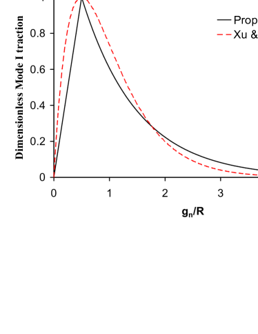
(a) Mode I CZM

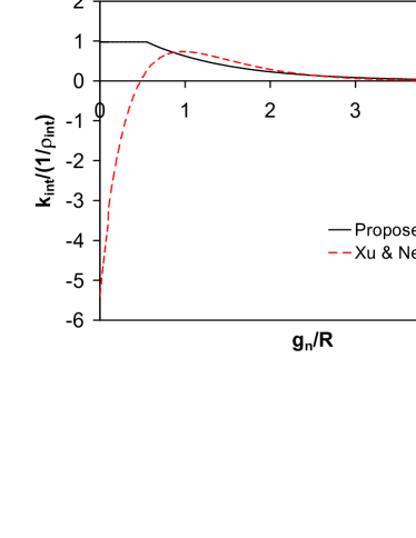
(b) Interface conductance

Figure 5: Comparison between the proposed CZM and that by Xu and Needleman [25] with matched parameters.

As a result of the proposed model, the interface conductance (21) does depend on the separation. The heat flux normal to the interface is given by $q=-k_{\mathrm{int}}\,g_{T}$. Its consistent linearization according to Eq.(15) provides the following terms for $0\leq g_{\mathrm{n}}/R<l_{0}/R$:

$$\dfrac{\partial q}{\partial g_{\mathrm{t}}} =0,$$ (22a)

$$\dfrac{\partial q}{\partial g_{\mathrm{n}}} =0,$$ (22b)

$$\dfrac{\partial q}{\partial g_{T}} =-\dfrac{1}{\rho_{\mathrm{int}}},$$ (22c)

and for $g_{\mathrm{n}}/R<g_{\mathrm{nc}}/R$:

$$\dfrac{\partial q}{\partial g_{\mathrm{t}}} =-\dfrac{2\,g_{T}}{\rho_{\mathrm{int}}\,E_{\mathrm{int}}\,R}\dfrac{\partial\sigma}{\partial g_{\mathrm{t}}},$$ (23a)

$$\dfrac{\partial q}{\partial g_{\mathrm{n}}} =-\dfrac{2\,g_{T}}{\rho_{\mathrm{int}}\,E_{\mathrm{int}}\,R}\dfrac{\partial\sigma}{\partial g_{\mathrm{n}}},$$ (23b)

$$\dfrac{\partial q}{\partial g_{T}} =-\dfrac{2\sigma}{\rho_{\mathrm{int}}\,E_{\mathrm{int}}\,R}.$$ (23c)

5 Numerical results

In this section we propose a simple example where we compare the present CZM predictions with those based on the Kapitza constant resistance model.

A bi-material composite of lateral side $L$, clamped at $x=0$ and at $x=L$ is considered (Fig. 6). A cohesive interface is placed at $x=L/2$. For the sake of simplicity, the bodies are assumed to have identical material properties.

An initial temperature $T_{i}$ is prescribed over the whole bodies and a temperature $T_{L}$ $(T_{L}<T_{i})$ is imposed along the right side ($x=L$, Fig. 6). We let the temperature vary inside the two bodies and along the other boundaries. Due to cooling of the right hand side, the material region $+$ will shrink more than the region $-$ and will progressively put in tension the interface until a possible debonding. This could be the case of a building wall with exposed surface on the right side.

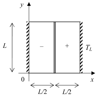
Figure 6: Square domain with a cohesive crack.

According to dimensional analysis arguments, for a given $y$, once the parameters $\nu$, $l_{0}$ and $R$ are prescribed, the temperature field $T$ throughout the body is a function of nine parameters:

$$T=T(x,L,T_{i},T_{L},t,D,E,g_{\mathrm{nc}},\sigma_{\max}),$$ (24)

where $D=k/(d_{m}c)$ is the thermal diffusion coefficient of the bulk. A dimensionless temperature $T^{*}=(T-T_{i})/(T_{i}-T_{L})$ can be introduced for the analysis of the results. A straightforward application of Buckingham theorem allows us reducing the dependency of $T^{*}$ on four parameters:

$$T^{*}=T^{*}\left(x^{*},t^{*},g_{\mathrm{nc}}^{*},\sigma_{\max}^{*}\right),$$ (25)

where:

$$x^{*}=\dfrac{x}{L},\;t^{*}=\dfrac{tD}{L^{2}},\;g_{\mathrm{nc}}^{*}=\dfrac{g_{\mathrm{nc}}}{L},\;\sigma_{\max}^{*}=\dfrac{\sigma_{\max}}{E}.$$

Notice that, when dealing with Kapitza’s model, also the interface dimensionless conductivity $k^{*}=k/k_{\mathrm{int}}$ will be introduced (Eq.(4)), for the sake of clarity.

In the next sections, numerical predictions will refer to $y/L=0.5$ by assuming plane stress conditions. The following parameters will be selected: $\nu=0.1$, $l_{0}/R=0.01$, $\sigma_{\max}^{*}=0.032$ and $g_{\mathrm{nc}}^{*}=0.05$.

5.1 Predictions according to Kapitza model

To provide a reference solution for quantifying the role of thermomechanical coupling in the interface constitutive relations, we first consider the simplified Kapitza model where the interface conductivity is a constant value. Hence, $k_{\mathrm{int}}=\mathrm{const}$ and this is the only non vanishing term entering the tangent constitutive matrix (15). The partial derivatives of the heat flux with respect to the normal and tangential gaps are zero. Therefore, the heat conduction equation and the equations of equilibrium become uncoupled in this case. This simplification allows for the implementation in FE codes where the mechanical and the thermal fields are solved separately. In particular, the thermal field should be solved first. Afterwards, the thermoelastic deformation has to be computed by solving the mechanical problem. The evolution of debonding will depend on the normal and tangential gaps at the interface and the stress field in the horizontal direction will be imposed by the mechanical part of the CZM constitutive relations.

Three cases are examined depending on the value of $k^{*}$, i.e., $k^{*}=0.001$, $k^{*}=1$ and $k^{*}=1000$. In Fig.7, $k^{*}=0.001$ and the interface is highly conductive. A parabolic profile of the temperature, with no discontinuities, is initially observed along $x^{*}$. At $t^{*}\simeq 125$, the interface debonds and the interface conductivity suddenly jumps from the value of $k^{*}$ to zero. Increasing time, the temperature of the two half bodies stabilize: the dimensionless temperature of the right part is progressively decreasing with time $t^{*}$ down to $-1$ .

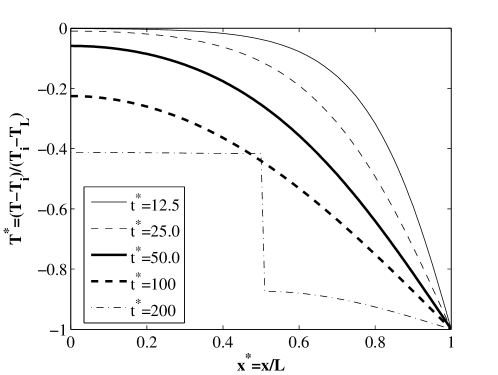
Figure 7: Kapitza’s model, $k^{*}=0.001$: dimensionless temperature field vs. dimensionless time.

For $k^{*}=1$ (see Fig.8), a temperature discontinuity is observed across the interface, since it is no longer highly conductive and it imposes a localized additional resistance to the system. Debonding takes place at $t^{*}\simeq 130$, similarly to the previous case.

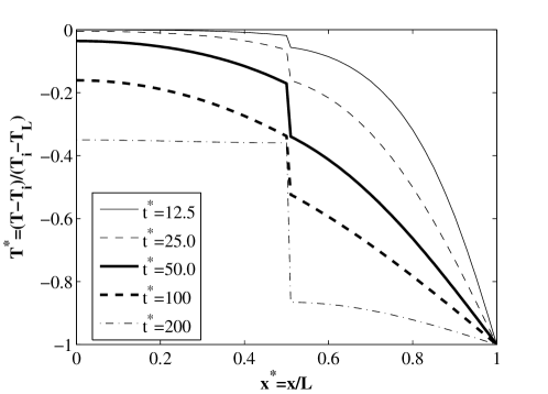
Figure 8: Kapitza’s model, $k^{*}=1$: dimensionless temperature field vs. dimensionless time.

For $k^{*}=1000$ (see Fig.9), the interface plays the role of an insulator and only the temperature of the right hand side varies with time, tending to the imposed value of $-1$. A negligible heat flux enters the left hand side, whose temperature remains nearly constant and equal to the initial one. For the chosen CZM parameters and the imposed dimensionless temperature jump, debonding does not take place in this case.

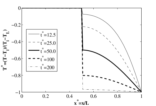
Figure 9: Kapitza’s model, $k^{*}=1000$: dimensionless temperature field vs. dimensionless time.

5.2 Proposed CZM predictions

The coupled thermomechanical CZM predictions are now presented. In this case, all the terms entering the tangent constitutive matrix (15) are different from zero and are considered. The solution is gained by solving for the thermal and the mechanical fields at the same time, since the crack opening influences the interface conductivity and therefore the solution of the thermal field. Moreover, an unsymmetrical solver is used due to the non symmetry of the interface element stiffness matrix.

The temperature and the horizontal displacement distributions predicted by the proposed CZM are shown in Fig.10 and 11, respectively, for different dimensionless times $t^{*}$.

Examining Fig.10, the temperature jump at the interface is initially an increasing function of $t^{*}$ due to the cooling of the right-hand side. Then the jump decreases: this process is relatively slow, due to the progressive opening of the cohesive crack which reduces the interface conductivity. Debonding takes place for $t^{*}\simeq 400$.

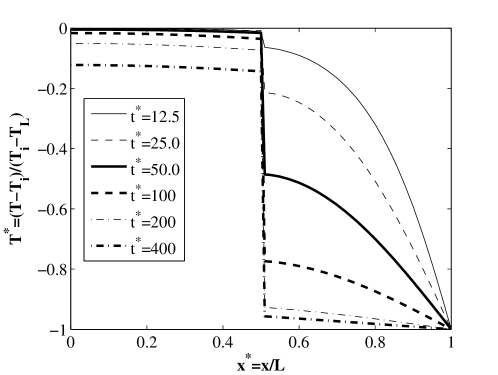
Figure 10: CZM predictions, dimensionless temperature field vs. dimensionless time.

Looking at the displacement field (Fig.11), two different stages are observed in the transient regime. In the range $0<t^{*}\leq 12.5$, the temperature of the right part decreases and the body progressively shrinks (positive displacements, i.e., displacements directed to the right). Due to the cohesive tractions transmitted by the interface, whose dilatation effect initially overcomes the thermal contraction in the left part of the body, a net positive displacement is observed for $x^{*}<0.5$. For $t^{*}>12.5$, the cohesive tractions reduce in magnitude due to the increased normal gap (softening regime) and the thermal contraction effect prevails. As a result, the left part experiences negative displacements, i.e., leftward.

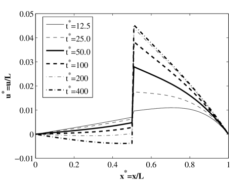
Figure 11: CZM predictions, dimensionless displacement field vs. dimensionless time.

A closer comparison with the Kapitza model can be made by comparing the CZM predictions with those predicted by the Kapitza model with the same $k_{\mathrm{int}}$. The absolute temperature gap $g_{T}$ and the normal displacement gap $g_{\mathrm{n}}$ at the interface are shown in Figs.12 and 13, respectively, as functions of time $t^{*}$.

At the very beginning of the simulation, for $g_{n}/R<l_{0}/R$, the proposed thermoelastic CZM and the Kapitza model provide the same response. Later on, the predictions of the two models diverge, due to the reduction of interface conductance related to the increased normal gap in the thermoelastic CZM.

As already observed, the thermal gap predicted by the proposed thermoelastic CZM rapidly rises. Later on, it decreases slowly until debonding takes place for $t^{*}\simeq 400$, where a small discontinuity in $g_{T}$ is observed. The Kapitza model presents a similar trend, but debonding takes place much earlier, for $t^{*}\simeq 130$.

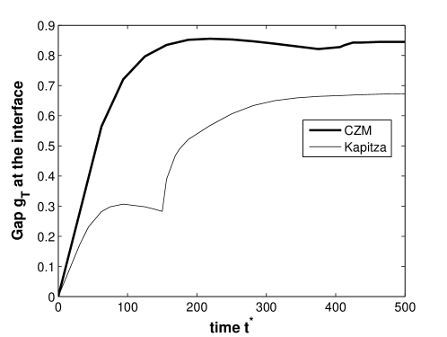
Figure 12: Temperature gap $g_{T}$ at the interface: comparison between CZM and Kapitza model.

The interface normal gap, $g_{\mathrm{n}}$ is shown in Fig. 13. After an initial matching (imputable to combined thermoelastic effects, holding also for $g_{\mathrm{n}}>l_{0}$ where the two constitutive models are different), the crack opening predicted by the proposed CZM is smaller than that by the Kapitza model, due to the reduced interface conduction. Debonding takes place at the same $g_{\mathrm{nc}}$, since the mechanical part of the CZM is the same for both simulations, but for very different times.

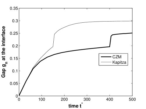
Figure 13: Normal gap $g_{\mathrm{n}}$ at the interface: comparison between CZM and Kapitza model.

Finally, the effect of the CZM parameter $\sigma_{\max}^{*}$ ($g_{\mathrm{nc}}^{*}=0.05$) is shown in Figs.14 and 15 for $t^{*}=200$. By reducing $\sigma^{*}_{\max}$, debonding takes place earlier. This is due to the competition between the strain inducted by the mechanical CZM tractions and the shrinkage due to thermal strains. For small values of $\sigma^{*}_{\max}$, the net displacement in the left part of the body is negative (thermal strain prevailing over the mechanical one) and the normal gap is amplified. For large values of $\sigma^{*}_{\max}$, the opposite situation takes place, the horizontal displacement is positive everywhere and the normal gap is reduced.

A similar trend is observed by varying $g_{\mathrm{nc}}^{*}$ keeping fixed $\sigma_{\max}^{*}=0.032$.

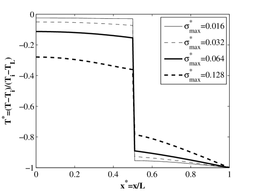
Figure 14: The effect of $\sigma_{\max}^{*}$ on the temperature field predicted by the proposed CZM.

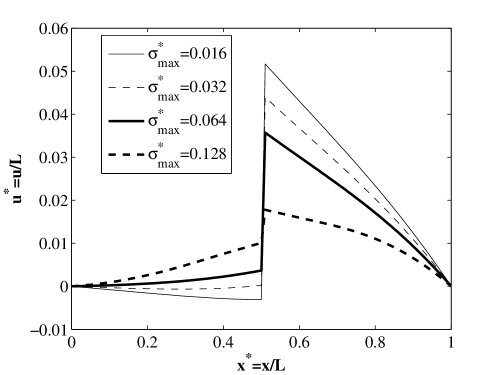
Figure 15: The effect of $\sigma_{\max}^{*}$ on the horizontal displacement field predicted by the proposed CZM.

5.3 Effect of gas conductivity

In previous studies [6, 4], the contribution of the gas to the interfacial conductivity was found to be significant. Clearly, this might depend on the problem at hand and no general rules can be put forward. To assess its effect for the present CZM formulation, the gas contribution can be included as follows:

$$q=-k_{\mathrm{int}}\Delta T+k_{\mathrm{gas}},$$ (26)

where $k_{\mathrm{gas}}$ is the gas conductivity. In the present work, we assume $k_{\mathrm{gas}}=k/1000$ as in [6, 4]. Results are shown in Fig.16. The gas contribution to the conductivity is significant only for significant crack openings and in general for $t^{*}\geq 400$. The gas conductivity has a negligible influence on the time for fracture initiation.

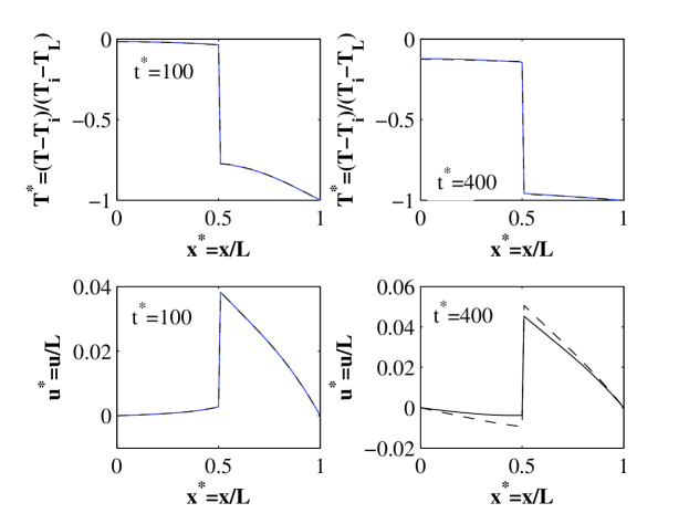
Figure 16: Effect of the gas conductivity (dashed line) on the temperature and displacement fields. Predictions without gas conductivity are shown with continuous line.

6 Application to photovoltaics

The present research on thermomechanical CZM is the continuation of the previous study in [28], where a multi-scale and multi-physics computational approach has been proposed to investigate the effect of cracking in silicon used for solar cells. Experimental results in [29] have shown that the electric conductivity of cracks is highly dependent on the temperature field. This effect is attributed both to the physics of the semiconductor whose governing equations strongly depend on the temperature, and by possible self-healing of cracks due to closing induced by thermoelastic deformation [30].

Examining the problem in more details, we know that during the production of a photovoltaic module crack-free cells made of mono- or polycrystalline silicon are laminated inside a stack composed of an encapsulating polymer and a cover glass at a temperature of about $T_{0}=150$ ^∘C. Later on, the module is brought to the environmental temperature and cracks can be inserted by handling, transport and installation operations. In proximity of a crack, the local temperature can rise significantly, leading to the so called hot spot, as evidenced in the thermal images of Fig.17.

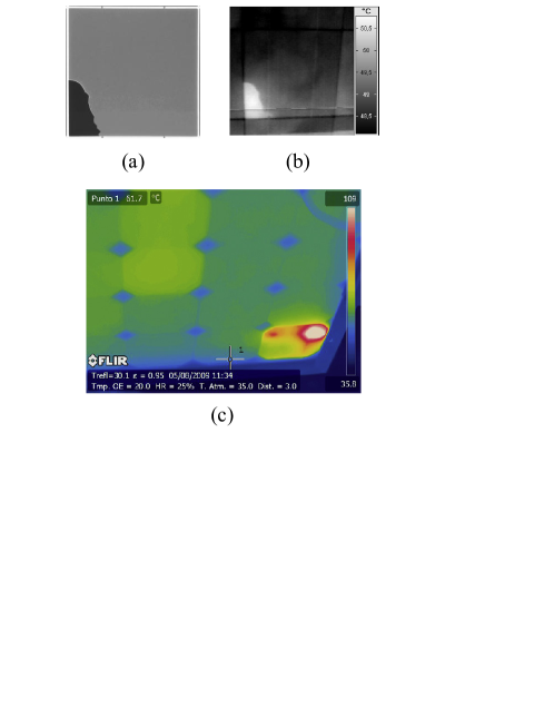
Figure 17: Thermal images obtained with a thermocamera showing local temperature rises (hot spots) in silicon cells in case of cracks ((a) and (b) adapted from [29], (c) from [31]).

As a model example, we consider a solar cell made of monocrystalline silicon with a crack on one corner, see Fig.18, similar to the real case shown in Fig.17(a). The crack is modelled by inserting interface elements along the two crack segments. The vertical sides of the cell are constrained to displacements in the horizontal direction, whereas the vertical sides are constrained in the vertical direction.

An initial temperature is applied to the cell boundaries. According to Fig.18(a), the crack separates the cell in two domains, a small one potentially insulated from the electrical point of view, $\Omega_{1}$, and the rest of the undamaged cell, $\Omega_{2}$. The whole external boundary, $\partial\Omega$, can also be partitioned into two parts: $\partial\Omega_{1}$ and $\partial\Omega_{2}$. On $\partial\Omega_{1}$, an initial temperature excursion $\Delta T_{1}=-100$ ^∘C from the stress-free state at $T=T_{0}$ is imposed, which corresponds to the jump from the lamination temperature to an operating temperature of $50$ ^∘C, to simulate the presence of a hot spot. On $\partial\Omega_{2}$, we set $\Delta T_{2}=-120$ ^∘C, i.e., a lower operating temperature of 30^∘C. Different FE meshes are considered by varying the parameter $n$, see Fig.18(b).

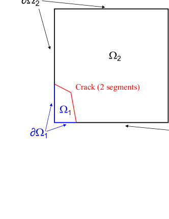
(a) Sketch of the domains separated by a crack

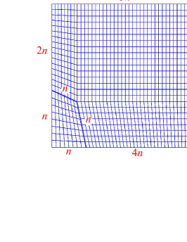
(b) FE mesh $(n=8)$

Figure 18: (a) Sketch of the geometry of a solar cell with a crack in a corner. Temperature excursions $\Delta T_{1}=-100$ ^∘C and $\Delta T_{2}=-120$ ^∘C from the reference stress-free temperature $T_{0}=150$ ^∘C are imposed along external boundaries $\partial\Omega_{1}$ and $\partial\Omega_{2}$, respectively. (b) FE mesh generated with block commands in FEAP. Different discretizations can be achieved by varying $n$.

The underlying nonlinear transient heat conduction problem is solved in order to determine the temperature distribution in the solar cell vs. time. According to the symbology introduced in Section 2, the material parameters of Silicon are $E=169$ GPa, $\nu=0.16$, $d_{m}=3100$ kg/m³, $k=114$ W/(m^∘C), $c=715$ J/(kg^∘C). The coefficient of thermal expansion is $\alpha=1.1\times 10^{-6}$ 1/C^∘. The cell thickness is $0.166$ mm. Regarding the CZM, we simulate a material with a tensile strength of about $1$ GPa, in the range of typical values reported for Silicon. The fracture energy is $G_{\mathrm{IC}}=5.92$ N/m. From this toughness and the functional form of the CZM we can deduce the values of the remaining parameters: $g_{\mathrm{nc}}=0.2\,\mu\mathrm{m}$, $R=3.135\times 10^{-2}\,\mu\mathrm{m}$, and $l_{0}=3.135\times 10^{-4}\,\mu\mathrm{m}$.

The temperature field in the solar cell is shown in Fig.19 for a sequence of times. The region of the cell in the corner, separated by the crack, tends very rapidly to a uniform temperature equal to that imposed along its boundary.

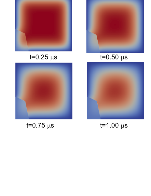
Figure 19: Time evolution of the temperature field in the solar cell with a crack in the corner. The reference stress-free temperature is $T_{0}=150$ ^∘C.

The result of a mesh convergence study by varying the parameter $n$ setting the number of interface elements per crack segment from 2 to 16 (see an example in Fig.18(b) for $n=8$) is shown in Fig.20. It depicts the temperature jump across the crack faces between region 1 (warmer) and region 2 (cooler) vs. a curvilinear coordinate moving along the two crack segments and starting from the emergent point of the crack on the vertical left side. FE solutions by varying $n$ converge very fast and the discrepancy between the solutions for $n=8$ and $n=16$ elements per crack segment is almost negligible.

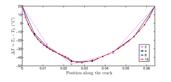
Figure 20: Mesh convergence study: temperature jump $T_{1}-T_{2}$ across the crack faces vs. position along the crack for different number of interface elements $n$ used to discretize the crack segments.

7 Conclusions

A coupled thermo-mechanical CZM derived according to an analogy with contact mechanics between rough surfaces has been proposed: the crack conductivity results to be a function of the normal cohesive tractions and the model captures the transition from the Kapitza constant resistance approach, valid for a negligible crack opening, to a crack-opening interface conductivity in case of partial debonding. Thermo-elastic effects related to the transient regime have been investigated, with particular attention to: (i) the time evolution of the temperature and displacements fields; (ii) the influence of the cohesive parameters on fracture initiation; (iii) the influence of the gas conductivity. It has also been evidenced that, neglecting thermoelastic coupling, as assumed by Kapitza’s model, very different thermal and mechanical responses are obtained. Therefore, the application of the Kapitza model to thermomechanical configurations where the phenomenon of interface debonding may occur should be checked with care.

An application to photovoltaics has been finally provided, showing the potentiality of the method to model the transient regime in the thermoelastic field in bodies containing cohesive cracks. Future perspectives of this work regard the further coupling with the electric field which, according to the physics of the solar cell, takes place in the direction orthogonal to the surface of the solar cell and is significantly influenced by cracks and defects.

Acknowledgements

The research leading to these results has received funding from the European Research Council under the European Union’s Seventh Framework Programme (FP/2007-2013)/ERC Grant Agreement No. 306622 (ERC Starting Grant Multi-field and multi-scale Computational Approach to Design and Durability of PhotoVoltaic Modules - CA2PVM). The support of the Italian Ministry of Education, University and Research to the Project FIRB 2010 Future in Research Structural mechanics models for renewable energy applications (RBFR107AKG) is gratefully acknowledged.

References

- [1] Zavarise G, Wriggers P, Stein E, Schrefler BA (1992) A numerical model for thermomechanical contact based on microscopic interface laws, International Journal for Numerical Methods in Engineering, 35, 767-785.
- [2] Song S, Yovanovich MM (1987) Explicit relative contact pressure expression: dependence upon surface roughness parameters and Vickers microhardness coefficients, AIAA Paper 87-0152.
- [3] Wriggers P, Zavarise G (1993) Thermomechanical contact–A rigorous but simple numerical approach, Computers & Structures, 46, 47-52.
- [4] Hattiangadi A, Siegmund T (2004), A thermomechanical cohesive zone model for bridged delamination cracks, Journal of the Mechanics and Physics of Solids, 52:533-566.
- [5] Hattiangadi A, Siegmund T (2005), A numerical study on interface crack growth under heat flux loading, International Journal of Solids and Structures, 42:6335-6355.
- [6] Ozdemir I, Brekelmans WAM, Geers MGD (2010), A Thermo-mechanical cohesive zone model, Computational Mechanics, 26:735-745.
- [7] Moonen P (2009) Continuous-discontinuous modelling of hygrothermal damage processes in porous media, PhD Dissertation, Catholic University of Leuven, Belgium, ISBN:978-94-6018-083-5.
- [8] Segura, JM, Carol I (2008) Coupled HM analysis using zero-thickness interface elements with double nodes. Part I: Theoretical model. International Journal for Numerical and Analytical Methods in Geomechanics, 32:2083–2101.
- [9] Secchi S, Simoni L, Schrefler BA (2007) Mesh adaptation and transfer schemes for discrete fracture propagation in porous materials. International Journal for Numerical and Analytical Methods in Geomechanics, 31:331–345.
- [10] Rethore J, de Borst R, Abellan MA (2008) A two-scale model for fluid flow in an unsaturated porous medium with cohesive cracks, Computational Mechanics, 42:227-238.
- [11] Shahil KMF, Balandin AA (2012), Graphene-multilayer graphene nanocomposites as highly efficient thermal interface materials, Nano Letters, 12:861-867.
- [12] Le-Quang H, Phan TL, Bonnet G (2011) Effective thermal conductivity of periodic composites with highly conducting imperfect interfaces, International Journal of Thermal Sciences, 50, 1428-1444.
- [13] Yvonnet J, He QC, Zhu Q-Z, Shao J-F (2011) A general and efficient computational procedure for modelling the Kapitza thermal resistance based on XFEM, Computational Materials Sciences, 50, 1220-1224.
- [14] Barber JR (2003), Bounds on the electrical resistance between contacting elastic rough bodies, Proceedings of the Royal Society of London Ser. A, 459:53-66.
- [15] Paggi M, Barber JR (2011), Contact conductance of rough surfaces composed of modified RMD patches, International Journal of Heat and Mass Transfer, 4:4664-4672.
- [16] Schellekens JCJ, de Borst R (1993) On the numerical integration of interface elements, International Journal for Numerical Methods in Engineering, 36:43–66.
- [17] Paggi M, Wriggers P (2012) A nonlocal cohesive zone model for finite thickness interfaces - Part II: FE implementation and application to polycrystalline materials, Computational Materials Science, 50:1634-1643.
- [18] Zienkiewicz OC, Taylor RL (2005) The Finite Element Method, 6th Edition, Elsevier, Oxford, UK.
- [19] Carpinteri A (1989) Cusp catastrophe interpretation of fracture instability, Journal of the Mechanics and Physics of Solids, 37:567-582.
- [20] Paggi M, Wriggers P (2011) A nonlocal cohesive zone model for finite thickness interfaces - Part I: mathematical formulation and validation with molecular dynamics, Computational Materials Science, 50:1625-1633.
- [21] Greenwood JA, Williamson JBP (1966) Contact of nominally flat surfaces, Proceedings of the Royal Society of London Ser. A, 295:300-319.
- [22] Lorenz B, Persson BNJ (2008) Interfacial separation between elastic solids with randomly rough surfaces: comparison of experiment with theory, Journal of Physics of Condensed Matter 21:015003.
- [23] Kubair DV, Geubelle PH (2003) Comparative analysis of extrinsic and intrinsic cohesive models of dynamic fracture, International Journal of Solids and Structures, 40:3853-3868.
- [24] Allix O, Corigliano A (1996) Modeling and simulation of crack propagation in mixed-modes interlaminar fracture specimens, International Journal of Fracture, 77:111-140.
- [25] Xu X, Needleman A (1994) Numerical simulations of fast crack growth in brittle solids, Journal of the Mechanics and Physics of Solids, 42:1397-1434.
- [26] van den Bosch MJ, Schreurs PJG, Geers MGD (2006) An improved definition of the exponential Xu and Needlman cohesive zone law for mixed-mode decohesion, Engineering Fracture Mechanics, 73:1220-1234.
- [27] Paggi M, Wriggers P (2012) Stiffness and strength of hierarchical polycrystalline materials with imperfect interfaces, Journal of the Mechanics and Physics of Solids, 60:557–571.
- [28] Paggi M, Corrado M, Rodriguez MA (2013) A multi-physics and multi-scale numerical approach to microcracking and power-loss in photovoltaic modules, Composite Structures, 95:630-638.
- [29] Weinreich B, Schauer B, Zehner M, Becker G (2012) Validierung der Vermessung gebrochener Zellen im Feld mittels Leistungs PV-Thermographie. In: Tagungsband 27. Symposium Photovoltaische Solarenergie, Bad Staffelstein, Germany, 190–196.
- [30] Paggi M, Sapora A (2013) Numerical modelling of microcracking in PV modules induced by thermo-mechanical loads, Energy Procedia, 38:506-515.
- [31] Munoz MA, Alonso-Garcia MC, Vela N, Chenlo F (2011) Early degradation of silicon PV modules and guaranty conditions. Solar Energy, 85:2264–2274.