Multiscale Temporal Integrators for Fluctuating Hydrodynamics

Abstract

Following on our previous work [S. Delong and B. E. Griffith and E. Vanden-Eijnden and A. Donev, Phys. Rev. E, 87(3):033302, 2013], we develop temporal integrators for solving Langevin stochastic differential equations that arise in fluctuating hydrodynamics. Our simple predictor-corrector schemes add fluctuations to standard second-order deterministic solvers in a way that maintains second-order weak accuracy for linearized fluctuating hydrodynamics. We construct a general class of schemes and recommend two specific schemes: an explicit midpoint method, and an implicit trapezoidal method. We also construct predictor-corrector methods for integrating the overdamped limit of systems of equations with a fast and slow variable in the limit of infinite separation of the fast and slow timescales. We propose using random finite differences to approximate some of the stochastic drift terms that arise because of the kinetic multiplicative noise in the limiting dynamics. We illustrate our integrators on two applications involving the development of giant nonequilibrium concentration fluctuations in diffusively-mixing fluids. We first study the development of giant fluctuations in recent experiments performed in microgravity using an overdamped integrator. We then include the effects of gravity, and find that we also need to include the effects of fluid inertia, which affects the dynamics of the concentration fluctuations greatly at small wavenumbers.

I Introduction and Background

Fluctuating Hydrodynamics (FHD) accounts for stochastic effects arising at mesoscopic and macroscopic scales because of the discrete nature of fluids at microscopic scales Landau:Fluid ; LLNS_FD_Fox ; FluctHydroNonEq_Book . In FHD, spatially-extended Langevin equations are constructed by including stochastic flux terms in the classical Navier-Stokes-Fourier equations of fluid dynamics and related conservation laws. It is widely appreciated that thermal fluctuations are important in flows at micro and nano scales; even more importantly, hydrodynamic fluctuations span the whole range of scales from the microscopic to the macroscopic and need to be consistently included in all levels of description GiantFluctuations_Nature ; DropletSpreading ; FractalDiffusion_Microgravity ; DiffusionJSTAT . While the original formulation of fluctuating hydrodynamics was for compressible single-component fluids Landau:Fluid , the methodology can be extended to other systems such as fluid mixtures FluctHydroNonEq_Book , chemically reactive systems FluctuatingReactionDiffusion , magnetic materials FluctHydro_Magnetic , and others LebowitzHydroReview . The structure of the equations of fluctuating hydrodynamics can be, to some extent, justified on the basis of the Mori-Zwanzig formalism LLNS_Espanol ; DiscreteLLNS_Espanol . The basic idea is to add a stochastic flux corresponding to each dissipative (irreversible, diffusive) flux, leading to a continuum Langevin model that ensures detailed balance with respect to a suitable Einstein or Gibbs-Boltzmann equilibrium distribution OttingerBook .

After spatial discretization (truncation) of the stochastic partial differential equations (SPDEs) of FHD, one obtains a large-scale system of stochastic ordinary differential equations (SODEs) that has the familiar structure of Langevin equations common in statistical mechanics. The spatial discretization must be performed with specific attention to preserving fluctuation-dissipation balance DFDB ; alternatively, one can directly construct discrete Langevin equations with the proper structure from the underlying microscopic dynamics by using the theory of coarse-graining DiscreteDiffusion_Espanol ; DiscreteLLNS_Espanol . In this paper, continuing on our previous work DFDB , we are concerned with temporal integration of the Langevin systems that arise in fluctuating hydrodynamics and other mesoscopic models. In DFDB , we constructed several simple predictor-corrector (two-step) schemes for Langevin equations and applied them to the incompressible fluctuating hydrodynamics equations coupled with an advection-diffusion equation for a scalar concentration field. The main feature of these schemes is that they allow one to treat some terms implicitly (e.g., mass or momentum diffusion), and treat others explicitly (e.g, advection). Furthermore, the schemes presented in DFDB are second-order weakly accurate for nonlinear SODEs with constant additive noise, while also achieving, in certain cases, third-order accuracy for the static correlation functions (static structure factors in fluctuating hydrodynamics).

In practical applications, however, several difficulties arise that require the development of novel temporal integration schemes. The first complication in FHD is the appearance of multiplicative noise. In the context of SPDEs, such multiplicative noise is often purely formal and cannot be interpreted mathematically in continuum formulations unless the nonlinear terms are regularized DiffusionJSTAT ; DDFT_Hydro , or suitable renormalization terms are added RegularityStructures . In most cases, a precise formulation of the multiplicative noise terms is not known and the importance of various stochastic drift terms arising due to the multiplicative nature of the noise have not been explored. A precise mathematical interpretation can, however, be given to the equations of linearized FHD (LFHD), which are in fact the most common model used in the literature FluctHydroNonEq_Book . The LFHD equations can in some cases be derived rigorously from the microscopic dynamics as a form of central limit theorem for the Gaussian fluctuations around the deterministic hydrodynamic equations, which are themselves a form of law of large numbers for the macroscopic observables LebowitzHydroReview ; MicroToSPDE_Review ; AERW_Varadhan ; LDT_Excluded ; LLN_InteractingBrownian . One can, at least formally, obtain the LFHD equations from the nonlinear FHD equations by expanding to leading order in the magnitude of the stochastic forcing terms (more precisely, the inverse of the coarse-graining length scale).

Such linearization of nonlinear FHD equations leads to a system of two equations, the usual nonlinear deterministic equation, and a linear (additive-noise) stochastic differential equation (SDE) for the Gaussian fluctuations around the mean. A naive application of the temporal integrators in DFDB would require first solving the deterministic equation, itself a nontrivial problem except in the simplest of cases, and then solving a linear SDE with a time-dependent but additive noise of magnitude determined by the deterministic solution. Here we demonstrate that with some simple modifications the predictor-corrector integrators from DFDB can accomplish these two steps together without ever explicitly writing the LFHD equations. Specifically, here we construct schemes that numerically linearize the equations around a numerically-determined deterministic solution. Our analysis shows how to achieve second-order weak accuracy for the LFHD equations by choosing where to evaluate the amplitude of the stochastic forcing terms. In certain cases, the resulting integrators will also be first-order weakly accurate for the (discrete or regularized) nonlinear FHD equations. For nonlinear Langevin equations with multiplicative noise, in general, it is difficult to construct integrators of weak order higher than one. Second-order weak Runge-Kutta (derivative-free) schemes have been constructed WeakSecondOrder_RK for systems of SODEs, however, using these types of methods in the contexts of SPDEs is non trivial.

A second difficulty that often arises in FHD is the appearance of large separation of time scales between the different hydrodynamic variables. In incompressible FHD, velocity fluctuations are the most rapid, since flows at small scales are typically viscous-dominated and momentum diffuses much faster than does mass. As the dynamics of interest is usually the slow dynamics of the concentration field or discrete particles advected by the velocity fluctuations, specialized multiscale temporal integrators are required to avoid the need to use small time step sizes that resolve the fast dynamics. This can be accomplished by analytically performing adiabatic mode elimination and eliminating the fast variable from the description to obtain a limiting or overdamped equation for the slow variables, and then numerically integrating the limiting dynamics. In this work we develop predictor-corrector schemes that in essence numerically take the overdamped limit of a two-scale (fast-slow) system of SODEs in which the fast variable enters linearly. Our predictor-corrector schemes are applicable to a broad range of two-scale Langevin equations that frequently arise in practice in a variety of contexts. Their key feature is that they obtain all of the stochastic drift terms numerically without requiring derivatives. This makes it relatively easy to take a code that integrates the original fast-slow inertial dynamics using a (semi-)implicit method, and to convert it into a code that integrates the overdamped dynamics. Furthermore, the schemes we construct here are second-order weakly accurate for the linearized overdamped equations. In order to facilitate the integration of our methods in existing codes our algorithms make use of the components already required to integrate the original fast-slow equations without making use of the large-separation of scales. The result is a new algorithm that reuses the base code but can take a time step several orders of magnitude larger.

In this work we demonstrate that simple predictor-corrector methods can address the difficulties discussed above with a minimal amount of effort on the part of the user. Specifically, we develop simple predictor-corrector schemes for temporal integration of Langevin SDEs that arise in fluctuating hydrodynamics and accomplish the following design goals:

1. They reuse the same computational components already available in standard computational fluid dynamics (CFD) solvers, such as linear solvers for viscosity or diffusion, advection schemes, etc.

2. In the deterministic context they are second-order accurate and relatively standard.

3. For nonlinear but additive noise SDEs they are second-order weakly accurate DFDB .

4. They numerically linearize the FHD equations and solve the LFHD equations weakly to second-order.

5. For LFHD, they give higher-order accurate static correlations (static structure factors) at steady state DFDB .

6. They can be used to integrate two-scale fast-slow systems in the overdamped limit, preserving all of the above properties but now referring to the limiting dynamics.

7. In the general nonlinear multiplicative-noise case, they are weakly first-order accurate and do not require any derivative information.

Some of us have previously made use of some of the temporal integrators described here in more specialized works. In BrownianBlobs we constructed temporal integrators for the equations of Brownian Dynamics, which is a multiplicative-noise overdamped SDE. These overdamped Langevin equations result when one eliminates the fast velocity degrees of freedom from a system of equations for the motion of particles immersed in a fluctuating Stokes fluid. In DiffusionJSTAT we solved a related overdamped SPDE for the concentration of the immersed particles DDFT_Hydro using the techniques detailed here. In LowMachImplicit we apply our methods to the low Mach number equations of FHD. In this work we present the temporal integrators used in this prior work in greater generality, with the hope that they will be useful for other Langevin equations. We also explain the analysis required to study the order of weak accuracy of the schemes, making it easier for other researchers to further generalize our methods or to apply them in specific contexts.

The remainder of this section discusses Langevin equations and a specific example thereof: the equations of fluctuating hydrodynamics. In section II we introduce schemes that are second order weakly accurate for the linearized (weak noise limit) Langevin equations. Section III studies systems of equations with a fast and slow variable and proposes schemes which perform adiabatic elimination of the fast variable numerically. Section IV outlines specific versions of our schemes applied to a system of passive tracers advected by a fluctuating fluid, and in section V, we use our temporal integration methods to simulate diffusive mixing in binary liquid mixtures. Finally, section VI gives our concluding thoughts and remarks.

I.1 Generic Langevin equations

As discussed in more detail in our previous work DFDB , we consider temporal integrators for a class of generic Langevin equations for the coarse-grained variables $\boldsymbol{x}\left(t\right)$ GrabertBook ,

$$\partial_{t}\boldsymbol{x}=-\boldsymbol{N}\left(\boldsymbol{x}\right)\frac{\partial U}{\partial\boldsymbol{x}}+\left(2k_{B}T\right)^{1/2}\boldsymbol{M}_{\frac{1}{2}}\left(\boldsymbol{x}\right)\,\boldsymbol{\mathcal{W}}(t)+\left(k_{B}T\right)\frac{\partial}{\partial\boldsymbol{x}}\cdot\boldsymbol{N}\left(\boldsymbol{x}\right),$$ (1)

where $\boldsymbol{\mathcal{W}}(t)$ denotes white noise, the formal time derivative of a collection of independent Brownian motions, and an Ito interpretation is assumed. Here $U\left(\boldsymbol{x}\right)$ is the thermodynamic driving potential, such as an externally-applied conservative potential or a coarse-grained free energy. We will typically suppress the explicit dependence on $\boldsymbol{x}$ and write the mobility operator as $\boldsymbol{N}\equiv\boldsymbol{N}\left(\boldsymbol{x}\right)$, and assume that the noise operator $\boldsymbol{M}_{\frac{1}{2}}\left(\boldsymbol{x}\right)$ obeys the fluctuation-dissipation balance condition

$$\boldsymbol{M}_{\frac{1}{2}}\boldsymbol{M}_{\frac{1}{2}}^{\star}=\boldsymbol{M}=\frac{1}{2}\left(\boldsymbol{N}+\boldsymbol{N}^{\star}\right),$$ (2)

where star denotes an adjoint. This ensures that the dynamics (1) is (under suitable assumptions) ergodic with respect to the Gibbs-Boltzmann distribution

$$P_{\text{eq}}\left(\boldsymbol{x}\right)=Z^{-1}\,\exp\left[-\frac{U\left(\boldsymbol{x}\right)}{k_{B}T}\right],$$ (3)

where $Z$ is a normalization constant. In the notation we have chosen, in component form $\left(\partial_{\boldsymbol{x}}\cdot\boldsymbol{N}\right)_{i}=\partial_{j}N_{ij}$, where repeated indices are implicitly summed throughout this paper. Please note that this is different from the less-standard notation we used in our previous paper DFDB , where the drift term is written as $\left(k_{B}T\right)\,\partial_{\boldsymbol{x}}\cdot\boldsymbol{N}^{\star}$.

The last term in (1) is an additional “stochastic” or “thermal” drift term, as can be seen from the fact that it is proportional to $k_{B}T$. This term contains information about the noise and therefore depends on the particular interpretation of the stochastic integral. The thermal drift term, however, also contains information about the anti-symmetric part of the generator $\boldsymbol{N}$ that is unrelated to the stochastic noise term. If the skew-adjoint component $\boldsymbol{L}=\frac{1}{2}\left(\boldsymbol{N}^{\star}-\boldsymbol{N}\right)$ is divergence-free, $\partial_{\boldsymbol{x}}\cdot\boldsymbol{L}=0$, the associated dynamics is incompressible in phase space AugmentedLangevin and the stochastic drift term disappears if one uses the kinetic interpretation KineticStochasticIntegral_Ottinger of the stochastic integral, denoted with the stochastic product $\diamond$,

$$\partial_{t}\boldsymbol{x}=-\boldsymbol{N}\left(\boldsymbol{x}\right)\frac{\partial U}{\partial\boldsymbol{x}}+\left(2k_{B}T\right)^{1/2}\boldsymbol{M}_{\frac{1}{2}}\left(\boldsymbol{x}\right)\diamond\boldsymbol{\mathcal{W}}(t).$$ (4)

In the case when $\boldsymbol{N}=\boldsymbol{M}$ is self-adjoint, $\boldsymbol{L}=0$, the kinetic SDE (4) corresponds to a Fokker-Planck equation for the evolution of the probability distribution $P\left(\boldsymbol{x},t\right)$ for observing the state $\boldsymbol{x}$ at time $t$,

$$\frac{\partial P}{\partial t}=\frac{\partial}{\partial\boldsymbol{x}}\cdot\left\{\boldsymbol{M}\left[\frac{\partial U}{\partial\boldsymbol{x}}P+\left(k_{B}T\right)\frac{\partial P}{\partial\boldsymbol{x}}\right]\right\},$$ (5)

where we note that the term in square brackets vanishes when $P=P_{eq}$.

I.2 Overdamped Langevin equation

As a simple but illustrative example of a Langevin equation that our methods can be applied to we consider the Langevin equation with position-dependent friction tensor $\boldsymbol{\gamma}\left(\boldsymbol{x}\right)$,

$$m\partial_{t}\boldsymbol{v} =\boldsymbol{F}\left(\boldsymbol{x}\right)-\boldsymbol{\gamma}\left(\boldsymbol{x}\right)\boldsymbol{v}+\sqrt{2k_{B}T\boldsymbol{\gamma}\left(\boldsymbol{x}\right)}\,\boldsymbol{\mathcal{W}}\left(t\right)$$

$$\partial_{t}\boldsymbol{x} =\boldsymbol{v},$$ (6)

where $\boldsymbol{x}(t)$ is the position of a particle diffusing under the influence of an external force $\boldsymbol{F}(\boldsymbol{x})=-\partial_{\boldsymbol{x}}U(\boldsymbol{x})$, $\boldsymbol{v}(t)$ is the particle velocity, and $m$ is its mass. It is well-known that in the low-inertia limit $m\rightarrow 0$, the velocity can be eliminated as a fast degree of freedom to obtain the overdamped Langevin equation ModeElimination_Papanicolaou ; AveragingHomogenization

$$\partial_{t}\boldsymbol{x}=\boldsymbol{\gamma}^{-1}\left(\boldsymbol{x}\right)\boldsymbol{F}\left(\boldsymbol{x}\right)+\sqrt{2k_{B}T}\,\boldsymbol{\gamma}^{-\frac{1}{2}}\left(\boldsymbol{x}\right)\boldsymbol{\mathcal{W}}\left(t\right)+\left(k_{B}T\right)\partial_{\boldsymbol{x}}\cdot\boldsymbol{\gamma}^{-1}\left(\boldsymbol{x}\right),$$ (7)

which is of the form (1) with a self-adjoint mobility $\boldsymbol{N}=\boldsymbol{M}\equiv\boldsymbol{\gamma}^{-1}$ and with $\boldsymbol{M}^{\frac{1}{2}}\equiv\boldsymbol{\gamma}^{-\frac{1}{2}}$ being a matrix square root or a Cholesky factor of $\boldsymbol{\gamma}^{-1}$. Even though the overdamped equation strictly only applies in the limit of infinite separation of time scales, it will be a very good approximation so long as there still remains a large separation of time scales between the fast velocity and the slow position.

I.2.1 Fixman Scheme

In this paper we construct predictor-corrector algorithms that integrate the overdamped equation (7) by instead directly discretizing the inertial equation (6) without the inertial term $\partial_{t}\boldsymbol{v}$. By carefully constructing the corrector stage we will obtain the correct stochastic or thermal drift term in (7). For the simple Langevin equation (6) a trapezoidal integrator goes from time step $n$ to time step $n+1$ via the two stages,

$$\boldsymbol{\gamma}^{n}\boldsymbol{v}^{n}= \boldsymbol{F}^{n}+\sqrt{\frac{2k_{B}T}{\Delta t}}\ \left(\boldsymbol{\gamma}^{n}\right)^{\frac{1}{2}}\boldsymbol{W}^{n}$$

$$\boldsymbol{x}^{p,n+1}= \boldsymbol{x}^{n}+\boldsymbol{v}^{n}\Delta t\quad\mbox{(predictor)}$$ (8)

$$\boldsymbol{\gamma}^{p,n+1}\boldsymbol{v}^{p,n+1}= \boldsymbol{F}^{p,n+1}+\sqrt{\frac{2k_{B}T}{\Delta t}}\ \left(\boldsymbol{\gamma}^{n}\right)^{\frac{1}{2}}\boldsymbol{W}^{n}$$

$$\boldsymbol{x}^{n+1}= \boldsymbol{x}^{n}+\left(\frac{\boldsymbol{v}^{n}+\boldsymbol{v}^{p,n+1}}{2}\right)\Delta t\quad\mbox{(corrector)},$$ (9)

where superscripts denote the point at which a given quantity is evaluated, for example, $\boldsymbol{\gamma}^{p,n+1}=\boldsymbol{\gamma}\left(\boldsymbol{x}^{p,n+1}\right)$, and $\boldsymbol{W}^{n}$ is a collection of independent and identically distributed (i.i.d.) standard normal random variables sampled independently at each time step. This predictor-corrector method is only first-order accurate for the multiplicative-noise case. When one is interested in linearized equations (e.g., a particle trapped by a harmonic potential to remain close to a stable minimum of the potential) the predictor-corrector schemes we construct in section III are second-order weakly accurate. It is not hard to show that the scheme (9) is equivalent to the well-known Fixman integrator for (7) BD_Fixman .

Note that the final Fixman update can be written in the form

$$\boldsymbol{x}^{n+1} = \boldsymbol{x}^{n}+\left(\frac{\boldsymbol{M}^{n}\boldsymbol{F}^{n}+\boldsymbol{M}^{p,n+1}\boldsymbol{F}^{p,n+1}}{2}\right)\Delta t+\sqrt{2k_{B}T\Delta t}\,\left(\boldsymbol{M}^{n}\right)^{\frac{1}{2}}\boldsymbol{W}^{n},$$ (10)

$$+ \Delta t\left(k_{B}T\right)\left(\boldsymbol{M}^{p,n+1}-\boldsymbol{M}^{n}\right)\left(2k_{B}T\Delta t\,\boldsymbol{M}^{n}\right)^{-\frac{1}{2}}\boldsymbol{W}^{n},$$

where the mobility $\boldsymbol{M}=\boldsymbol{\gamma}^{-1}$. The first line is seen as an application of the (second-order) explicit trapezoidal rule for the deterministic drift terms and the Euler-Maryama method for the stochastic terms, while the second line gives the thermal drift term $\Delta t\left(k_{B}T\right)\partial_{\boldsymbol{x}}\cdot\boldsymbol{M}(\boldsymbol{x})$ in expectation, as we explain next.

I.2.2 Random Finite Difference

A key feature of the Fixman method is that it requires access to the action of both $\boldsymbol{\gamma}^{-1}$ and $\boldsymbol{\gamma}^{\frac{1}{2}}$, or equivalently, $\boldsymbol{\gamma}$ and $\boldsymbol{\gamma}^{-\frac{1}{2}}$. This is a great disadvantage in cases when only the action of the mobility $\boldsymbol{M}=\boldsymbol{\gamma}^{-1}$ and its factor $\boldsymbol{M}^{\frac{1}{2}}$ are easily computable BrownianBlobs . An alternative method to obtain the drift term $\left(k_{B}T\right)\partial_{\boldsymbol{x}}\cdot\boldsymbol{M}\left(\boldsymbol{x}\right)$ in expectation is to use the general relation,

$$\lim_{\delta\rightarrow 0}\frac{1}{\delta}\left\langle\left(\boldsymbol{M}\left(\boldsymbol{x}+\delta\Delta\boldsymbol{x}\right)-\boldsymbol{M}\left(\boldsymbol{x}\right)\right)\Delta\boldsymbol{p}\right\rangle=\partial_{\boldsymbol{x}}\cdot\boldsymbol{M}(\boldsymbol{x}),$$ (11)

where $\Delta\boldsymbol{x}$ and $\Delta\boldsymbol{p}$ are Gaussian variates with mean zero and covariance $\left\langle\Delta\boldsymbol{x}_{i}\Delta\boldsymbol{p}_{j}\right\rangle=\delta_{ij}$. The second line in the Fixman method (10) can be seen as an application of (11) with $\delta=\sqrt{\Delta t}$ and $\Delta\boldsymbol{x}=\left(2k_{B}T\,\boldsymbol{M}^{n}\right)^{\frac{1}{2}}\boldsymbol{W}^{n}$ and $\Delta\boldsymbol{p}=\left(2k_{B}T\,\boldsymbol{M}^{n}\right)^{-\frac{1}{2}}\boldsymbol{W}^{n}$. The choice $\Delta\boldsymbol{x}=\Delta\boldsymbol{p}$ is, however, much simpler to use than the Fixman choice because it does not require the application of either $\left(\boldsymbol{M}^{n}\right)^{\frac{1}{2}}$ or $\left(\boldsymbol{M}^{n}\right)^{-\frac{1}{2}}$. Here $\delta$ is a small discretization parameter that can be taken to be related to $\Delta t$ as in the Fixman method, but this is not necessary. One can more appropriately think of (11) as a “random finite difference” (RFD) with $\delta$ representing the small spacing for the finite difference, to be taken as small as possible while avoiding numerical roundoff problems. The advantage of the “random” over a traditional finite difference is that only a small number of evaluations of the mobility per time step is required. Note that the subtraction of $\boldsymbol{M}\left(\boldsymbol{x}\right)\Delta\boldsymbol{p}$ in (11) is necessary in order to control the variance of the RFD estimate.

For the simple Langevin equation (6) an RFD approach uses the same predictor (8) as in the Fixman algorithm, but now with corrector,

$$\boldsymbol{v}^{p,n+1}= \left(\boldsymbol{\gamma}^{p,n+1}\right)^{-1}\boldsymbol{F}^{p,n+1}+\sqrt{\frac{2k_{B}T}{\Delta t}}\ \left(\boldsymbol{\gamma}^{n}\right)^{-\frac{1}{2}}\boldsymbol{W}^{n}$$

$$\boldsymbol{x}^{n+1}= \boldsymbol{x}^{n}+\left(\frac{\boldsymbol{v}^{n}+\boldsymbol{v}^{p,n+1}}{2}\right)\Delta t$$

$$+ \left(k_{B}T\right)\frac{\Delta t}{\delta}\left[\boldsymbol{\gamma}^{-1}\left(\boldsymbol{x}^{n}+\delta\,\widetilde{\boldsymbol{W}}^{n}\right)-\boldsymbol{\gamma}^{-1}\left(\boldsymbol{x}^{n}\right)\right]\widetilde{\boldsymbol{W}}^{n},$$ (12)

where $\widetilde{\boldsymbol{W}}^{n}$ is a collection of independent standard normal variates that are uncorrelated with $\boldsymbol{W}^{n}$. Because the corrector stage for the velocity evaluates the noise amplitude at the beginning of the time step there are no stochastic drift terms generated from the term $\left(\boldsymbol{v}^{n}+\boldsymbol{v}^{p,n+1}\right)\Delta t/2$, and the RFD in the last line of (12) is necessary to generate the missing drift in expectation.

It is not hard to see that (12) is a Markov chain that is consistent with the Ito overdamped equation (7). To demonstrate consistency we only need to show that to leading order, the first moment of the increment is equal to the deterministic drift in expectation,

$$\lim_{\Delta t\rightarrow 0}\frac{1}{\Delta t}\,E\left(\boldsymbol{x}^{n+1}-\boldsymbol{x}^{n}\right)=\boldsymbol{M}^{n}\boldsymbol{F}^{n}+\left(k_{B}T\right)\partial_{\boldsymbol{x}}\cdot\boldsymbol{M}(\boldsymbol{x}^{n}),$$

which follows directly from (11), and that in expectation the second moment of the increment matches the covariance of the noise,

$$\lim_{\Delta t\rightarrow 0}\frac{1}{\Delta t}\,E\left(\left(\boldsymbol{x}^{n+1}-\boldsymbol{x}^{n}\right)\left(\boldsymbol{x}^{n+1}-\boldsymbol{x}^{n}\right)^{T}\right)=2k_{B}T\,\boldsymbol{M}^{n},$$

which is trivially true because the random increment in both the predictor and corrector stages is $\sqrt{2k_{B}T\Delta t}\,\left(\boldsymbol{M}^{n}\right)^{\frac{1}{2}}\boldsymbol{W}^{n}$.

The two schemes (8,9) and (8,12) do not, of course, exhaust all possibilities. For example, in the corrector stage for velocity we could evaluate the noise amplitude at the predicted value,

$$\boldsymbol{v}^{p,n+1}=\left(\boldsymbol{\gamma}^{p,n+1}\right)^{-1}\boldsymbol{F}^{p,n+1}+\sqrt{\frac{2k_{B}T}{\Delta t}}\ \left(\boldsymbol{\gamma}^{p,n+1}\right)^{-\frac{1}{2}}\boldsymbol{W}^{n}.$$

It is not difficult to show, however, that with this choice the term $\left(\boldsymbol{v}^{n}+\boldsymbol{v}^{p,n+1}\right)\Delta t/2$ in the corrector stage for the position would generate an incorrect stochastic drift term for non-scalar problems. Therefore, additional RFD terms would be required to remove any spurious drift terms and add the correct ones. In this work we construct several schemes for integrating two-scale systems such as (7) that generate the correct drift terms using random finite differences, and, furthermore, also obtain second-order weak accuracy for the overdamped equations linearized around a stable deterministic trajectory. With additional effort, it is also possible to obtain second-order weak accuracy for the nonlinear overdamped equation by using weak Runge-Kutta schemes of the kind developed in WeakSecondOrder_RK , which also rely on an RFD-like approach to avoid explicit evaluation of derivatives.

I.3 Fluctuating Hydrodynamics

As a motivating example of a fluctuating hydrodynamic system of equations to which our methods will be applied, we study a model of diffusion of tagged (labeled) molecules in a liquid or of colloidal particles suspended in a fluid. A detailed mesoscopic model for diffusion in liquids has been described by some of us in previous work DiffusionJSTAT ; DDFT_Hydro ; here we only summarize some key points to give a specific setting for the discussion to follow. The hydrodynamic fluctuations of the fluid velocity $\boldsymbol{v}\left(\boldsymbol{r},t\right)$ will be modeled via the incompressible fluctuating Navier-Stokes equation, $\boldsymbol{\nabla}\cdot\boldsymbol{v}=0$, and

$$\rho\left(\partial_{t}\boldsymbol{v}+\boldsymbol{v}\cdot\boldsymbol{\nabla}\boldsymbol{v}\right)+\boldsymbol{\nabla}\pi=\eta\boldsymbol{\nabla}^{2}\boldsymbol{v}+\boldsymbol{\nabla}\cdot\left(\sqrt{2\eta k_{B}T}\,\boldsymbol{\mathcal{W}}\right)-\beta\rho c\,\boldsymbol{g},$$ (13)

and appropriate boundary conditions. Here $\rho$ is the fluid density, $\eta=\rho\nu$ the shear viscosity, and $T$ the temperature, all assumed to be constant throughout the domain, and $\pi\left(\boldsymbol{r},t\right)$ is the mechanical pressure. The last term in this equation models the effects of gravity using a Boussinesq constant density approximation, with $\boldsymbol{g}$ being the gravitational acceleration, and $\beta$ the solutal expansion coefficient. The concentration of diffusing particles is given by the mass fraction $c\left(\boldsymbol{r},t\right)=\left(m/\rho\right)n\left(\boldsymbol{r},t\right)$, where $n$ is the number density and $m$ is the mass of the tracer particles. The stochastic momentum flux is modeled via a white-noise symmetric tensor field $\boldsymbol{\mathcal{W}}\left(\boldsymbol{r},t\right)$ with covariance chosen to obey a fluctuation-dissipation principle FluctHydroNonEq_Book ; OttingerBook ,

$$\left\langle\mathcal{W}_{ij}(\boldsymbol{r},t)\mathcal{W}_{kl}(\boldsymbol{r}^{\prime},t^{\prime})\right\rangle=\left(\delta_{ik}\delta_{jl}+\delta_{il}\delta_{jk}\right)\delta(t-t^{\prime})\delta(\boldsymbol{r}-\boldsymbol{r}^{\prime}).$$

Note that because the noise is additive in (13) there is no difference between an Ito and a Stratonovich interpretation of the stochastic term. For technical reasons, in this work we will drop the nonlinear advective term $\boldsymbol{v}\cdot\boldsymbol{\nabla}\boldsymbol{v}$ and consider the time-dependent fluctuating Stokes equation; this is a good approximation since this term only plays an important role at very large scales.

For our purposes, we will model the evolution of the concentration $c\left(\boldsymbol{r},t\right)$ via a fluctuating advection-diffusion Ito equation SPDE_Diffusion_Dean ; DDFT_Hydro ,

$$\partial_{t}c+\boldsymbol{u}\cdot\boldsymbol{\nabla}c=\chi_{0}\boldsymbol{\nabla}^{2}c+\boldsymbol{\nabla}\cdot\left(\sqrt{2\chi_{0}\rho^{-1}mc}\,\boldsymbol{\mathcal{W}}_{c}\right),$$ (14)

where $\boldsymbol{\mathcal{W}}_{c}\left(\boldsymbol{r},t\right)$ denotes a white-noise vector field. Here $\chi_{0}$ is a bare or molecular diffusion coefficient, and the concentration is advected by the random field

$$\boldsymbol{u}\left(\boldsymbol{r},t\right)=\int\boldsymbol{\sigma}\left(\boldsymbol{r},\boldsymbol{r}^{\prime}\right)\boldsymbol{v}\left(\boldsymbol{r}^{\prime},t\right)d\boldsymbol{r}^{\prime}\equiv\boldsymbol{\sigma}\star\boldsymbol{v},$$ (15)

where $\boldsymbol{\sigma}$ is a smoothing kernel that filters out features at scales below a microscopic (molecular) scale $\sigma$, and $\star$ denotes convolution. It is important here that $\boldsymbol{u}$ is also divergence-free, $\boldsymbol{\nabla}\cdot\boldsymbol{u}=0$. Formally, one often writes the advective term in (14) as $\boldsymbol{v}\cdot\boldsymbol{\nabla}c$ (this corresponds to $\boldsymbol{\sigma}\left(\boldsymbol{r},\boldsymbol{r}^{\prime}\right)=\delta\left(\boldsymbol{r}-\boldsymbol{r}^{\prime}\right)$) but this only makes sense if one truncates the velocity equation (13) at some ultraviolet cutoff wave number $k_{\text{max}}\sim\sigma^{-1}$; this kind of implicit smoothing kernel is applied by the finite-volume spatial discretization we employ DFDB , with the grid spacing playing the role of $\sigma$. Additional filtering may also be implemented in the finite-volume schemes, as described in Appendix B in LowMachExplicit . The system of equations (13,14) is a useful model, for example, for the study of giant concentration fluctuations in low-density polymer FractalDiffusion_Microgravity or nanocolloidal suspensions GiantFluct_NanoColloids , or in binary fluid mixtures in the presence of a modest temperature gradient SoretDiffusion_Croccolo .

It can be shown that the coupled velocity-concentration system (13,14) can formally be written as an infinite-dimensional system of the form (1) with a physically-sensible coarse-grained energy functional

$$U\left[\boldsymbol{v}\left(\cdot\right),\,c\left(\cdot\right)\right]=\frac{\rho}{2}\int v^{2}\left(\boldsymbol{r}\right)\,d\boldsymbol{r}+\beta\rho\int c\left(\boldsymbol{r}\right)\left(\boldsymbol{r}\cdot\boldsymbol{g}\right)\,d\boldsymbol{r}+\left(k_{B}T\right)\int n\left(\boldsymbol{r}\right)\left(\ln\left(\Lambda^{3}n\left(\boldsymbol{r}\right)\right)-1\right)\,d\boldsymbol{r},$$ (16)

where $n=\rho c/m$ is the number density of the diffusing particles, and $\Lambda$ is a fixed length-scale (e.g., the thermal de Broglie wavelength). A specific form of the mobilty operator can also be written, see for example Refs. DFDB for the advective terms and Ref. DDFT_Hydro for the diffusive and stochastic terms. Numerical methods for integrating systems such (13,14) as have been discussed in Refs. LLNS_Staggered ; LowMachExplicit ; DFDB . In particular, after spatial discretization of the system of SPDEs (13,14) one obtains a system of SODEs of the generic Langevin form (1). We note that the last term in (16), which contains the free energy density of an ideal gas with number density $c\left(\boldsymbol{r}\right)$, is quite formal and poses notable mathematical (and numerical) difficulties DDFT_Hydro . In this work we will make a Gaussian approximation and use instead the Gaussian free energy $k_{B}T/\left(2\vartheta_{0}\right)\int c^{2}\,d\boldsymbol{r}$ DFDB , where $\vartheta_{0}=\rho^{-1}mc_{0}$ and $c_{0}$ is the average concentration; this change simplifies the mobility to a constant matrix and the noise term in (14) becomes additive, $\boldsymbol{\nabla}\cdot\left(\sqrt{2\chi_{0}\vartheta_{0}}\,\boldsymbol{\mathcal{W}}_{c}\right)$, see Section IV.

In practice, the physical properties of the fluid, notably, the viscosity and the diffusion coefficient, depend on the concentration. This is crucial, for example, to model experiments on the development of giant concentration fluctuations during the diffusive mixing of water and glycerol GiantFluctuations_Cannell , since the viscosity and diffusion coefficient (by virtue of the Stokes-Einstein relation) depend very strongly on the concentration. Assuming that the density changes only weakly with concentration we can use a Boussinesq approximation. This approximation essentially amounts to assuming that the two fluid components have very similar density so that the fluid density $\rho$ can be considered constant; for a generalization that accounts for the fact that density depends on concentration see the low Mach number formulation in LowMachExplicit . The fluctuating hydrodynamic equations in the case of variable transport coefficients can formally be written as

$$\rho\left(\partial_{t}\boldsymbol{v}+\boldsymbol{v}\cdot\boldsymbol{\nabla}\boldsymbol{v}\right)+\boldsymbol{\nabla}\pi = \boldsymbol{\nabla}\cdot\left(\eta\left(c\right)\bar{\boldsymbol{\nabla}}\boldsymbol{v}+\sqrt{2\eta\left(c\right)k_{B}T}\,\boldsymbol{\mathcal{W}}\right)-\beta\rho c\,\boldsymbol{g}$$

$$\partial_{t}c+\boldsymbol{v}\cdot\boldsymbol{\nabla}c = \boldsymbol{\nabla}\cdot\left(\chi\left(c\right)\boldsymbol{\nabla}c+\sqrt{2k_{B}T\rho^{-1}\,\chi\left(c\right)\mu_{c}^{-1}\left(c\right)}\,\boldsymbol{\mathcal{W}}_{c}\right),$$ (17)

where in general the specified temperature $T\left(\boldsymbol{r},t\right)$ may depend on position and time. Here $\bar{\boldsymbol{\nabla}}=\boldsymbol{\nabla}+\boldsymbol{\nabla}^{T}$ and $\mu_{c}=\partial\mu/\partial c$ is the derivative of the chemical potential of the binary mixture LowMachExplicit . We have omitted stochastic or thermal drift terms since these are poorly understood (in fact, mathematically they are ill-defined) and not important in the linearized dynamics. Note that in the linearized equation there is no distinction between the bare and the effective diffusion coefficient, so $\chi(c)$ denotes the macroscopic diffusion coefficient of the ensemble-averaged concentration DiffusionJSTAT ; DDFT_Hydro . Similarly, in the linearized equations the nonlinear advective terms become a sum of linear terms, and therefore in (17) we can write $\boldsymbol{v}\cdot\boldsymbol{\nabla}c$ instead of $\boldsymbol{u}\cdot\boldsymbol{\nabla}c$ and still give a precise meaning to the linearized equations.

I.3.1 Overdamped Limit

One of the key difficulties in directly integrating the system (13,14) is the fact that in liquids momentum diffuses much more rapidly than does mass, i.e., the dynamics of the velocity is much faster than that of concentration. We used this fact in DiffusionJSTAT to eliminate the fast velocity adiabatically (see Appendix A in DiffusionJSTAT for technical details) and obtained a limiting or overdamped equation for the concentration that takes the form of a Stratonovich SPDE,

$$\partial_{t}c=-\boldsymbol{w}\odot\boldsymbol{\nabla}c+\beta\rho\eta^{-1}\left(\boldsymbol{G}_{\sigma}\star c\boldsymbol{g}\right)\cdot\boldsymbol{\nabla}c+\chi_{0}\boldsymbol{\nabla}^{2}c+\boldsymbol{\nabla}\cdot\left(\sqrt{2\chi_{0}\rho^{-1}m\,c}\,\boldsymbol{\mathcal{W}}_{c}\right),$$ (18)

where $\odot$ denotes a Stratonovich dot product, and the advection velocity $\boldsymbol{w}\left(\boldsymbol{r},t\right)$ is white in time, with covariance proportional to a Green-Kubo integral of the velocity auto-correlation function,

$$\left\langle\boldsymbol{w}\left(\boldsymbol{r},t\right)\otimes\boldsymbol{w}\left(\boldsymbol{r}^{\prime},t^{\prime}\right)\right\rangle =2\delta\left(t-t^{\prime}\right)\int_{0}^{\infty}\left\langle\boldsymbol{u}\left(\boldsymbol{r},t\right)\otimes\boldsymbol{u}\left(\boldsymbol{r}^{\prime},t+t^{\prime\prime}\right)\right\rangle dt^{\prime\prime}=$$ (19)

$$=\frac{2k_{B}T}{\eta}\delta\left(t-t^{\prime}\right)\int\boldsymbol{\sigma}\left(\boldsymbol{r},\boldsymbol{r}^{\prime\prime}\right)\boldsymbol{G}\left(\boldsymbol{r}^{\prime\prime},\boldsymbol{r}^{\prime\prime\prime}\right)\boldsymbol{\sigma}^{T}\left(\boldsymbol{r}^{\prime},\boldsymbol{r}^{\prime\prime\prime}\right)d\boldsymbol{r}^{\prime\prime}d\boldsymbol{r}^{\prime\prime\prime}.$$ (20)

Here $\boldsymbol{G}$ denotes the Green’s function for Stokes flow, and $\boldsymbol{G}_{\sigma}$ denotes $\boldsymbol{G}$ regularized by the smoothing kernel $\boldsymbol{\sigma}$; more explicitly, $\boldsymbol{G}_{\sigma}\star\boldsymbol{f}$ is a shorthand notation for the smoothed solution of the Stokes equation with unit viscosity: $\boldsymbol{w}_{\sigma}=\boldsymbol{G}_{\sigma}\star\boldsymbol{f}$ if $\boldsymbol{w}_{\sigma}=\boldsymbol{\sigma}\star\boldsymbol{w}$ and $\boldsymbol{w}=\boldsymbol{G}\star\boldsymbol{f}$ solves

$$\boldsymbol{\nabla}\pi=\boldsymbol{\nabla}^{2}\boldsymbol{w}+\boldsymbol{f},\qquad\boldsymbol{\nabla}\cdot\boldsymbol{w}=0,$$ (21)

along with appropriate boundary conditions.

In this paper we will describe an algorithm that can be used to integrate the overdamped limit (18) with a time step size several orders of magnitude larger than the time step size required to integrate the original inertial dynamics (13,14). The spatial discretization will be the same as for the original system and only the temporal integrator will change. We first described such a temporal integrator that automatically performs adiabatic mode elimination without directly discretizing or even writing the limiting dynamics in Appendix B of DiffusionJSTAT . Here we generalize this to a broad class of systems of Langevin SDEs that contain a fast and a slow variable.

I.3.2 Linearized Fluctuating Hydrodynamics

At microscopic scales, the nonlinearity and Stratonovich nature of the advective term $\boldsymbol{w}\odot\boldsymbol{\nabla}c$ in (18) is crucial. This advection by the rapidly fluctuating random velocity field contributes to the effective diffusion, similar to eddy diffusivity in turbulent flows. In particular, the ensemble averaged concentration $\bar{c}\left(\boldsymbol{r},t\right)=\left\langle c\left(\boldsymbol{r},t\right)\right\rangle$ is described by Fick’s macroscopic law with a renormalized diffusion coefficient

$$\partial_{t}\bar{c}=\boldsymbol{\nabla}\cdot\left[\left(\chi_{0}+\boldsymbol{\chi}\right)\boldsymbol{\nabla}\bar{c}\right]=\boldsymbol{\nabla}\cdot\left(\boldsymbol{\chi}_{\text{eff}}\boldsymbol{\nabla}\bar{c}\right),$$ (22)

where the fluctuation-induced diffusion tensor $\boldsymbol{\chi}\left(\boldsymbol{r}\right)$ is given by a Green-Kubo formula and follows a Stokes-Einstein relation DiffusionJSTAT . This enhancement of the diffusion coefficient is mathematically a stochastic drift term that comes from the divergence of the mobility operator (last term in (1)) when one writes (18) in the Ito formulation DiffusionJSTAT . Our temporal integrators will capture this term using a predictor-corrector algorithm, without explicitly evaluating derivatives.

At mesoscopic length-scales $\delta\gg\sigma$ much larger than the molecular, in three dimensions, one expects that the fluctuations in $c{}_{\delta}=\bar{c}+\delta c$, where $\bar{c}=\left\langle c\right\rangle$ is the solution of the deterministic Fick’s law (22), are small and approximately Gaussian (this is a form of a law of large numbers and a central limit theorem for the fluctuations). In particular, a widely-used model for the fluctuations in the concentration at such scales is linearized fluctuating hydrodynamics FluctHydroNonEq_Book (LFH). In LFH, one first solves the macroscopic deterministic hydrodynamic equations first, and then linearizes the formal nonlinear fluctuating hydrodynamic equations to leading order in the fluctuations. If we assume that there is no macroscopic convective motion of the fluid, so that the solution of the deterministic Navier-Stokes equation $\bar{\boldsymbol{v}}=0$ and $\delta\boldsymbol{v}\equiv\boldsymbol{v}$, the LFH equations become

$$\partial_{t}\bar{c} =\chi_{\text{eff}}\boldsymbol{\nabla}^{2}\bar{c}$$

$$\partial_{t}\left(\delta c\right) =-\boldsymbol{v}\cdot\boldsymbol{\nabla}\bar{c}+\chi_{\text{eff}}\boldsymbol{\nabla}^{2}\left(\delta c\right)+\boldsymbol{\nabla}\cdot\left(\sqrt{2\chi_{\text{eff}}\rho^{-1}m\,\bar{c}}\,\boldsymbol{\mathcal{W}}_{c}\right)$$ (23)

$$\rho\partial_{t}\boldsymbol{v}+\boldsymbol{\nabla}\pi =\eta\boldsymbol{\nabla}^{2}\boldsymbol{v}+\boldsymbol{\nabla}\cdot\left(\sqrt{2\eta k_{B}T}\,\boldsymbol{\mathcal{W}}\right)-\beta\rho\left(\delta c\right)\,\boldsymbol{g}.$$

In the first part of this paper we describe how to numerically solve these types of linearized Langevin equations without solving the deterministic equations first and then explicitly linearizing around them. Specifically, we will construct temporal integrators that perform the linearization numerically.

Note that in cases when there is a large separation of time scales between the velocity and the concentration one may perform adiabatic elimination of the velocity; in the linearized setting this simply amounts to dropping the inertial term $\rho\partial_{t}\boldsymbol{v}$ and switching to the time-independent Stokes equation for the velocity. Formally, the linearized limiting or overdamped equation is

$$\partial_{t}\bar{c} = \chi_{\text{eff}}\boldsymbol{\nabla}^{2}\bar{c}$$ (24)

$$\partial_{t}\left(\delta c\right) = \beta\rho\eta^{-1}\left(\boldsymbol{G}\star\left(\delta c\right)\boldsymbol{g}\right)\cdot\boldsymbol{\nabla}\bar{c}+\left(\boldsymbol{G}_{\frac{1}{2}}\sqrt{2\eta^{-1}k_{B}T}\,\boldsymbol{\mathcal{W}}\right)\cdot\boldsymbol{\nabla}\bar{c}$$

$$+ \chi_{\text{eff}}\boldsymbol{\nabla}^{2}\left(\delta c\right)+\boldsymbol{\nabla}\cdot\left(\sqrt{2\chi_{\text{eff}}\rho^{-1}m\,\bar{c}}\,\boldsymbol{\mathcal{W}}_{c}\right),$$

where $\boldsymbol{G}$ is the Green’s function for steady Stokes flow and $\boldsymbol{G}_{\frac{1}{2}}$ symbolically denotes that the covariance of the additive-noise term $\boldsymbol{G}_{\frac{1}{2}}\boldsymbol{\mathcal{W}}$ is $\boldsymbol{G}$.

In our previous work DFDB we described several semi-implicit predictor-corrector temporal integrators for the inertial system (13,14), which has time-independent additive noise. In this paper we will describe a simple modification that allows one to numerically linearize and then integrate, with second-order weak accuracy, the linearization (23) around the time-dependent solution of the nonlinear deterministic equations. We will also construct a single unified numerical method that can be used to integrate either the nonlinear (18) (microscopic scales, large noise) or the linearized (24) (mesoscopic scales, weak noise) overdamped equations. Which equation is appropriate depends sensitively on the spatial scale of interest, specifically, on the range of wavenumbers whose dynamics needs to be captured accurately.

In this work we will develop temporal integrators suitable also for the more general variable-coefficient equations (17). Since our temporal integrators will work with the original equations but in the end simulate the correct overdamped or linearized dynamics, we will never need to explicitly write down the (more complex) overdamped limit or the linearized system. We simply let the numerical method do that for us.

II Temporal Integrators for Linearized Langevin Equations

In this section we consider a relatively general system of Langevin equations for the coarse-grained variable $\boldsymbol{x}\left(t\right)$,

$$\frac{d\boldsymbol{x}}{dt}=\boldsymbol{f}(\boldsymbol{x})+\boldsymbol{K}(\boldsymbol{x})\diamond\boldsymbol{\mathcal{W}}\left(t\right)=\boldsymbol{H}(\boldsymbol{x})\boldsymbol{x}+\boldsymbol{h}(\boldsymbol{x})+\boldsymbol{K}(\boldsymbol{x})\diamond\boldsymbol{\mathcal{W}}\left(t\right),$$ (25)

where $\boldsymbol{H}(\boldsymbol{x})\boldsymbol{x}$ is a term that we may choose to treat semi-implicitly in cases when it is stiff, and $\boldsymbol{h}(\boldsymbol{x})$ denotes the remaining terms which are difficult to treat implicitly. In cases when the noise is multiplicative one must choose a specific interpretation of the stochastic integral, here we have chosen the kinetic product $\diamond$ KineticStochasticIntegral_Ottinger in agreement with our motivating equation (4). The system (25) may arise from a spatial discretization of fluctuating hydrodynamics SPDEs, but similar equations arise in a variety of contexts.

Our focus will be on developing methods for integrating the system of equations obtained after linearizing (25) around the solution $\bar{\boldsymbol{x}}(t)$ of the deterministic system of equations (obtained by simply dropping the noise term),

$$d\bar{\boldsymbol{x}}/dt= \boldsymbol{H}(\bar{\boldsymbol{x}})\bar{\boldsymbol{x}}+\boldsymbol{h}(\bar{\boldsymbol{x}})$$ (26)

$$d(\delta\boldsymbol{x})/dt= \boldsymbol{M}(\bar{\boldsymbol{x}})\delta\boldsymbol{x}+\boldsymbol{K}(\bar{\boldsymbol{x}})\boldsymbol{\mathcal{W}}\left(t\right),$$ (27)

where $\delta\boldsymbol{x}=\boldsymbol{x}-\bar{\boldsymbol{x}}$ is the (presumably small) fluctuation around the deterministic dynamics. Here the Jacobian of $\boldsymbol{f}(\boldsymbol{x})$ is denoted with

$$\boldsymbol{M}(\bar{\boldsymbol{x}})=\partial_{\boldsymbol{x}}\boldsymbol{f}(\bar{\boldsymbol{x}})=\boldsymbol{H}\left(\bar{\boldsymbol{x}}\right)+\left(\partial_{\boldsymbol{x}}\boldsymbol{H}\left(\bar{\boldsymbol{x}}\right)\right)\bar{\boldsymbol{x}}+\partial_{\boldsymbol{x}}\boldsymbol{h}\left(\bar{\boldsymbol{x}}\right),$$

more specifically, in index notation

$$M_{ij}=H_{ij}\left(\bar{\boldsymbol{x}}\right)+\left(\partial_{j}H_{ik}\left(\bar{\boldsymbol{x}}\right)\right)\bar{x}_{k}+\partial_{j}h_{i}\left(\bar{\boldsymbol{x}}\right).$$

Note that the noise in (27) is time-dependent but still additive, and different interpretations of the stochastic integral are equivalent.

One can more precisely justify the system (27) by assuming that the noise is very weak. In particular, the deterministic equation (26) can be seen as a law of large numbers describing the most probable trajectory in the weak-noise limit, with the Ornstein-Uhlenbeck equation (27) as a central-limit theorem for the small nearly Gaussian fluctuations around the average. It is important to note that one must assume here that the deterministic dynamics is stable, that is, small perturbations do not lead to large deviations of the averages, which is a good assumption far from phase transitions or bifurcation points. Note, however, that the linearized equations cannot be used to describe rare events (large deviations) or events that occur on exponentially-long timescales.

The essential difficulty in integrating (27) directly is that the linearization needs to be performed around a time-dependent state $\bar{\boldsymbol{x}}(t)$ that is not known a priori but is rather itself the solution of a nonlinear system of equations. Furthermore, one must calculate the Jacobian $\boldsymbol{M}$ explicitly, and this is often quite tedious since many more terms appear in the linearization than do in the original nonlinear equations (this is especially true for fluctuating hydrodynamics). Instead, we will construct methods that directly work with the original nonlinear equation (25) but with a noise term that is deliberately made very weak, as some of us first proposed and applied in LLNS_Staggered to a case of a steady deterministic state. In fact, if the assumption of weak noise used to justify the linearization is actually correct, the noise does not have to be artificially reduced in magnitude at all and using the actual (physical) value of the noise amplitude will give indistinguishable results. While it is of course always better to simply integrate the original nonlinear dynamics in cases where it is known, it is important to emphasize that nonlinear fluctuating hydrodynamics is very poorly understood and in most cases the nonlinear equations are ill-posed; a notable exception are (13,14) and (18) because the nonlinear advective term there was carefully regularized in a physically-relevant manner DiffusionJSTAT . By contrast, the linearized equations are well-defined because there are no nonlinear terms and a precise meaning can be given in the space of (Gaussian) distributions DaPratoBook . Another important reason for focusing on the linearized equations is that while integrating the nonlinear equations to second-order (weakly) is rather nontrivial in the case of multiplicative noise WeakSecondOrder_RK , it is not hard to construct simple second-order integrators for the linearized equations, as we demonstrate here.

Before we describe methods for solving (26,27), we describe how to construct temporal integrators for just (27), assuming that $\bar{\boldsymbol{x}}(t)$ is known and given to us, and therefore the noise amplitude $\boldsymbol{K}(\bar{\boldsymbol{x}}\left(t\right))\equiv\boldsymbol{K}(t)$ is only a function of time.

II.1 Time-dependent noise

At first, it will not be necessary to assume that the equation for the fluctuations is linear, and we will therefore consider a more general SDE with time dependent additive noise,

$$\frac{d\boldsymbol{x}}{dt} =\boldsymbol{L}(\boldsymbol{x})\boldsymbol{x}+\boldsymbol{g}(\boldsymbol{x})+\boldsymbol{K}(t)\boldsymbol{\mathcal{W}}\left(t\right),$$ (28)

which is a generalization of the constant additive noise equation considered in DFDB . Such an equation may arise, for example, by considering a time-dependent temperature in the fluctuating Navier-Stokes equation (13). Here $\boldsymbol{\mathcal{W}}\left(t\right)$ denotes a collection of independent white-noise processes, formally identified with the time derivative of a collection of independent Brownian motions (Wiener processes) $\boldsymbol{\mathcal{B}}\left(t\right)$, $\boldsymbol{\mathcal{W}}\equiv d\boldsymbol{\mathcal{B}}/ds$, $\boldsymbol{g}\left(\boldsymbol{x}\right)$ denotes all of the terms handled explicitly (e.g., advection or external forcing), and the term $\boldsymbol{L}(\boldsymbol{x})\boldsymbol{x}$ denotes terms that will be handled semi-implicitly (e.g., diffusion) for stiff systems (large spread in the eigenvalues of $\boldsymbol{L}$). In general, $\boldsymbol{L}\left(\boldsymbol{x}\right)$ may depend on $\boldsymbol{x}$ since the transport coefficients (e.g., viscosity) may depend on certain state variables (e.g., concentration). Note that the equation (28) also includes the case where $\boldsymbol{L}(\boldsymbol{x},t)$ and $\boldsymbol{g}(\boldsymbol{x},t)$ depend explicitly on time, as can be seen by considering an expanded system of equations for $\boldsymbol{x}\to(\boldsymbol{x},t).$

Here we focus on weak integrators that are (at most) second-order accurate. The following is a relatively general mixed explicit-implicit predictor-corrector scheme for solving (28) that is a slight generalization of the scheme discussed in DFDB . The first stage in our schemes is a predictor step to estimate $\tilde{\boldsymbol{x}}\approx\boldsymbol{x}\left(n\Delta t+w_{2}\Delta t\right)$, where $w_{2}$ is some chosen weight (e.g., $w_{2}=1/2$ for a midpoint predictor or $w_{2}=1$ for a full-step predictor), while the corrector stage completes the step by estimating $\boldsymbol{x}^{n+1}$ at time $(n+1)\Delta t$,

$$\boldsymbol{x}^{(p)}= \boldsymbol{x}^{n}+\left((w_{2}-w_{1})\boldsymbol{L}^{n}\boldsymbol{x}^{n}+w_{1}\boldsymbol{L}^{n}\boldsymbol{x}^{(p)}\right)\Delta t+w_{2}\boldsymbol{g}^{n}\Delta t+\sqrt{w_{2}\Delta t}\,\boldsymbol{K}^{n}\boldsymbol{W}^{n,1}$$

$$\boldsymbol{x}^{n+1}= \boldsymbol{x}^{n}+\left((1-w_{3}-w_{4}-w_{5})\boldsymbol{L}^{n}\boldsymbol{x}^{n}+w_{3}\boldsymbol{L}^{(p)}\boldsymbol{x}^{(p)}+w_{4}\boldsymbol{L}^{(p)}\boldsymbol{x}^{n+1}+w_{5}\boldsymbol{L}^{n}\boldsymbol{x}^{n+1}\right)\Delta t$$

$$+\Delta t\;\begin{cases}\left((1-w_{6})\boldsymbol{g}^{n}+w_{6}\boldsymbol{g}^{(p)}\right),&\mbox{or}\\ \boldsymbol{g}\left((1-w_{6})\boldsymbol{x}^{n}+w_{6}\boldsymbol{x}^{(p)}\right)\end{cases}$$

$$+\left((1-w_{7})\boldsymbol{K}^{n}+w_{7}\boldsymbol{K}^{(p)}\right)\left(\sqrt{w_{2}\Delta t}\,\boldsymbol{W}^{n,1}+\sqrt{(1-w_{2})\Delta t}\,\boldsymbol{W}^{n,2}\right),$$ (29)

where we have denoted $\boldsymbol{K}^{(p)}=\boldsymbol{K}(t_{n}+w_{2}\Delta t)$ and superscripts and decorations denote the point at which a given quantity is evaluated, for example, $\boldsymbol{L}^{(p)}=\boldsymbol{L}\left(\boldsymbol{x}^{(p)}\right)$. Note that this class of semi-implicit schemes requires solving only linear systems involving the matrix $\boldsymbol{L}(\boldsymbol{x})$ evaluated at a specific point and kept fixed. In the above discretization, the standard normal variates $\boldsymbol{W}_{1}^{n}$ correspond to the increment of the underlying Wiener processes $\boldsymbol{\mathcal{B}}(t)$ over the time interval $w_{2}\Delta t$, $\boldsymbol{\mathcal{B}}\left(n\Delta t+w_{2}\Delta t\right)-\boldsymbol{\mathcal{B}}\left(n\Delta t\right)=\left(w_{2}\Delta t\right)^{\frac{1}{2}}\boldsymbol{W}_{1}^{n}$ in law, while the normal variates $\boldsymbol{W}_{2}^{n}$ correspond to the independent increment over the remainder of the time step, $\boldsymbol{\mathcal{B}}\left(\left(n+1\right)\Delta t\right)-\boldsymbol{\mathcal{B}}\left(n\Delta t+w_{2}\Delta t\right)=\left(\left(1-w_{2}\right)\Delta t\right)^{\frac{1}{2}}\boldsymbol{W}_{2}^{n}$ in law. We give two alternative ways to handle the explicit terms in the corrector stage, which give the same order of accuracy, and, are, in fact, identical if $\boldsymbol{g}$ is linear. Which of the two ways of handling the explicit terms is better should be tested empirically for strongly nonlinear Langevin equations, as we did in Ref. DFDB using the stochastic Burgers equation as a model problem.

Different specific values for the $w$ coefficients determine different schemes. The analysis summarized in Appendix A in DFDB is extended in Appendix A to account for the time dependence of $\boldsymbol{K}$, and shows that the scheme (29) is weakly second order accurate if the weights satisfy

$$w_{3}w_{2}+w_{4}w_{2}= \frac{1}{2}$$

$$w_{3}w_{2}+w_{4}+w_{5}= \frac{1}{2}$$

$$w_{2}w_{6}= \frac{1}{2}$$ (30)

$$w_{2}w_{7}= \frac{1}{2}.$$

We present two simple schemes that satisfy these properties next, the first fully explicit, and the second semi-implicit. While these by no means exhaust all possibilities, they are representative and have several notable advantages for the case of time-independent noise, as discussed in more detail in DFDB .

II.1.1 Explicit Midpoint Scheme

A fully explicit midpoint predictor-corrector scheme is obtained for $w_{1}=0,\,w_{2}=1/2,\,w_{3}=1,\,w_{4}=w_{5}=0,\,w_{6}=1,w_{7}=1$:

$$\boldsymbol{x}^{p,n+\frac{1}{2}}= \boldsymbol{x}^{n}+\frac{\Delta t}{2}\left(\boldsymbol{L}^{n}\boldsymbol{x}^{n}+\boldsymbol{g}^{n}\right)+\sqrt{\frac{\Delta t}{2}}\boldsymbol{K}^{n}\boldsymbol{W}_{1}^{n}$$

$$\boldsymbol{x}^{n+1}= \boldsymbol{x}^{n}+\Delta t\left(\boldsymbol{L}^{p,n+\frac{1}{2}}\boldsymbol{x}^{p,n+\frac{1}{2}}+\boldsymbol{g}^{p,n+\frac{1}{2}}\right)+\sqrt{\frac{\Delta t}{2}}\boldsymbol{K}^{p,n+\frac{1}{2}}\left(\boldsymbol{W}_{1}^{n}+\boldsymbol{W}_{2}^{n}\right).$$ (31)

This midpoint scheme has several notable strengths for fluctuating hydrodynamics:

1. It is fully explicit and thus quite efficient (but also subject to restrictive stability limits on the time step size for stiff systems).

2. It is a weakly second-order accurate integrator for (28).

3. It is third-order accurate for static structure factors (static correlations) for time-independent additive noise in the linearized setting DFDB , that is, for the equation

   $$\frac{d\boldsymbol{x}}{dt}=\boldsymbol{L}\boldsymbol{x}+\boldsymbol{K}\,\boldsymbol{\mathcal{W}}\left(t\right),$$ (32)

   with constant $\boldsymbol{L}$ and $\boldsymbol{K}$.

It is also possible to construct an explicit trapezoidal scheme that only uses a single random increment per time step, $w_{1}=0,\,w_{2}=1,\,w_{3}=1/2,\,w_{4}=w_{5}=0,w_{6}=1/2,\,w_{7}=1/2$, but for fluctuating hydrodynamics the explicit midpoint integrator is preferred because it gives third-order accurate static correlations.

II.1.2 Implicit Trapezoidal Integrator

We obtain a semi-implicit trapezoidal predictor-corrector scheme for $w_{1}=1/2,\,w_{2}=1,\,w_{3}=w_{5}=0,\,w_{4}=1/2,\,w_{6}=1/2,\,w_{7}=1/2$:

$$\boldsymbol{x}^{p,n+1} = \boldsymbol{x}^{n}+\frac{\Delta t}{2}\boldsymbol{L}^{n}\left(\boldsymbol{x}^{n}+\boldsymbol{x}^{p,n+1}\right)+\Delta t\,\boldsymbol{g}^{n}+\sqrt{\Delta t}\,\boldsymbol{K}^{n}\boldsymbol{W}^{n}$$

$$\boldsymbol{x}^{n+1} = \boldsymbol{x}^{n}+\frac{\Delta t}{2}\left(\boldsymbol{L}^{n}\boldsymbol{x}^{n}+\boldsymbol{L}^{p,n+1}\boldsymbol{x}^{n+1}\right)+\frac{\Delta t}{2}(\boldsymbol{g}^{n}+\boldsymbol{g}^{p,n+1})+\frac{\sqrt{\Delta t}}{2}\left(\boldsymbol{K}^{n}+\boldsymbol{K}^{p,n+1}\right)\boldsymbol{W}^{n}.$$ (33)

This scheme has the following advantages:

1. It only requires solving two linear systems with the coefficient matrix $\boldsymbol{I}-\left(\Delta t/2\right)\boldsymbol{L}$, which is quite standard in computational fluid dynamics and can be done efficiently using multigrid techniques.

2. It is a weakly second-order accurate integrator for (28).

3. It is stable and gives the exact static correlations for (32) for any time step size $\Delta t$ DFDB .

The alternative handling of the explicit term leads to the corrector stage,

$$\boldsymbol{x}^{n+1}=\boldsymbol{x}^{n}+\frac{\Delta t}{2}\left(\boldsymbol{L}^{n}\boldsymbol{x}^{n}+\boldsymbol{L}^{p,n+1}\boldsymbol{x}^{n+1}\right)+\Delta t\,\boldsymbol{g}\left(\frac{\boldsymbol{x}^{n}+\boldsymbol{x}^{p,n+1}}{2}\right)+\frac{\sqrt{\Delta t}}{2}\left(\boldsymbol{K}^{n}+\boldsymbol{K}^{p,n+1}\right)\boldsymbol{W}^{n},$$ (34)

which has the same advantages as (33), but may behave differently for strongly nonlinear equations.

II.1.3 Multiplicative noise

The scheme (29) with the conditions (30) is a second-order weak integrator for the additive-noise equation (28). With a simple addition of a random finite difference (RFD) term in the corrector, see Section I.2.2, the scheme (29) can be turned into a first-order weak integrator for the nonlinear kinetic SDE

$$\frac{d\boldsymbol{x}}{dt}=\boldsymbol{L}(\boldsymbol{x})\boldsymbol{x}+\boldsymbol{g}(\boldsymbol{x})+\boldsymbol{K}(\boldsymbol{x},t)\diamond\boldsymbol{\mathcal{W}}\left(t\right).$$ (35)

Namely, if we interpret $\boldsymbol{K}^{(p)}=\boldsymbol{K}(\boldsymbol{x}^{(p)},\,t_{n}+w_{2}\Delta t)$ as the noise amplitude evaluated at the predictor, the integrator (29) is consistent with a Stratonovich interpretation of the noise. If we want the integrator to be consistent with the kinetic interpretation, we need to add a missing piece of the stochastic drift term,

$$\frac{1}{2}\partial_{\boldsymbol{x}}\cdot\left(\boldsymbol{K}\boldsymbol{K}^{\star}\right)=\frac{1}{2}\left(\partial_{\boldsymbol{x}}\boldsymbol{K}\right):\boldsymbol{K}^{\star}+\frac{1}{2}\boldsymbol{K}\left(\partial_{\boldsymbol{x}}\cdot\boldsymbol{K}^{\star}\right).$$

The first term on the right hand side in index notation reads $\left(\partial_{j}K_{ik}\right)K_{jk}$ and is the only drift term that appears if a Stratonovich interpretation of the noise is adopted. To obtain the second term, we need to add to the corrected $\boldsymbol{x}^{n+1}$ the following RFD increment,

$$\Delta\boldsymbol{x}^{n+1}=\frac{\Delta t}{2\delta}\boldsymbol{K}\left(\boldsymbol{K}^{\star}\left(\boldsymbol{x}^{n}+\delta\widetilde{\boldsymbol{W}}^{n}\right)-\boldsymbol{K}^{\star}\left(\boldsymbol{x}^{n}\right)\right)\widetilde{\boldsymbol{W}}^{n},$$ (36)

where $\widetilde{\boldsymbol{W}}^{n}$ is a collection of i.i.d. standard normal increments generated independently of $\boldsymbol{W}^{n}$.

II.2 Linearization around complex deterministic flows

We now turn our attention to temporal integrators for the linearized system (26,27). The key difference with (28) is that we do not assume that $\bar{\boldsymbol{x}}(t)$ is known, rather, it is also obtained by the numerical method. Our approach will be to pretend we are integrating the nonlinear equation (25) but using very weak noise, so that we will effectively be integrating the linearized equation. Our goal will be to construct schemes that are second-order weakly accurate for the linearized system (26,27). For steady states, that is, when the deterministic or background state $\bar{\boldsymbol{x}}$ is independent of time, the linearized equation (27) is of the form (28) with the identification $\boldsymbol{x}\equiv\delta\boldsymbol{x}$ and $\boldsymbol{K}\left(t\right)\equiv\boldsymbol{K}\left(\bar{\boldsymbol{x}},t\right)$, along with

$$\boldsymbol{L}\equiv\boldsymbol{H}\left(\bar{\boldsymbol{x}}\right)=\text{const.}\quad\mbox{and}\quad\boldsymbol{g}\left(\boldsymbol{x}\right)\equiv\left[\left(\partial_{\boldsymbol{x}}\boldsymbol{H}\left(\bar{\boldsymbol{x}}\right)\right)\bar{\boldsymbol{x}}+\partial_{\boldsymbol{x}}\boldsymbol{h}\left(\bar{\boldsymbol{x}}\right)\right]\boldsymbol{x}$$ (37)

as the part of the linear operator treated implicitly and explicitly, respectively. We would like to construct one fully explicit integrator that for steady states becomes equivalent to the explicit midpoint scheme (31), and one semi-implicit integrator that for steady states becomes equivalent to the implicit trapezoidal scheme (33). In this way, we obtain simple schemes that inherit all of the important strengths of the explicit trapezoidal and implicit midpoint schemes in describing fluctuations around a steady state, while also performing numerical linearization and maintaining second-order weak accuracy for time-dependent problems.

II.2.1 Explicit schemes

Let us first consider fully explicit schemes, for which the analysis is considerably easier. A simple predictor-corrector update for the nonlinear equation (25) reads

$$\boldsymbol{x}^{(p)}= \boldsymbol{x}^{n}+w_{2}\Delta t\,\boldsymbol{f}^{n}+\sqrt{w_{2}\Delta t}\,\boldsymbol{K}^{n}\boldsymbol{W}_{1}^{n}\quad\mbox{(predictor)}$$ (38)

$$\boldsymbol{x}^{n+1}= \boldsymbol{x}^{n}+\left(\left(1-w_{3}\right)\boldsymbol{f}^{n}+w_{3}\boldsymbol{f}^{(p)}\right)\Delta t$$

$$+\left((1-w_{7})\boldsymbol{K}^{n}+w_{7}\boldsymbol{K}^{(p)}\right)\left(\sqrt{w_{2}\Delta t}\,\boldsymbol{W}_{1}^{n}+\sqrt{(1-w_{2})\Delta t}\,\boldsymbol{W}_{2}^{n}\right)\quad\mbox{(corrector)}.$$

If we now split the variables into deterministic and fluctuating components,

$$\boldsymbol{x}^{(p)} = \bar{\boldsymbol{x}}^{(p)}+\delta\boldsymbol{x}^{(p)}$$

$$\boldsymbol{x}^{n+1} = \bar{\boldsymbol{x}}^{n+1}+\delta\boldsymbol{x}^{n+1}$$ (39)

and expand the predictor and corrector stages to first order in the fluctuations (i.e., linearize both stages in $\delta\boldsymbol{x}^{(p)}$ and $\delta\boldsymbol{x}^{n+1}$), we obtain that for weak fluctuations (38) is effectively applying the same explicit scheme to the linearized system (26,27). The analysis summarized in Appendix B shows that the scheme (38) is a second-order weakly accurate integrator for (26,27) if $w_{2}w_{3}=1/2$ and $w_{2}w_{7}=1/2$. Examples of second-order fully explicit schemes include the explicit midpoint scheme, obtained for $w_{2}=1/2,\,w_{3}=1,\,w_{7}=1$, and the explicit trapezoidal scheme, obtained for $w_{2}=1,\,w_{3}=1/2,\,w_{7}=1/2$. Note that at steady state the explicit midpoint scheme becomes equivalent to applying (31) directly to (27).

II.2.2 Semi-implicit schemes

We now consider applying the relatively general predictor-corrector scheme (29) to (25), with the identification $\boldsymbol{L}\left(\boldsymbol{x}\right)\equiv\boldsymbol{H}\left(\boldsymbol{x}\right)$ and $\boldsymbol{g}(\boldsymbol{x})\equiv\boldsymbol{h}(\boldsymbol{x})$, which gives the semi-implicit scheme

$$\boldsymbol{x}^{(p)}= \boldsymbol{x}^{n}+\left((w_{2}-w_{1})\boldsymbol{H}^{n}\boldsymbol{x}^{n}+w_{1}\boldsymbol{H}^{n}\boldsymbol{x}^{(p)}\right)\Delta t+w_{2}\boldsymbol{h}^{n}\Delta t+\sqrt{w_{2}\Delta t}\,\boldsymbol{K}^{n}\boldsymbol{W}_{1}^{n}$$

$$\boldsymbol{x}^{n+1}= \boldsymbol{x}^{n}+\left((1-w_{3}-w_{4}-w_{5})\boldsymbol{H}^{n}\boldsymbol{x}^{n}+w_{3}\boldsymbol{H}^{(p)}\boldsymbol{x}^{(p)}+w_{4}\boldsymbol{H}^{(p)}\boldsymbol{x}^{n+1}+w_{5}\boldsymbol{H}^{n}\boldsymbol{x}^{n+1}\right)\Delta t$$

$$+\begin{cases}\left((1-w_{6})\boldsymbol{h}^{n}+w_{6}\boldsymbol{h}^{(p)}\right)\Delta t,&\mbox{or}\\ \boldsymbol{h}\left((1-w_{6})\boldsymbol{x}^{n}+w_{6}\boldsymbol{x}^{(p)}\right)\Delta t\end{cases}$$ (40)

$$+\left((1-w_{7})\boldsymbol{K}^{n}+w_{7}\boldsymbol{K}^{(p)}\right)\left(\sqrt{w_{2}\Delta t}\,\boldsymbol{W}_{1}^{n}+\sqrt{(1-w_{2})\Delta t}\,\boldsymbol{W}_{2}^{n}\right).$$

If we substitute (39) in (40) and linearize both stages, we obtain that for weak noise the same scheme (but without the noise terms) is applied to the deterministic component,

$$\boldsymbol{\bar{x}}^{(p)}= \boldsymbol{\bar{x}}^{n}+\left((w_{2}-w_{1})\boldsymbol{\bar{H}}^{n}\boldsymbol{\bar{x}}^{n}+w_{1}\boldsymbol{\bar{H}}^{n}\boldsymbol{\bar{x}}^{(p)}\right)\Delta t+w_{2}\boldsymbol{\bar{h}}^{n}\Delta t$$

$$\boldsymbol{\bar{x}}^{n+1}= \boldsymbol{\bar{x}}^{n}+\left((1-w_{3}-w_{4}-w_{5})\boldsymbol{\bar{H}}^{n}\boldsymbol{\bar{x}}^{n}+w_{3}\boldsymbol{\bar{H}}^{(p)}\boldsymbol{\bar{x}}^{(p)}+w_{4}\boldsymbol{\bar{H}}^{(p)}\boldsymbol{\bar{x}}^{n+1}+w_{5}\boldsymbol{\bar{H}}^{n}\boldsymbol{\bar{x}}^{n+1}\right)\Delta t$$

$$+\left((1-w_{6})\boldsymbol{\bar{h}}^{n}+w_{6}\boldsymbol{\bar{h}}^{(p)}\right)\Delta t\mbox{ or }\boldsymbol{h}\left((1-w_{6})\boldsymbol{\bar{x}}^{n}+w_{6}\boldsymbol{\bar{x}}^{(p)}\right)\Delta t.$$ (41)

while for the fluctuating component, in index notation,

$$\delta x_{i}^{(p)}= \delta x_{i}^{n}+(w_{2}-w_{1})\left(\bar{H}_{ij}^{n}+\left(\partial_{j}\bar{H}_{ik}^{n}\right)\bar{x}_{k}^{n}\right)\delta x_{j}^{n}\Delta t$$ (42)

$$+ \left(w_{1}\left(\partial_{k}\bar{H}_{ij}^{n}\right)\bar{x}_{j}^{(p)}\delta x_{k}^{(n)}+w_{1}\bar{H}_{ij}\delta x_{j}^{(p)}\right)\Delta t$$

$$+ w_{2}\left(\partial_{j}\bar{h}_{i}\right)\delta x_{j}^{n}\Delta t+\sqrt{w_{2}\Delta t}\,K_{ij}^{n}W_{j}^{1,n}$$

$$\delta x_{i}^{n+1}= \delta x_{i}^{n}+\left[(1-w_{3}-w_{4}-w_{5})\left(\bar{H}_{ij}^{n}+\left(\partial_{j}\bar{H}_{ik}^{n}\right)\bar{x}_{k}^{n}\right)+w_{5}\left(\partial_{j}\bar{H}_{ik}^{n}\right)\bar{x}_{k}^{n+1}\right]\delta x_{j}^{n}\Delta t$$ (43)

$$+ \left[w_{3}\left(\bar{H}_{ij}^{(p)}+\left(\partial_{j}\bar{H}_{ik}^{(p)}\right)\bar{x}_{k}^{(p)}\right)+w_{4}\left(\partial_{j}\bar{H}_{ik}^{(p)}\right)\bar{x}_{k}^{n+1}\right]\delta x_{j}^{(p)}\Delta t$$

$$+ \left(w_{4}\bar{H}_{ij}^{(p)}+w_{5}\bar{H}_{ij}^{n}\right)\delta x_{j}^{n+1}\Delta t$$

$$+ \begin{cases}\left((1-w_{6})(\partial_{k}\bar{h}_{i}^{n})\delta x_{k}^{n}+w_{6}(\partial_{k}\bar{h}_{i}^{(p)})\delta x_{k}^{(p)}\right)\Delta t,&\mbox{or}\\ \partial_{k}\bar{h}_{i}^{(w)}\left((1-w_{6})\delta x_{k}^{n}+w_{6}\delta x_{k}^{(p)}\right)\Delta t\end{cases}$$

$$+ \left((1-w_{7})\bar{K}_{ij}^{n}+w_{7}\bar{K}_{ij}^{(p)}\right)\left(\sqrt{w_{2}\Delta t}\,W_{j}^{1,n}+\sqrt{(1-w_{2})\Delta t}\,W_{j}^{2,n}\right),$$

where decorations and superscripts indicate where the derivatives are evaluated, for example, $\partial_{k}\bar{h}_{i}^{(p)}=\partial_{k}h_{i}\left(\bar{\boldsymbol{x}}^{(p)}\right)$, and $\partial_{k}\bar{h}_{i}^{(w)}$ is evaluated at $(1-w_{6})\bar{\boldsymbol{x}}^{n}+w_{6}\bar{\boldsymbol{x}}^{(p)}$. The analysis summarized in Appendix B shows that this scheme is a second-order weakly accurate integrator for (26,27) if the conditions (30) hold.

This analysis leads us to the important conclusion that the same schemes can be used not only to integrate time-dependent Langevin equations (28) but also to numerically linearize (25), and integrate the equations (26,27) to second order weakly. In particular, for fully explicit schemes we recommend the midpoint scheme (31), and for implicit schemes we recommend the implicit trapezoidal scheme (33), with the identification $\boldsymbol{L}\left(\boldsymbol{x}\right)\equiv\boldsymbol{H}\left(\boldsymbol{x}\right)$ and $\boldsymbol{g}(\boldsymbol{x})\equiv\boldsymbol{h}(\boldsymbol{x})$. Depending on the interpretation of the noise, the same integrators may also be first-order weak integrators for the nonlinear equation (25), in particular, this is the case for Stratonovich noise. For kinetic noise, the RFD term (36) can be added to the corrector to obtain the required stochastic drift terms.

III Fast-Slow Systems

In this section we consider a generic finite-dimensional Langevin equation of the form (1) in the case when there are two variables, $\boldsymbol{x}\leftarrow\left(\boldsymbol{x},\boldsymbol{y}\right)$, where $\boldsymbol{x}\in\mathcal{R}^{N}$ is the slow (relevant) variable and $\boldsymbol{y}\in\mathcal{R}^{M}$ is a fast variable. We focus on a rather general form of such a fast-slow Langevin system,

$$\left[\begin{array}[]{c}\partial_{t}\boldsymbol{x}\\ \partial_{t}\boldsymbol{y}\end{array}\right]= -\left[\begin{array}[]{cc}\boldsymbol{A}&\epsilon^{-1}\boldsymbol{B}\\ -\epsilon^{-1}\boldsymbol{B}^{\star}&\epsilon^{-2}\boldsymbol{C}\end{array}\right]\left[\begin{array}[]{c}\partial_{\boldsymbol{x}}U\\ \partial_{\boldsymbol{y}}U\end{array}\right]+\sqrt{2k_{B}T}\,\left[\begin{array}[]{cc}\boldsymbol{A}_{\frac{1}{2}}&\boldsymbol{0}\\ \boldsymbol{0}&\epsilon^{-1}\boldsymbol{C}_{\frac{1}{2}}\end{array}\right]\left[\begin{array}[]{c}\boldsymbol{\mathcal{W}}_{\boldsymbol{x}}\left(t\right)\\ \boldsymbol{\mathcal{W}}_{\boldsymbol{y}}\left(t\right)\end{array}\right]+\left(k_{B}T\right)\left[\begin{array}[]{c}\partial_{\boldsymbol{x}}\cdot\boldsymbol{A}\\ -\epsilon^{-1}\partial_{\boldsymbol{x}}\cdot\boldsymbol{B}^{\star}\end{array}\right]=$$ (56)

$$= -\boldsymbol{N}\left(\boldsymbol{x}\right)\left[\begin{array}[]{c}\partial_{\boldsymbol{x}}U\\ \partial_{\boldsymbol{y}}U\end{array}\right]+\left(2k_{B}T\right)^{\frac{1}{2}}\boldsymbol{M}_{\frac{1}{2}}\left(\boldsymbol{x}\right)\boldsymbol{\mathcal{W}}(t)+\left(k_{B}T\right)\partial_{\boldsymbol{x}}\cdot\boldsymbol{N}\left(\boldsymbol{x}\right),$$ (59)

where $\epsilon$ is a parameter that controls the separation of time scales between the slow and fast variables, $\epsilon=1$ in the original (inertial) dynamics. Here the linear operators $\boldsymbol{A}\left(\boldsymbol{x}\right)\succeq 0$, $\boldsymbol{B}\left(\boldsymbol{x}\right)$ and $\boldsymbol{C}\left(\boldsymbol{x}\right)\succeq 0$ depend only on the slow variable $\boldsymbol{x}$, and $\boldsymbol{A}_{\frac{1}{2}}\left(\boldsymbol{x}\right)$ and $\boldsymbol{C}_{\frac{1}{2}}\left(\boldsymbol{x}\right)$ satisfy the fluctuation-dissipation balance condition (2), $\boldsymbol{A}_{\frac{1}{2}}\boldsymbol{A}_{\frac{1}{2}}^{\star}=\boldsymbol{A}$ and $\boldsymbol{C}_{\frac{1}{2}}\boldsymbol{C}_{\frac{1}{2}}^{\star}=\boldsymbol{C}$. The Langevin equation with position-dependent friction (6) is an example of this kind of system with the identification $\boldsymbol{y}\equiv\sqrt{m}\boldsymbol{v}$, $U\left(\boldsymbol{x},\boldsymbol{y}\right)=U\left(\boldsymbol{x}\right)+y^{2}/2$, $\epsilon\equiv\sqrt{m}$, $\boldsymbol{A}=0$, $\boldsymbol{B}=-\boldsymbol{I}$, $\boldsymbol{C}=\boldsymbol{\gamma}$.

We will assume that the coarse-grained free energy $U\left(\boldsymbol{x},\boldsymbol{y}\right)$ is separable and quadratic in the fast variable,

$$U\left(\boldsymbol{x},\boldsymbol{y}\right)=U_{x}\left(\boldsymbol{x}\right)+U_{y}\left(\boldsymbol{y}\right)=U_{x}\left(\boldsymbol{x}\right)+\frac{1}{2}\left(\boldsymbol{y}-\bar{\boldsymbol{y}}\left(\boldsymbol{x}\right)\right)^{T}\boldsymbol{\Psi}\left(\boldsymbol{x}\right)\left(\boldsymbol{y}-\bar{\boldsymbol{y}}\left(\boldsymbol{x}\right)\right),$$ (60)

so that the equilibrium distribution (invariant measure) of $\boldsymbol{y}$ for fixed $\boldsymbol{x}$ is Gaussian with mean $\bar{\boldsymbol{y}}\left(\boldsymbol{x}\right)$ and covariance $\boldsymbol{\Psi}\left(\boldsymbol{x}\right)^{-1}$ that may depend on the slow variable. In particular, in the model equation (59) the fast variable enters only linearly (but the slow variable enters nonlinearly); this greatly simplifies the limiting dynamics AdiabaticElimination_1 as $\epsilon\rightarrow 0$. In the more general case one cannot write a single SDE for the slow variable $\boldsymbol{x}$ that describes all aspects of the dynamics. Instead, depending on the type of observable and the time scale one is interested in, different equations arise in the limit.

As $\epsilon\rightarrow 0$ there is an infinite separation of time scales between $\boldsymbol{x}$ and $\boldsymbol{y}$, and we can perform adiabatic elimination of the fast variable AdiabaticElimination_1 . The resulting overdamped dynamics is expected to be a good approximation to the original dynamics, $\epsilon=1$. In the limit $\epsilon\rightarrow 0$, it can be shown Averaging_Khasminskii ; Averaging_Kurtz ; ModeElimination_Papanicolaou (for a review see also the book AveragingHomogenization ) that the limiting or overdamped dynamics for $\boldsymbol{x}$ is

$$\partial_{t}\boldsymbol{x} = -\left(\boldsymbol{A}+\boldsymbol{B}\boldsymbol{C}^{-1}\boldsymbol{B}^{\star}\right)\partial_{\boldsymbol{x}}F+\sqrt{2k_{B}T}\left(\boldsymbol{A}_{\frac{1}{2}}\diamond\boldsymbol{\mathcal{W}}_{\boldsymbol{x}}+\boldsymbol{B}\boldsymbol{C}^{-1}\boldsymbol{C}_{\frac{1}{2}}\diamond\boldsymbol{\mathcal{W}}_{\boldsymbol{y}}\right)$$

$$= -\left(\boldsymbol{A}+\boldsymbol{B}\boldsymbol{C}^{-1}\boldsymbol{B}^{\star}\right)\partial_{\boldsymbol{x}}F+\sqrt{2k_{B}T}\left(\boldsymbol{A}_{\frac{1}{2}}\boldsymbol{\mathcal{W}}_{\boldsymbol{x}}+\boldsymbol{B}\boldsymbol{C}^{-1}\boldsymbol{C}_{\frac{1}{2}}\boldsymbol{\mathcal{W}}_{\boldsymbol{y}}\right)+\left(k_{B}T\right)\partial_{\boldsymbol{x}}\cdot\left(\boldsymbol{A}+\boldsymbol{B}\boldsymbol{C}^{-1}\boldsymbol{B}^{\star}\right),$$

and is time-reversible with respect to the equilibrium distribution $\sim\exp\left(-F\left(\boldsymbol{x}\right)/k_{B}T\right)$. Here the symbol $\diamond$ denotes the kinetic stochastic interpretation KineticStochasticIntegral_Ottinger . For future reference, we note that the last thermal drift in (III) can be expanded using the chain rule,

$$\partial_{\boldsymbol{x}}\cdot\left(\boldsymbol{B}\boldsymbol{C}^{-1}\boldsymbol{B}^{\star}\right)=\partial_{\boldsymbol{x}}\left(\boldsymbol{B}\boldsymbol{C}^{-1}\right):\boldsymbol{B}^{\star}+\boldsymbol{B}\boldsymbol{C}^{-1}\left(\partial_{\boldsymbol{x}}\cdot\boldsymbol{B}^{\star}\right),$$ (62)

and similarly,

$$\partial_{\boldsymbol{x}}\cdot\boldsymbol{A}=\partial_{\boldsymbol{x}}\cdot\left(\boldsymbol{A}_{\frac{1}{2}}\boldsymbol{A}_{\frac{1}{2}}^{\star}\right)=\partial_{\boldsymbol{x}}\left(\boldsymbol{A}_{\frac{1}{2}}\right):\boldsymbol{A}^{\star}+\boldsymbol{A}_{\frac{1}{2}}\left(\partial_{\boldsymbol{x}}\cdot\boldsymbol{A}_{\frac{1}{2}}^{\star}\right),$$

where the first term on the right hand side in index notation reads $\left(\partial_{j}A_{ik}^{\frac{1}{2}}\right)A_{jk}^{\frac{1}{2}}$, and is the only drift term that would have appeared if the overdamped dynamics used a Stratonovich interpretation.

Here $F\left(\boldsymbol{x}\right)$ is the free energy in the slow variables, and can be obtained from the marginal distribution

$$\exp\left(-\frac{F\left(\boldsymbol{x}\right)}{k_{B}T}\right)\sim\exp\left(-\frac{U_{x}\left(\boldsymbol{x}\right)}{k_{B}T}\right)\int\exp\left(-\frac{U_{y}\left(\boldsymbol{x}\right)}{k_{B}T}\right)d\boldsymbol{y}\sim\left|\boldsymbol{\Psi}\left(\boldsymbol{x}\right)\right|^{-\frac{1}{2}}\exp\left(-\frac{U_{x}\left(\boldsymbol{x}\right)}{k_{B}T}\right),$$

giving the relationship

$$F\left(\boldsymbol{x}\right)=U_{x}\left(\boldsymbol{x}\right)+\frac{k_{B}T}{2}\ln\left|\boldsymbol{\Psi}\left(\boldsymbol{x}\right)\right|.$$

Note that one can evaluate the derivative of the determinant using Jacobi’s formula,

$$\partial_{\boldsymbol{x}}F=\partial_{\boldsymbol{x}}U_{x}+\frac{k_{B}T}{2}\left(\boldsymbol{\Psi}^{-1}:\partial_{\boldsymbol{x}}\boldsymbol{\Psi}\left(\boldsymbol{x}\right)\right),$$ (63)

where colon denotes a double contraction, $\left(\boldsymbol{\Psi}^{-1}:\partial_{\boldsymbol{x}}\boldsymbol{\Psi}\right)_{k}=\Psi_{ij}^{-1}\partial_{k}\Psi_{ij}$. One can construct a random finite difference approach (see Section I.2.2) to evaluate this term in expectation, using the identity

$$\boldsymbol{\Psi}^{-1}\left(\boldsymbol{x}\right):\left(\partial_{\boldsymbol{x}}\boldsymbol{\Psi}\left(\boldsymbol{x}\right)\right)=\lim_{\delta\rightarrow 0}\frac{1}{\delta}\left\langle\left[\boldsymbol{\Psi}^{-1}\left(\boldsymbol{x}\right)\colon\left(\boldsymbol{\Psi}\left(\boldsymbol{x}+\delta\boldsymbol{W}\right)-\boldsymbol{\Psi}\left(\boldsymbol{x}\right)\right)\right]\boldsymbol{W}\right\rangle,$$ (64)

where $\boldsymbol{W}$ is a collection of i.i.d. standard normal variables. This only requires a routine for evaluating the trace $\boldsymbol{\Psi}^{-1}\colon\boldsymbol{\Psi}$ once per time step, which is likely nontrivial in practice. However, the RFD (64) avoids computing derivatives and is certainly more efficient than computing $\boldsymbol{\Psi}^{-1}:\partial_{\boldsymbol{x}}\boldsymbol{\Psi}$ using finite differences to evaluate the gradient $\partial_{\boldsymbol{x}}\boldsymbol{\Psi}$, since this requires evaluating a trace for each slow variable. In this work we do not study models where $\boldsymbol{\Psi}\left(\boldsymbol{x}\right)$ depends on the slow variable further, and henceforth $F\left(\boldsymbol{x}\right)\equiv U_{x}\left(\boldsymbol{x}\right)$.

We now present two temporal integrators for solving (III). The first scheme can be seen as an application of the explicit midpoint scheme (31) to the overdamped equation (III), and, aside from some of the stochastic drift terms, consists of applying the explicit midpoint scheme to the original system (59) setting $\partial_{t}\boldsymbol{y}=0$. Similarly, we also present an implicit trapezoidal scheme (33) applied to the overdamped equation (III). In the explicit midpoint scheme we use a random finite difference (RFD) approach to handle several of the stochastic drift terms, as in (12), and in the implicit trapezoidal scheme we show how one can use a Fixman-like approach for one of the drift terms, as in (9).

In the general nonlinear setting, the schemes presented in this section are only first-order weakly accurate. They are deterministically second-order accurate. With care, the schemes can be second-order weak integrators for the linearized limiting dynamics, as we explained in Section II. Note that the thermal drift terms play no role in the linearized overdamped dynamics because they are proportional to the small noise variance, and only terms of order one half in the noise variance are kept in the linearization. In order to achieve second-order accuracy the schemes below require solving three linear systems involving $\boldsymbol{C}$ per time step. In cases when first-order accuracy is sufficient, one can avoid the linear solve in the RFD term; this can save significant computer time in cases when computing the action of $\boldsymbol{C}^{-1}$ is the dominant cost. Furthermore, in the case of constant $\boldsymbol{C}$, one can re-use the predictor’s deterministic increment in the corrector for a first order scheme requiring only one linear solve. In this case, the role of the corrector stage is simply to obtain all of the required stochastic drift terms BrownianBlobs .

Of course, the trapezoidal and the midpoint schemes we presented here do not exhaust all possibilities; they are representative of a broad class of schemes that uses the original dynamics to approximate the overdamped dynamics. By combining the techniques we described here one can construct various schemes tailored to particular problems. In each specific application, various terms may vanish, and a different approach may be more efficient, more stable, or simpler to implement, as we illustrate in Section IV on several applications in fluctuating hydrodynamics.

III.1 Explicit Midpoint Scheme

In the explicit midpoint scheme, the predictor is an Euler-Maruyama step to the midpoint of the time step,

$$\left[\begin{array}[]{c}\left(\boldsymbol{x}^{p,n+\frac{1}{2}}-\boldsymbol{x}^{n}\right)/\left(\Delta t/2\right)\\ \boldsymbol{0}\end{array}\right]=-\left[\begin{array}[]{cc}\boldsymbol{A}&\boldsymbol{B}\\ -\boldsymbol{B}^{\star}&\boldsymbol{C}\end{array}\right]^{n}\left[\begin{array}[]{c}\partial_{\boldsymbol{x}}F\\ \boldsymbol{\Psi}\left(\boldsymbol{x}\right)\left(\boldsymbol{y}-\bar{\boldsymbol{y}}\left(\boldsymbol{x}\right)\right)\end{array}\right]^{n}+\sqrt{\frac{2k_{B}T}{\left(\Delta t/2\right)}}\,\left[\begin{array}[]{cc}\boldsymbol{A}_{\frac{1}{2}}&\boldsymbol{0}\\ \boldsymbol{0}&\boldsymbol{C}_{\frac{1}{2}}\end{array}\right]^{n}\left[\begin{array}[]{c}\boldsymbol{W}_{\boldsymbol{x}}^{n,1}\\ \boldsymbol{W}_{\boldsymbol{y}}^{n,1}\end{array}\right],$$ (65)

In terms of just $\boldsymbol{x}$, the predictor step above is equivalent to an Euler-Maruyama half-step for the limiting equation, without the stochastic drift terms,

$$\boldsymbol{x}^{p,n+\frac{1}{2}}=\boldsymbol{x}^{n}-\frac{\Delta t}{2}\left(\boldsymbol{A}+\boldsymbol{B}\boldsymbol{C}^{-1}\boldsymbol{B}^{\star}\right)^{n}\left(\partial_{\boldsymbol{x}}F\right)^{n}+\sqrt{k_{B}T\Delta t}\,\boldsymbol{A}_{\frac{1}{2}}^{n}\boldsymbol{W}_{\boldsymbol{x}}^{n,1}+\sqrt{k_{B}T\Delta t}\,\left(\boldsymbol{B}\boldsymbol{C}^{-1}\boldsymbol{C}_{\frac{1}{2}}\right)^{n}\boldsymbol{W}_{\boldsymbol{y}}^{n,1}.$$ (66)

In practical implementation, however, we first solve a linear system for $\boldsymbol{y}$ and then take an Euler-Maryama step for $\boldsymbol{x}$ using the obtained solution for $\boldsymbol{y}$. This makes it very easy to convert a semi-implicit code for simulating the original dynamics (59) to simulate the overdamped dynamics, using a much larger time step size than possible for the original inertial dynamics. Note, however, that a solver for linear systems involving $\boldsymbol{C}$ must be implemented and applied each time step; this will in general significantly increase the cost of an overdamped step compared to a fully explicit scheme for the original dynamics. In practice, however, the extreme stiffness in the original dynamics will force us to use a semi-implicit scheme even for the original dynamics (for example, most fluid dynamics codes treat viscosity, or, more generally, diffusion, semi-implicitly), and the required linear solvers will already be available.

III.1.1 First Order Method

If first-order weak accuracy is sufficient, we can reuse the same noise amplitude in the corrector stage as in the predictor stage, and include RFD terms to capture the stochastic drift terms,

$$\left[\begin{array}[]{c}\left(\boldsymbol{x}^{n+1}-\boldsymbol{x}^{n}\right)/\Delta t\\ \boldsymbol{0}\end{array}\right] = -\left[\begin{array}[]{cc}\boldsymbol{A}&\boldsymbol{B}\\ -\boldsymbol{B}^{\star}&\boldsymbol{C}\end{array}\right]^{p,n+\frac{1}{2}}\left[\begin{array}[]{c}\partial_{\boldsymbol{x}}F\\ \boldsymbol{\Psi}\left(\boldsymbol{x}\right)\left(\boldsymbol{y}-\bar{\boldsymbol{y}}\left(\boldsymbol{x}\right)\right)\end{array}\right]^{p,n+\frac{1}{2}}$$ (73)

$$+ \sqrt{\frac{k_{B}T}{\Delta t}}\,\left[\begin{array}[]{cc}\boldsymbol{A}_{\frac{1}{2}}&\boldsymbol{0}\\ \boldsymbol{0}&\boldsymbol{C}_{\frac{1}{2}}\end{array}\right]^{n}\left[\begin{array}[]{c}\boldsymbol{W}_{\boldsymbol{x}}^{n,1}+\boldsymbol{W}_{\boldsymbol{x}}^{n,2}\\ \boldsymbol{W}_{\boldsymbol{y}}^{n,1}+\boldsymbol{W}_{\boldsymbol{y}}^{n,2}\end{array}\right]$$ (78)

$$+ \frac{k_{B}T}{\delta}\left[\begin{array}[]{c}\boldsymbol{A}\left(\boldsymbol{x}^{n}+\delta\widetilde{\boldsymbol{W}}^{n}\right)-\boldsymbol{A}\left(\boldsymbol{x}^{n}\right)\\ \boldsymbol{B}^{\star}\left(\boldsymbol{x}^{n}\right)-\boldsymbol{B}^{\star}\left(\boldsymbol{x}^{n}+\delta\widetilde{\boldsymbol{W}}^{n}\right)\end{array}\right]\widetilde{\boldsymbol{W}}^{n}.$$ (81)

Note that here we can re-use the same random numbers $\widetilde{\boldsymbol{W}}^{n}$ for both stochastic drift terms, but this is not necessary.

The corrector step includes random finite differences to capture the stochastic drift terms $\left(k_{B}T\right)\partial_{\boldsymbol{x}}\cdot\boldsymbol{A}$ and $\left(k_{B}T\right)\boldsymbol{B}\boldsymbol{C}^{-1}\left(\partial_{\boldsymbol{x}}\cdot\boldsymbol{B}^{\star}\right)$, as we did in (12). The remaining drift term $\left(k_{B}T\right)\partial_{\boldsymbol{x}}\left(\boldsymbol{B}\boldsymbol{C}^{-1}\right):\boldsymbol{B}^{\star}$ is obtained from the predictor step in the spirit of Runge-Kutta schemes, as can be confimed by a Taylor series analysis (see Appendix C for further details). To see this, note that the stochastic increment in $\boldsymbol{x}^{p,n+1}$ involving $\boldsymbol{W}_{\boldsymbol{y}}^{n,1}$ is

$$\Delta\boldsymbol{x}^{p}=\sqrt{\Delta t\,k_{B}T}\,\left(\boldsymbol{B}\boldsymbol{C}^{-1}\boldsymbol{C}_{\frac{1}{2}}\right)^{n}\boldsymbol{W}_{\boldsymbol{y}}^{n,1}.$$

In the corrector, we have the stochastic increment

$$\Delta\boldsymbol{x}^{c}=\left(\boldsymbol{B}\boldsymbol{C}^{-1}\right)^{p,n+\frac{1}{2}}\sqrt{\Delta t\,k_{B}T}\,\boldsymbol{C}_{\frac{1}{2}}^{n}\left(\boldsymbol{W}_{\boldsymbol{y}}^{n,1}+\boldsymbol{W}_{y}^{n,2}\right).$$

If we expand $\left(\boldsymbol{B}\boldsymbol{C}^{-1}\right)^{p,n+1}$ to first-order around $\boldsymbol{x}^{n}$, we see that $\Delta\boldsymbol{x}^{c}$ contains a term $\sim\partial_{\boldsymbol{x}}\left(\boldsymbol{B}\boldsymbol{C}^{-1}\right)^{n}\Delta\boldsymbol{x}^{p}\left(\boldsymbol{C}_{\frac{1}{2}}^{n}\boldsymbol{W}_{\boldsymbol{y}}^{n,1}\right)$, more precisely, in index notation, the $i$-th component of the additional term is

$$\sqrt{\Delta t\,k_{B}T}\partial_{l}\left(\boldsymbol{B}\boldsymbol{C}^{-1}\right)_{ij}\Delta x_{l}^{p}C_{jk}^{\frac{1}{2}}W_{k}^{y,1}=\left(k_{B}T\right)\Delta t\;\partial_{l}\left(\boldsymbol{B}\boldsymbol{C}^{-1}\right)_{ij}\;B_{lm}C_{mn}^{-1}C_{np}^{\frac{1}{2}}C_{jk}^{\frac{1}{2}}\;W_{k}^{y,1}W_{p}^{y,1},$$

evaluated at time step $n$, where $\partial_{k}\equiv\partial/\partial x_{k}$. Upon taking expectation values, $\left\langle W_{k}^{y,1}W_{p}^{y,1}\right\rangle=\delta_{k,p}$, we obtain the required drift term $\partial_{\boldsymbol{x}}\left(\boldsymbol{B}\boldsymbol{C}^{-1}\right):\boldsymbol{B}^{\star}$ in (62), since

$$\partial_{l}\left(\boldsymbol{B}\boldsymbol{C}^{-1}\right)_{ij}\,B_{lm}\,C_{mn}^{-1}C_{nk}^{\frac{1}{2}}\left(C^{\frac{1}{2}}\right)_{jk}^{\star}=\partial_{l}\left(\boldsymbol{B}\boldsymbol{C}^{-1}\right)_{ij}\,B_{lm}\,\delta_{jm}=\partial_{k}\left(\boldsymbol{B}\boldsymbol{C}^{-1}\right)_{ij}\,B_{kj}.$$ (82)

III.1.2 Second Order Method

If we want to obtain second-order weak accuracy for the linearized overdamped dynamics, we should evaluate the noise in the corrector at the predicted midpoint value, as in the explicit midpoint algorithm (31). This is however only consistent with a Stratonovich interpretation of the noise in the overdamped dynamics and is not consistent with the kinetic interpretation we seek. In order to be consistent with a kinetic interpretation, we need to add RFD terms to capture the correct stochastic drift terms (see Appendix C),

$$\left[\begin{array}[]{c}\left(\boldsymbol{x}^{n+1}-\boldsymbol{x}^{n}\right)/\Delta t\\ \boldsymbol{0}\end{array}\right] = -\left[\begin{array}[]{cc}\boldsymbol{A}&\boldsymbol{B}\\ -\boldsymbol{B}^{\star}&\boldsymbol{C}\end{array}\right]^{p,n+\frac{1}{2}}\left[\begin{array}[]{c}\partial_{\boldsymbol{x}}F\\ \boldsymbol{\Psi}\left(\boldsymbol{x}\right)\left(\boldsymbol{y}-\bar{\boldsymbol{y}}\left(\boldsymbol{x}\right)\right)\end{array}\right]^{p,n+\frac{1}{2}}$$ (89)

$$+ \sqrt{\frac{k_{B}T}{\Delta t}}\,\left[\begin{array}[]{cc}\boldsymbol{A}_{\frac{1}{2}}^{p,n+\frac{1}{2}}&\boldsymbol{0}\\ \boldsymbol{0}&\boldsymbol{C}_{\frac{1}{2}}^{p,n+\frac{1}{2}}\end{array}\right]\left[\begin{array}[]{c}\boldsymbol{W}_{\boldsymbol{x}}^{n,1}+\boldsymbol{W}_{\boldsymbol{x}}^{n,2}\\ \boldsymbol{W}_{\boldsymbol{y}}^{n,1}+\boldsymbol{W}_{\boldsymbol{y}}^{n,2}\end{array}\right]$$ (94)

$$+ \frac{k_{B}T}{\delta}\left[\begin{array}[]{c}\boldsymbol{A}_{\frac{1}{2}}^{n}\left(\boldsymbol{A}_{\frac{1}{2}}^{\star}\left(\boldsymbol{x}^{n}+\delta\widetilde{\boldsymbol{W}}_{A}^{n}\right)-\boldsymbol{A}_{\frac{1}{2}}^{\star}\left(\boldsymbol{x}^{n}\right)\right)\\ \boldsymbol{B}^{\star}\left(\boldsymbol{x}^{n}+\delta\widetilde{\boldsymbol{W}}_{A}^{n}\right)-\boldsymbol{B}^{\star}\left(\boldsymbol{x}^{n}\right)\end{array}\right]\widetilde{\boldsymbol{W}}_{A}^{n}$$ (97)

$$- \frac{k_{B}T}{\delta}\left[\begin{array}[]{c}0\\ \boldsymbol{C}_{\frac{1}{2}}\left(\boldsymbol{x}^{n}+\delta\left(\boldsymbol{B}\boldsymbol{C}^{-1}\boldsymbol{C}_{\frac{1}{2}}\right)^{n}\widetilde{\boldsymbol{W}}_{C}^{n}\right)-\boldsymbol{C}_{\frac{1}{2}}\left(\boldsymbol{x}^{n}\right)\end{array}\right]\widetilde{\boldsymbol{W}}_{C}^{n},$$ (100)

where $\widetilde{\boldsymbol{W}}_{A}^{n}$ and $\widetilde{\boldsymbol{W}}_{C}^{n}$ are independently-generated random vectors. As we show in Appendix C, the scheme (89) is weakly first-order accurate in general, while also achieving second order weak accuracy for the linearized overdamped dynamics. In BrownianBlobs we successfully used the scheme (65,89) to integrate the equations of Brownian Dynamics, which result when one eliminates the fast velocity degrees of freedom from a system of equations for the motion of particles immersed in a fluctuating Stokes fluid.

The midpoint scheme is (65,89) a second-order weak integrator for the linearized overdamped equations. This is because it can be seen as an application of the explicit midpoint scheme (31) to the limiting dynamics (III), which we concluded in Section II.2 to be a second-order integrator for linearized Langevin equations. This shows the importance of carefully selecting where to evaluate the noise amplitude in the corrector stage in the nonlinear setting, and balancing this with RFD terms to ensure consistency with the nonlinear equations. In the case of constant $\boldsymbol{C}$, one can omit the last line in (89), similarly, if $\boldsymbol{A}$ is constant one can omit the corresponding RFD term. Furthermore, in some cases, such as the specific example studied in Section IV, there is no difference between a Stratonovich or a kinetic interpretation of the limiting dynamics and one can use the corrector (89) without the RFD terms on the last two lines of (89).

III.2 Implicit Trapezoidal Scheme

In this section we explain how the implicit trapezoidal scheme (33) can be used to simulate the overdamped dynamics (III). We will assume that

$$\boldsymbol{A}\left(\boldsymbol{x}\right)\,\partial_{\boldsymbol{x}}F\left(\boldsymbol{x}\right)\equiv\boldsymbol{L}\left(\boldsymbol{x}\right)\boldsymbol{x}$$

and treat this term semi-implicitly. All remaining terms, including the stochastic drift term $\left(\boldsymbol{B}\boldsymbol{C}^{-1}\boldsymbol{B}^{\star}\right)\partial_{\boldsymbol{x}}F$, which arises due to the elimination of the fast variable, will be handled explicitly.

The predictor step consists of taking an overdamped step for $\boldsymbol{y}$, which simply amounts to deleting the term $\partial_{t}\boldsymbol{y}$ in (59), followed by an implicit trapezoidal step for $\boldsymbol{x}$. Symbolically,

$$\left[\begin{array}[]{c}\left(\boldsymbol{x}^{p,n+1}-\boldsymbol{x}^{n}\right)/\Delta t\\ \boldsymbol{0}\end{array}\right]=-\left[\begin{array}[]{c}\frac{1}{2}\boldsymbol{L}^{n}\left(\boldsymbol{x}^{n}+\boldsymbol{x}^{p,n+1}\right)+\left(\boldsymbol{B}\boldsymbol{\Psi}\right)^{n}\left(\boldsymbol{y}^{n}-\bar{\boldsymbol{y}}^{n}\right)\\ -\left(\boldsymbol{B}^{\star}\partial_{\boldsymbol{x}}F\right)^{n}+\left(\boldsymbol{C}\boldsymbol{\Psi}\right)^{n}\left(\boldsymbol{y}^{n}-\bar{\boldsymbol{y}}^{n}\right)\end{array}\right]+\sqrt{\frac{2k_{B}T}{\Delta t}}\,\left[\begin{array}[]{cc}\boldsymbol{A}_{\frac{1}{2}}&\boldsymbol{0}\\ \boldsymbol{0}&\boldsymbol{C}_{\frac{1}{2}}\end{array}\right]^{n}\left[\begin{array}[]{c}\boldsymbol{W}_{\boldsymbol{x}}^{n}\\ \boldsymbol{W}_{\boldsymbol{y}}^{n}\end{array}\right].$$ (101)

Note that here we have omitted all thermal drift terms; we will rely on the corrector to obtain those. The corrector step consists of solving the following linear system for $\boldsymbol{x}^{n+1}$ and $\boldsymbol{y}^{p,n+1}$,

$$\left[\begin{array}[]{c}\left(\boldsymbol{x}^{n+1}-\boldsymbol{x}^{n}\right)/\Delta t\\ \boldsymbol{0}\end{array}\right] = \left[\begin{array}[]{c}\Delta\boldsymbol{x}/\Delta t\\ \Delta\boldsymbol{y}/\Delta t\end{array}\right]$$ (106)

$$- \left[\begin{array}[]{c}\frac{1}{2}\left(\boldsymbol{L}^{n}\boldsymbol{x}^{n}+\boldsymbol{L}^{p,n+1}\boldsymbol{x}^{n+1}\right)+\frac{1}{2}\left(\boldsymbol{B}\boldsymbol{\Psi}\right)^{p,n+1}\left(\boldsymbol{y}^{p,n+1}-\bar{\boldsymbol{y}}^{p,n+1}\right)+\frac{1}{2}\left(\boldsymbol{B}\boldsymbol{\Psi}\right)^{n}\left(\boldsymbol{y}^{n}-\bar{\boldsymbol{y}}^{n}\right)\\ -\left(\boldsymbol{B}^{\star}\partial_{\boldsymbol{x}}F\right)^{p,n+1}+\left(\boldsymbol{C}\boldsymbol{\Psi}\right)^{p,n+1}\left(\boldsymbol{y}^{p,n+1}-\bar{\boldsymbol{y}}^{p,n+1}\right)\end{array}\right].$$ (109)

where the stochastic increments $\Delta\boldsymbol{x}$ and $\Delta\boldsymbol{y}$ are given in (116).

The stochastic increments $\Delta\boldsymbol{x}$ and $\Delta\boldsymbol{y}$ need to be carefully constructed in order to obtain the correct drift terms, and can be approximated in one of two ways. For the case when $\boldsymbol{A}$ is invertible, we can use a Fixman like approach to obtain the drift term $\left(k_{B}T\right)\partial_{\boldsymbol{x}}\cdot\boldsymbol{A}$ in the corrector step, just as we illustrated for the simple Langevin equation in (9),

$$\left[\begin{array}[]{c}\Delta\boldsymbol{x}/\Delta t\\ \Delta\boldsymbol{y}/\Delta t\end{array}\right] = \sqrt{\frac{2k_{B}T}{\Delta t}}\,\left[\begin{array}[]{cc}\frac{1}{2}\left(\boldsymbol{A}^{n}+\boldsymbol{A}^{p,n+1}\right)\left(\boldsymbol{A}^{-1}\boldsymbol{A}_{\frac{1}{2}}\right)^{n}&\boldsymbol{0}\\ \boldsymbol{0}&\boldsymbol{C}_{\frac{1}{2}}^{n}\end{array}\right]\left[\begin{array}[]{c}\boldsymbol{W}_{\boldsymbol{x}}^{n}\\ \boldsymbol{W}_{\boldsymbol{y}}^{n}\end{array}\right]$$ (116)

$$+ 2\frac{k_{B}T}{\delta}\left[\begin{array}[]{c}\boldsymbol{0}\\ \boldsymbol{B}^{\star}\left(\boldsymbol{x}^{n}\right)-\boldsymbol{B}^{\star}\left(\boldsymbol{x}^{n}+\delta\widetilde{\boldsymbol{W}}^{n}\right)\end{array}\right]\widetilde{\boldsymbol{W}}^{n}.$$ (119)

The scheme (106,116) is only first-order weakly accurate even for the linearized overdamped dynamics.

If we want to obtain second-order weak accuracy for the linearized overdamped dynamics, we should evaluate the noise in the corrector at the predicted value, as in the implicit trapezoidal algorithm (33). In this case we need to capture the remaining terms with an RFD approach, as we did in (89),

$$\left[\begin{array}[]{c}\Delta\boldsymbol{x}/\Delta t\\ \Delta\boldsymbol{y}/\Delta t\end{array}\right]= \sqrt{\frac{2k_{B}T}{\Delta t}}\,\left[\begin{array}[]{cc}\frac{1}{2}\left(\boldsymbol{A}_{\frac{1}{2}}^{n}+\boldsymbol{A}_{\frac{1}{2}}^{p,n+1}\right)&\boldsymbol{0}\\ \boldsymbol{0}&\boldsymbol{C}_{\frac{1}{2}}^{p,n+1}\end{array}\right]\left[\begin{array}[]{c}\boldsymbol{W}_{\boldsymbol{x}}^{n}\\ \boldsymbol{W}_{\boldsymbol{y}}^{n}\end{array}\right]$$ (126)

$$+ \frac{k_{B}T}{\delta}\left[\begin{array}[]{c}\boldsymbol{A}_{\frac{1}{2}}^{n}\left(\boldsymbol{A}_{\frac{1}{2}}^{\star}\left(\boldsymbol{x}^{n}+\delta\widetilde{\boldsymbol{W}}_{A}^{n}\right)-\boldsymbol{A}_{\frac{1}{2}}^{\star}\left(\boldsymbol{x}^{n}\right)\right)\\ 2\left(\boldsymbol{B}^{\star}\left(\boldsymbol{x}^{n}+\delta\widetilde{\boldsymbol{W}}_{A}^{n}\right)-\boldsymbol{B}^{\star}\left(\boldsymbol{x}^{n}\right)\right)\end{array}\right]\widetilde{\boldsymbol{W}}_{A}^{n}$$ (129)

$$- \frac{k_{B}T}{\delta}\left[\begin{array}[]{c}0\\ \left(2\boldsymbol{C}_{\frac{1}{2}}\left(\boldsymbol{x}^{n}+\delta\left(\boldsymbol{B}\boldsymbol{C}^{-1}\boldsymbol{C}_{\frac{1}{2}}\right)^{n}\widetilde{\boldsymbol{W}}_{C}^{n}\right)-\boldsymbol{C}_{\frac{1}{2}}\left(\boldsymbol{x}^{n}\right)\right)\end{array}\right]\widetilde{\boldsymbol{W}}_{C}^{n}.$$ (132)

Note that the computation of $\left(\boldsymbol{B}\boldsymbol{C}^{-1}\boldsymbol{C}_{\frac{1}{2}}\right)^{n}\widetilde{\boldsymbol{W}}_{C}^{n}$ involves solving a linear system involving $\boldsymbol{C}$ and will thus, generally, significantly increase the computational effort per time step. In the case of constant $\boldsymbol{A}$ or $\boldsymbol{C}$, one can omit the corresponding RFD terms to simplify the scheme. For a Stratonovich interpretation of the limiting dynamics, one simply omits the last two terms of (126).

IV Fluctuating Hydrodynamics: Tracer Diffusion

In this section we apply the techniques we developed in this work to the fluctuating hydrodynamics problems described in Section I.3. In the example considered here many of the stochastic drift terms present in the more general case are not present. In BrownianBlobs we presented a numerical method for performing Brownian dynamics for particles suspended in a fluid, based on treating the fluid velocity as a fast degree of freedom compared to the positions of the particles. That example includes the majority of the stochastic drift terms that appear in a general setting, except that $\boldsymbol{C}$ is constant, and employs our midpoint scheme for overdamped dynamics essentially in its full generality.

We model the diffusion of a concentration field that is passively advected by the randomly fluctuating fluid velocity, as we first discussed in Section I.3. In the nonlinear overdamped setting, the methods presented here can be used to model diffusion of labeled or tracer particles in liquids over a broad range of length scales, as we did in Ref. DiffusionJSTAT . In the linearized setting, the same methods can be used to study the spatio-temporal spectrum of Gaussian fluctuations around steady or dynamic deterministic flows FluctHydroNonEq_Book , as we first did in Ref. LLNS_Staggered for a steady state and extend in this work to a dynamic setting in Section V.1. In Section V.2 we present an application of the methods developed here to study the dynamic structure factors in binary fluid mixtures subjected to a small temperature gradient, in the presence of gravity and confinement SoretDiffusion_Croccolo .

We consider the velocity-concentration system (13,14) in a simplified setting in which the noise in the concentration equation is additive and we omit the nonlinear term $\boldsymbol{v}\cdot\boldsymbol{\nabla}\boldsymbol{v}$,

$$\partial_{t}\boldsymbol{v} = \boldsymbol{\mathcal{P}}\left(\nu\boldsymbol{\nabla}^{2}\boldsymbol{v}+\sqrt{2\rho^{-1}\nu k_{B}T}\,\boldsymbol{\nabla}\cdot\boldsymbol{\mathcal{W}}-\beta c\,\boldsymbol{g}\right),$$ (133)

$$\partial_{t}c = -\boldsymbol{\nabla}\cdot\left(c\boldsymbol{v}\right)+\chi_{0}\boldsymbol{\nabla}^{2}c+\boldsymbol{\nabla}\cdot\left(\sqrt{2\chi_{0}\vartheta_{0}}\,\boldsymbol{\mathcal{W}}_{c}\right),$$

where $\nu=\eta/\rho$ and $\vartheta_{0}=\rho^{-1}mc_{0}$, where $m$ is the mass of the tracer particles and $c_{0}$ is a reference concentration. For simplicity we have replaced $\boldsymbol{u}=\boldsymbol{\sigma}\star\boldsymbol{v}$ by $\boldsymbol{v}$, assuming that the filtering is done by an implicit truncation of the SPDE at small scales; this is naturally performed in the finite-volume discretizations of this system described in DFDB . Note that for incompressible $\boldsymbol{v}$ we have $\boldsymbol{\nabla}\cdot\left(c\boldsymbol{v}\right)=\boldsymbol{v}\cdot\boldsymbol{\nabla}c$. In (133) the constraint $\boldsymbol{\nabla}\cdot\boldsymbol{v}=0$ is enforced by the Helmholtz projection operator $\boldsymbol{\mathcal{P}}=\boldsymbol{I}-\boldsymbol{\mathcal{G}}\left(\boldsymbol{\mathcal{D}}\boldsymbol{\mathcal{G}}\right)^{-1}\boldsymbol{\mathcal{D}}$, where $\boldsymbol{\mathcal{D}}\equiv\boldsymbol{\nabla}\cdot$ denotes the divergence operator and $\boldsymbol{\mathcal{G}}\equiv\boldsymbol{\nabla}$ the gradient operator with the appropriate boundary conditions taken into account.

The coupled velocity-concentration system (133) can be written as an infinite-dimensional system of the form (59) with the identification $\boldsymbol{v}\equiv\boldsymbol{y}$ as the (potentially) fast variable and $c\equiv\boldsymbol{x}$ as the slow variable. We have a quadratic (Gaussian) coarse-grained energy functional that includes a contribution due to the (excess) gravitational potential energy of the tracer particles of excess mass (over the solvent) of $\beta m$,

$$U\left[\boldsymbol{v}\left(\cdot\right),\,c\left(\cdot\right)\right]=\frac{\rho}{2}\int v^{2}\left(\boldsymbol{r}\right)\,d\boldsymbol{r}+\beta\rho\int c\left(\boldsymbol{r}\right)\left(\boldsymbol{r}\cdot\boldsymbol{g}\right)\,d\boldsymbol{r}+\frac{k_{B}T}{2\vartheta_{0}}\int c^{2}\left(\boldsymbol{r}\right)\,d\boldsymbol{r},$$ (134)

which corresponds to $\boldsymbol{\bar{y}\equiv\bar{v}}=\boldsymbol{0}$, $\boldsymbol{\Psi}\left(\boldsymbol{x}\right)\equiv\rho\boldsymbol{I}/2$ a multiple of the identity, and quadratic $U\left(\boldsymbol{x}\right)\equiv\left(2\vartheta_{0}\right)^{-1}k_{B}T\int c^{2}\left(\boldsymbol{r}\right)\,d\boldsymbol{r}$. The mobility and noise operators can be taken to be

$$\boldsymbol{N}\left[c\left(\cdot\right)\right]=\left[\begin{array}[]{cc}\boldsymbol{A}&\boldsymbol{B}\\ -\boldsymbol{B}^{\star}&\boldsymbol{C}\end{array}\right]\equiv-\left[\begin{array}[]{cc}\left(k_{B}T\right)^{-1}\chi_{0}\vartheta_{0}\boldsymbol{\nabla}^{2}&-\rho^{-1}\boldsymbol{\nabla}\cdot c\boldsymbol{\mathcal{P}}\\ -\rho^{-1}\boldsymbol{\mathcal{P}}c\boldsymbol{\nabla}&\rho^{-1}\nu\left(\boldsymbol{\mathcal{P}}\boldsymbol{\nabla}^{2}\boldsymbol{\mathcal{P}}\right)\end{array}\right]$$

and

$$\boldsymbol{M}_{\frac{1}{2}}\left[c\left(\cdot\right)\right]=\left[\begin{array}[]{cc}\boldsymbol{A}_{\frac{1}{2}}&\boldsymbol{0}\\ \boldsymbol{0}&\epsilon^{-1}\boldsymbol{C}_{\frac{1}{2}}\end{array}\right]=\left[\begin{array}[]{cc}\sqrt{\chi_{0}\vartheta_{0}/k_{B}T}\,\boldsymbol{\nabla}\cdot&\boldsymbol{0}\\ \boldsymbol{0}&\sqrt{\rho^{-1}\nu}\,\boldsymbol{\mathcal{P}}\boldsymbol{\nabla}\cdot\end{array}\right],$$

where differential operators act on everything to their right and we note that only the operator $\boldsymbol{B}\left[c\left(\cdot\right)\right]$ is a functional of the slow variable $c$. The diagonal blocks of the mobility operator $\boldsymbol{N}$ generate momentum and (bare) mass diffusion and the corresponding noise terms. The upper right block of $\boldsymbol{N}$ generates the advective term $-\boldsymbol{v}\cdot\boldsymbol{\nabla}c$ in the concentration equation, while the lower left block of $\boldsymbol{N}$ generates the gravity term in the velocity equation,

$$-\rho^{-1}\boldsymbol{\mathcal{P}}c\boldsymbol{\nabla}\left(\rho\beta\left(\boldsymbol{r}\cdot\boldsymbol{g}\right)+\frac{k_{B}T}{2\vartheta_{0}}c\right)=-\beta\boldsymbol{\mathcal{P}}c\,\boldsymbol{g}-\rho^{-1}\boldsymbol{\mathcal{P}}\boldsymbol{\nabla}\left(\frac{c^{2}}{2}\right)=-\beta\boldsymbol{\mathcal{P}}c\,\boldsymbol{g},$$

where we used the fact that projection eliminates pure gradients. This last property allows for a key simplification, namely, the stochastic drift term involving $\partial_{\boldsymbol{x}}\cdot\boldsymbol{B}^{\star}\equiv\partial_{\boldsymbol{c}}\cdot\boldsymbol{B}^{\star}\left[c\left(\cdot\right)\right]$ can be omitted, and there is no difference between a kinetic and a Stratonovich interpretation of the overdamped dynamics DiffusionJSTAT . We take advantage of these properties in the algorithms presented next. It is important to note that these simplifying properties are also valid after (careful) spatial discretization of the SPDEs DFDB . Also note that spatially-discretized white noise acquires an additional factor of $\Delta V^{-\frac{1}{2}}$, where $\Delta V$ is the volume of the grid cells DFDB .

Note that a more complete but formal calculation DDFT_Hydro using the true ideal gas entropy functional (16) would set $\boldsymbol{A}=\chi_{0}m/\left(\rho k_{B}T\right)\,\boldsymbol{\nabla}\cdot c\boldsymbol{\nabla}$, where all differential operators act to their right, and obtain multiplicative noise as well as an additional barodiffusion term in the concentration equation,

$$\partial_{t}c=-\boldsymbol{\nabla}\cdot\left(c\boldsymbol{v}\right)+\boldsymbol{\nabla}\cdot\left[\chi_{0}\left(\boldsymbol{\nabla}c+\frac{\beta m\boldsymbol{g}}{k_{B}T}c\right)\right]+\boldsymbol{\nabla}\cdot\left(\sqrt{2\chi_{0}\rho^{-1}mc}\,\boldsymbol{\mathcal{W}}_{c}\right).$$ (135)

The barodiffusion term is only important in the presence of very high gravitational energies such as in ultracentrifuges, and we will neglect it here and use (14) instead.

IV.1 Inertial Equations

For the full inertial dynamics (133), applying our predictor-corrector methods would require treating the diffusion of both momentum and mass with the same scheme, i.e., both would need to treated implicitly or both treated explicitly. Similarly, if a semi-implicit method is used, two linear solves would be required, one for the predictor and one for the corrector stage. However, we can take specific advantage of the structure of (133) and use a split approach, in which we handle concentration and velocity differently, for example, we can treat viscosity implicitly (since velocity is a faster variable) and treat mass diffusion explicitly (since concentration is a slower variable). In Algorithm 1 we present an optimized split scheme for integrating (133), which only requires a single fluid solve per time step. Note that this scheme can be made second-order accurate deterministically for the fully nonlinear Navier-Stokes equation by using a time-lagged (multi-step) scheme for the advective term $\rho\boldsymbol{v}\cdot\boldsymbol{\nabla}\boldsymbol{v}=\rho\boldsymbol{\nabla}\cdot\left(\boldsymbol{v}\otimes\boldsymbol{v}\right)$. Here we treat concentration implicitly but an explicit treatment is also possible. In Section V.2 we use Algorithm 1 to study the difference between the inertial and overdamped dynamics for a problem involving a fluid sample subjected to a concentration gradient, in the presence of gravity.

Algorithm 1 Split integrator for the inertial dynamics (133), as implemented in the IBAMR software framework IBAMR .

1. In the predictor step for concentration, solve for $c^{p,n+1}$,

   $$\frac{c^{p,n+1}-c^{n}}{\Delta t}=-\boldsymbol{v}^{n}\cdot\boldsymbol{\nabla}c^{n}+\chi_{0}\boldsymbol{\nabla}^{2}\left(\frac{c^{n}+c^{p,n+1}}{2}\right)+\boldsymbol{\nabla}\cdot\left(\sqrt{\frac{2\chi_{0}\vartheta_{0}}{\Delta t\Delta V}}\,\boldsymbol{W}_{c}^{n}\right).$$

2. Solve the time-dependent Stokes or Navier-Stokes system for $\boldsymbol{v}^{n+1}$ and $\pi^{n+\frac{1}{2}}$,

   $$\rho\frac{\boldsymbol{v}^{n+1}-\boldsymbol{v}^{n}}{\Delta t}+\rho\left(\boldsymbol{v}\cdot\boldsymbol{\nabla}\boldsymbol{v}\right)^{n+\frac{1}{2}}+\boldsymbol{\nabla}\pi^{n+\frac{1}{2}} =\eta\boldsymbol{\nabla}^{2}\left(\frac{\boldsymbol{v}^{n+1}+\boldsymbol{v}^{n}}{2}\right)+\boldsymbol{\nabla}\cdot\left(\sqrt{\frac{2\eta\,k_{B}T}{\Delta t\Delta V}}\,\boldsymbol{W}^{n}\right)-\rho\beta\left(\frac{c^{n}+c^{p,n+1}}{2}\right)\boldsymbol{g}$$

   $$\boldsymbol{\nabla}\cdot\boldsymbol{v}^{n+1} =0.$$

   The nonlinear advective term $\left(\boldsymbol{v}\cdot\boldsymbol{\nabla}\boldsymbol{v}\right)^{n+\frac{1}{2}}$ can be omitted in the Stokes limit, or approximated to second-order accuracy using an Adams-Bashforth approach.

3. Correct the concentration by solving

   $$\frac{c^{n+1}-c^{n}}{\Delta t}=-\left(\frac{\boldsymbol{v}^{n+1}+\boldsymbol{v}^{n}}{2}\right)\cdot\boldsymbol{\nabla}\left(\frac{c^{n}+c^{p,n+1}}{2}\right)+\chi_{0}\boldsymbol{\nabla}^{2}\left(\frac{c^{n}+c^{n+1}}{2}\right)+\boldsymbol{\nabla}\cdot\left(\sqrt{\frac{2\chi_{0}\vartheta_{0}}{\Delta t\Delta V}}\,\boldsymbol{W}_{c}^{n}\right).$$

The analysis presented in this work does not directly apply to split schemes and confirming second-order weak accuracy requires custom analysis. Empirical order of accuracy tests can also be used but note that these can be misleading since error terms that dominate for very small time step sizes may be negligible for time step sizes of interests. For very small $\Delta t$, statistical errors are often much larger than the truncation errors, making empirical convergence studies computationally infeasible.

For completeness, in Algorithm 2 we apply our implicit trapezoidal integrator (33) to the variable-coefficient inertial equations (17); this integrator requires two concentration and two velocity (Stokes) linear solves per time step. Our analysis shows that this is a second-order weak integrator for the linearized inertial equations. We do not use this integrator in this work because a constant-coefficient incompressible approximation is appropriate in the (passive tracer) applications we study here. Note that for incompressible $\boldsymbol{v}$ the conservative and advective forms are equivalent, $\boldsymbol{\nabla}\cdot\left(c\boldsymbol{v}\right)=\boldsymbol{v}\cdot\boldsymbol{\nabla}c$; in the numerical schemes it is preferred to use the conservative form to ensure strict conservation of mass and momentum even when imposing the divergence-free constraint on the velocity only to some finite threshold. Note that the nonlinear advective terms can alternatively be handled using a midpoint rule following (34). For example, $\left[\left(c\boldsymbol{v}\right)^{n}+\left(c\boldsymbol{v}\right)^{p,n+1}\right]/2$ can be replaced by

$$\left(\frac{c^{n}+c^{p,n+1}}{2}\right)\left(\frac{\boldsymbol{v}^{n}+\boldsymbol{v}{}^{p,n+1}}{2}\right),$$

without affecting the order of accuracy.

Algorithm 2 Unsplit implicit trapezoidal temporal integrator for the variable-coefficient inertial equations (17).

1. In the predictor step for concentration, solve for $c^{p,n+1}$,

   $$\frac{c^{p,n+1}-c^{n}}{\Delta t}=-\boldsymbol{\nabla}\cdot\left(c\boldsymbol{v}\right)^{n}+\frac{1}{2}\boldsymbol{\nabla}\cdot\left[\chi^{n}\left(\boldsymbol{\nabla}c^{n}+\boldsymbol{\nabla}c^{p,n+1}\right)\right]+\boldsymbol{\nabla}\cdot\left(\sqrt{\frac{2\left(\chi\rho^{-1}\mu_{c}^{-1}\right)^{n}k_{B}T}{\Delta t\Delta V}}\,\boldsymbol{W}_{c}^{n}\right),$$

   and solve (independently) the variable-coefficient Stokes system for $\boldsymbol{v}^{p,n+1}$ and $\pi^{p,n+\frac{1}{2}}$ StokesKrylov ,

   $$\rho\frac{\boldsymbol{v}^{p,n+1}-\boldsymbol{v}^{n}}{\Delta t}+\boldsymbol{\nabla}\pi^{p,n+\frac{1}{2}} = -\rho\boldsymbol{\nabla}\cdot\left(\boldsymbol{v}\otimes\boldsymbol{v}\right)^{n}-\beta\rho c^{n}\,\boldsymbol{g}$$

   $$+ \boldsymbol{\nabla}\cdot\left[\frac{\eta^{n}}{2}\left(\bar{\boldsymbol{\nabla}}\boldsymbol{v}^{n}+\bar{\boldsymbol{\nabla}}\boldsymbol{v}^{p,n+1}\right)+\sqrt{\frac{2\eta^{n}k_{B}T}{\Delta t\,\Delta V}}\,\boldsymbol{W}^{n}\right]$$

   $$\boldsymbol{\nabla}\cdot\boldsymbol{v}^{p,n+1} = 0.$$

2. Correct the concentration by solving,

   $$\frac{c^{n+1}-c^{n}}{\Delta t} = -\frac{1}{2}\boldsymbol{\nabla}\cdot\left[\left(c\boldsymbol{v}\right)^{n}+\left(c\boldsymbol{v}\right)^{p,n+1}\right]+\frac{1}{2}\boldsymbol{\nabla}\cdot\left[\chi^{n}\boldsymbol{\nabla}c^{n}+\chi^{p,n+1}\boldsymbol{\nabla}c^{n+1}\right]$$

   $$+ \frac{1}{2}\boldsymbol{\nabla}\cdot\left[\left(\sqrt{\frac{2\left(\chi\rho^{-1}\mu_{c}^{-1}\right)^{n}k_{B}T}{\Delta t\Delta V}}+\sqrt{\frac{2\left(\chi\rho^{-1}\mu_{c}^{-1}\right)^{p,n+1}k_{B}T}{\Delta t\Delta V}}\right)\boldsymbol{W}_{c}^{n}\right],$$

   and correct the velocity by solving (independently) the the variable-coefficient Stokes system for $\boldsymbol{v}^{n+1}$ and $\pi^{n+\frac{1}{2}}$ StokesKrylov ,

   $$\rho\frac{\boldsymbol{v}^{n+1}-\boldsymbol{v}^{n}}{\Delta t}+\boldsymbol{\nabla}\pi^{n+\frac{1}{2}} = -\frac{\rho}{2}\boldsymbol{\nabla}\cdot\left[\left(\boldsymbol{v}\otimes\boldsymbol{v}\right)^{n}+\left(\boldsymbol{v}\otimes\boldsymbol{v}\right)^{p,n+1}\right]-\frac{\beta\rho}{2}\left(c^{n}+c^{p,n+1}\right)\boldsymbol{g}$$

   $$+ \frac{1}{2}\boldsymbol{\nabla}\cdot\left(\eta^{n}\bar{\boldsymbol{\nabla}}\boldsymbol{v}^{n}+\eta^{p,n+1}\bar{\boldsymbol{\nabla}}\boldsymbol{v}^{n+1}\right)+$$

   $$+ \frac{1}{2}\boldsymbol{\nabla}\cdot\left[\left(\sqrt{\frac{2\eta^{n}k_{B}T}{\Delta t\,\Delta V}}+\sqrt{\frac{2\eta^{p,n+1}k_{B}T}{\Delta t\,\Delta V}}\right)\,\boldsymbol{W}^{n}\right]$$

   $$\boldsymbol{\nabla}\cdot\boldsymbol{v}^{n+1} = 0.$$

IV.2 Overdamped Equations

The overdamped limit of (133) is the Stratonovich SPDE DiffusionJSTAT

$$\partial_{t}c = \beta\rho\eta^{-1}\left(\boldsymbol{G}\star c\boldsymbol{g}\right)\cdot\boldsymbol{\nabla}c+\sqrt{2\eta^{-1}k_{B}T}\,\left(\boldsymbol{G}_{\frac{1}{2}}\boldsymbol{\mathcal{W}}\right)\odot\boldsymbol{\nabla}c$$

$$+ \chi_{0}\boldsymbol{\nabla}^{2}c+\boldsymbol{\nabla}\cdot\left(\sqrt{2\chi_{0}\vartheta_{0}}\,\boldsymbol{\mathcal{W}}_{c}\right),$$

where the notation is explained in Section I.3.1. In Algorithm 3 we give a temporal integrator for this equation, which we first proposed in Appendix B of Ref. DiffusionJSTAT . This algorithm can be seen as an application of the implicit trapezoidal method (34) to (IV.2), with the identifications

$$\boldsymbol{L}\equiv\chi_{0}\boldsymbol{\nabla}^{2},\quad\mbox{and}\quad\boldsymbol{g}\left[c\left(\cdot\right)\right]=\beta\rho\eta^{-1}\left(\boldsymbol{G}\star c\boldsymbol{g}\right)\cdot\boldsymbol{\nabla}c,$$

and

$$\boldsymbol{K}\left[c\left(\cdot\right)\right]\circ\boldsymbol{\mathcal{W}}\left(t\right)\equiv\sqrt{2\eta^{-1}k_{B}T}\,\left(\boldsymbol{G}_{\frac{1}{2}}\boldsymbol{\mathcal{W}}\right)\odot\boldsymbol{\nabla}c+\boldsymbol{\nabla}\cdot\left(\sqrt{2\chi_{0}\vartheta_{0}}\,\boldsymbol{\mathcal{W}}_{c}\right).$$

Note that the advective term in the corrector stage can alternatively be treated using an explicit trapezoidal rule, as in (33), without affecting the formal order of accuracy of the scheme.

Algorithm 3 Implicit trapezoidal integrator for the limiting (overdamped) equation (IV.2), as implemented in the IBAMR software framework IBAMR .

1. In the predictor stage, solve the steady Stokes equation with random forcing,

   $$\boldsymbol{\nabla}\pi^{n} =\eta\boldsymbol{\nabla}^{2}\boldsymbol{v}^{n}+\boldsymbol{\nabla}\cdot\left(\sqrt{\frac{2\eta\,k_{B}T}{\Delta t\Delta V}}\,\boldsymbol{W}^{n}\right)-\rho\beta c^{n}\boldsymbol{g}$$

   $$\boldsymbol{\nabla}\cdot\boldsymbol{v}^{n} =0.$$

2. Do a predictor step for (18) by solving for $c^{p,n+1}$,

   $$\frac{c^{p,n+1}-c^{n}}{\Delta t}=-\boldsymbol{v}^{n}\cdot\boldsymbol{\nabla}c^{n}+\chi_{0}\boldsymbol{\nabla}^{2}\left(\frac{c^{n}+c^{p,n+1}}{2}\right)+\boldsymbol{\nabla}\cdot\left(\sqrt{\frac{2\chi_{0}\vartheta_{0}}{\Delta t\Delta V}}\,\boldsymbol{W}_{c}^{n}\right).$$

3. Solve the corrector steady Stokes equation

   $$\boldsymbol{\nabla}\pi^{n+\frac{1}{2}} =\eta\left(\boldsymbol{\nabla}^{2}\boldsymbol{v}^{n+\frac{1}{2}}\right)+\boldsymbol{\nabla}\cdot\left(\sqrt{\frac{2\eta\,k_{B}T}{\Delta t\Delta V}}\,\boldsymbol{W}^{n}\right)-\rho\beta\left(\frac{c^{n}+c^{p,n+1}}{2}\right)\boldsymbol{g}$$

   $$\boldsymbol{\nabla}\cdot\boldsymbol{v}^{n+\frac{1}{2}} =0.$$

   Note that the same random stress is used here as in the predictor, so that if there is no gravity, we can set $\boldsymbol{v}^{n+\frac{1}{2}}=\boldsymbol{v}^{n}$. In general if an iterative solver is used the solution from the predictor $\boldsymbol{v}^{n}$ should be used as an initial guess to speed up the convergence.

4. Take a corrector step for concentration to compute $c^{n+1}$,

   $$\frac{c^{n+1}-c^{n}}{\Delta t}=-\boldsymbol{v}^{n+\frac{1}{2}}\cdot\boldsymbol{\nabla}\left(\frac{c^{n}+c^{p,n+1}}{2}\right)+\chi_{0}\boldsymbol{\nabla}^{2}\left(\frac{c^{n}+c^{n+1}}{2}\right)+\boldsymbol{\nabla}\cdot\left(\sqrt{\frac{2\chi_{0}\vartheta_{0}}{\Delta t\Delta V}}\,\boldsymbol{W}_{c}^{n}\right).$$

Algorithm 3 is weakly first-order accurate for the nonlinear overdamped dynamics, and second-order accurate for the linearized overdamped dynamics (24). Therefore, this method “kills two birds with one stone” and can be used for either strong (nonlinear) DiffusionJSTAT or weak (linearized) noise settings. In Section V.1 we use Algorithm 3 to study the dynamics of the development of giant concentration fluctuations in the absence of gravity.

V Giant Concentration Fluctuations

In this section we apply our temporal integrators to the study of diffusive mixing in binary liquid mixtures in the presence of a temperature gradient and gravity. The equations for the velocity $\boldsymbol{v}\left(\boldsymbol{r},t\right)$ and mass concentration $c\left(\boldsymbol{r},t\right)$ for a mixture of two fluids can be approximated as

$$\rho\partial_{t}\boldsymbol{v}+\boldsymbol{\nabla}\pi= \eta\boldsymbol{\nabla}^{2}\boldsymbol{v}+\boldsymbol{\nabla}\cdot\left(\sqrt{2\eta k_{B}T_{0}}\,\boldsymbol{\mathcal{W}}\right)-\rho\beta c\boldsymbol{g}$$ (137)

$$\boldsymbol{\nabla}\cdot\boldsymbol{v}= 0$$

$$\partial_{t}c+\boldsymbol{v}\cdot\boldsymbol{\nabla}c= \chi\boldsymbol{\nabla}\cdot\left(\boldsymbol{\nabla}c+c\left(1-c\right)S_{T}\boldsymbol{\nabla}T\right),$$ (138)

where $\boldsymbol{\mathcal{W}}$ denotes white-noise stochastic forcing for the thermal fluctuations and $\boldsymbol{g}$ is gravity. Here we have ignored the stochastic forcing term $\boldsymbol{\nabla}\cdot\left(\sqrt{2\chi_{0}\vartheta_{0}}\,\boldsymbol{\mathcal{W}}_{c}\right)$, which is responsible for equilibrium fluctuations in the concentration, since our focus will be on the much larger nonequilibrium fluctuations induced by the coupling to the velocity equation via the advective term $\boldsymbol{v}\cdot\boldsymbol{\nabla}c$. The shear viscosity $\eta=\nu\rho$, mass diffusion coefficient $\chi$, solutal expansion coefficient $\beta$, and Soret coefficient $S_{T}$, are assumed to be given material constants independent of concentration. Furthermore, the density $\rho$ is taken to be constant in a Boussinesq approximation. Temperature fluctuations are not considered in a large Lewis number (very fast temperature dynamics) approximation GiantFluctFiniteEffects . We assume that the applied temperature gradient $\boldsymbol{\nabla}T$ is weak and approximate $T\approx T_{0}=\mbox{const}$. In principle there is no difficulty in making the temperature be spatially-dependent, however, our simplifying approximation is justified because the typical relative temperature difference across the sample is not large.

These equations are extremely difficult to integrate numerically for large Schmidt number, $S_{c}=\nu/\chi\gg 1$, if one wants to get dynamics correctly. Therefore, we actually take a limit of the above equations $S_{c}\rightarrow\infty$ and integrate the resulting dynamics numerically. In a linearized setting, $c=\bar{c}+\delta c$ and $\boldsymbol{v}\equiv\delta\boldsymbol{v}$, the overdamped equations are written in GiantFluctFiniteEffects as a large Schmidt and large Lewis number approximation to the complete system of equations,

$$\boldsymbol{\nabla}\pi= \eta\boldsymbol{\nabla}^{2}\boldsymbol{v}+\boldsymbol{\nabla}\cdot\left(\sqrt{2\eta k_{B}T_{0}}\,\boldsymbol{\mathcal{W}}\right)-\rho\beta\left(\delta c\right)\boldsymbol{g}$$ (139)

$$\boldsymbol{\nabla}\cdot\boldsymbol{v}= 0$$

$$\partial_{t}\left(\delta c\right)+\boldsymbol{v}\cdot\boldsymbol{h}= \chi\boldsymbol{\nabla}^{2}\left(\delta c\right),$$

where $\boldsymbol{h}=\boldsymbol{\nabla}\bar{c}$ is the concentration gradient imposed by the applied temperature gradient. Theoretical analysis is based on the simplified linearized equations (139) under the assumption that the appplied gradient $\boldsymbol{h}$ is constant and weak. The theory predicts the steady-state spectrum of the concentration fluctuations at wave number $\boldsymbol{k}$ to be GiantFluctFiniteEffects

$$S\left(\boldsymbol{k}\right)=\left\langle\left(\widehat{\delta c}\left(\boldsymbol{k}\right)\right)\left(\widehat{\delta c}\left(\boldsymbol{k}\right)\right)^{\star}\right\rangle=\frac{k_{B}T_{0}}{\left(\eta\chi k_{\perp}^{4}-g\rho\beta h_{\parallel}\right)}\,h_{\parallel}^{2},$$ (140)

where $\perp$ and $\parallel$ denote the perpendicular and parallel component relative to gravity, respectively. The characteristic $k_{\perp}^{4}$ power-law divergence of the spectrum at large wavenumbers is a signature of long-ranged nonequilibrium fluctuations and leads to a dramatic increase in the magnitude and correlation length of the fluctuations compared to systems in thermodynamic equilibrum; this effect has been termed giant fluctuations GiantFluctuations_Nature ; FractalDiffusion_Microgravity . The expression (140) shows that fluctuations at wavenumbers below the critical (rollover) wave number $k_{c}^{4}=g\rho\beta h_{\parallel}/\left(\eta\chi\right)$ are suppressed by gravity. Henceforth we will assume that the gradient is parallel to gravity, $h_{\parallel}=h$.

For the dynamics of vertically-averaged concentration, i.e., for $k_{\parallel}=0$, $k_{\perp}=k$, the linearization (139) predicts an exponential time correlation function

$$S\left(k,t\right)=\left\langle\left(\widehat{\delta c}\left(k,t\right)\right)\left(\widehat{\delta c}\left(k,0\right)\right)^{\star}\right\rangle=S\left(k\right)e^{-t/\tau}$$ (141)

with decay time

$$\tau^{-1}=\chi k^{2}\left[1+\left(\frac{k_{c}}{k}\right)^{4}\right].$$ (142)

The relaxation has a minimum at $k=k_{c}$ with value $\tau_{\text{min}}^{-1}=2\chi k_{c}^{2}$. For smaller wavenumbers $\tau$ becomes the smallest time scale and limits the stability of the simulations. As we discuss in Section V.2, at small wavenumbers the separation of time scales used to justify the overdamped limit fails and the fluid inertia has to be taken into account. In the absence of gravity, however, as we discuss in Section V.1, the separation of time scales is uniform across all length scales and the overdamped limit can be used.

V.1 Giant Fluctuations in Microgravity

In this section we perform computer simulations of diffusive mixing in microgravity, recently studied aboard a satellite in orbit around the Earth during the GRADFLEX experiment FractalDiffusion_Microgravity . The experimental configuration consists of a dilute solution of polystyrene in toluene with average concentration $\vartheta_{0}=0.018$, confined between two parallel transparent plates that are a distance $H=1\mbox{mm}$ apart. A temperature gradient $\boldsymbol{\nabla}T=\Delta T/H$ is imposed along the $y$ axes via the plates at time $t=0$. At long times, the weak temperature gradient leads to a strong concentration gradient $\boldsymbol{\nabla}\bar{c}=\bar{c}S_{T}\boldsymbol{\nabla}T$ due to the Soret effect, giving rise to an exponential steady-state concentration profile $\bar{c}(y)$. Quantitative shadowgraphy is used to observe and measure the strength of the fluctuations in the concentration around $\bar{c}$ via the change in the refraction index. Some of us already modeled the steady-state fluctuations in the GRADFLEX experiment using the inertial equations (137,138) in previous work LLNS_Staggered . Here we extend this study to also model the dynamics of the concentration fluctuations following the time when the temperature gradient is first applied (to a uniform sample), before the steady state is reached. In future work we will compare our numerical results to experimental measurements.

In the actual experiments reported in Ref. FractalDiffusion_Microgravity , concentration diffusion is much slower than momentum diffusion, corresponding to Schmidt number $S_{c}=\nu/\chi\approx 3\cdot 10^{3}$. This level of stiffness makes direct simulation of the temporal dynamics of the fluctuations infeasible, as long averaging is needed to obtain accurate steady-state spectra, especially for small wavenumbers. In order to bypass this problem, in our previous work LLNS_Staggered we artificially increased $\chi$ and decreased $\nu$ to reduce the Schmidt number, while keeping the product $\chi\nu$ fixed. This is exactly the scaling in which one can formally derive the limiting overdamped dynamics (18) DiffusionJSTAT , and from (140) we see that the static structure factor depends only on the product $\chi\nu$ when $\nu\gg\chi$. In fact, artificially decreasing the Schmidt number while keeping $\chi\nu$ fixed, and rescaling time appropriately, can be seen as an instance of the seamless multiscale method presented in Ref. SeamlessMultiscale . Here we take the overdamped limit and solve the limiting equations numerically, thus completely avoiding the stiffness issue. This allows us to take a much larger time step size, related to the time scale of mass diffusion, rather than the fast momentum diffusion.

For the GRADLEX experiments we can assume $c\ll 1$ and thus $c(1-c)\approx c$ to make the Soret term linear in concentration and treat the Soret flux as advection by a Soret velocity $\boldsymbol{v}_{s}=-\chi S_{T}\boldsymbol{\nabla}T$, to obtain the concentration equation employed in our numerical method,

$$\partial_{t}c+\boldsymbol{\nabla}\cdot\left(c\left(\boldsymbol{v}-\chi S_{T}\boldsymbol{\nabla}T\right)\right)=\chi\boldsymbol{\nabla}^{2}c.$$ (143)

We integrate the overdamped limit of (137,143) for $g=0$ in time using Algorithm 3. The spatial discretization and the physical parameters are essentially identical to those used in incompressible simulations in our previous work, see Section V in LLNS_Staggered . An important improvement is that we now handle both the Soret term and the boundary condition for concentration implicitly, thus ensuring strict conservation of the total solutal mass. The domain is periodic in the directions parallel to the boundaries. At the top and bottom boundaries a no-flux boundary condition is imposed for the concentration, and a no-slip boundary condition is imposed for velocity. The observed light intensity, once corrected for the optical transfer function of the equipment, is proportional to the intensity of the fluctuations in the concentration averaged along the gradient,

$$c_{\perp}(x,z;t)=H^{-1}\int_{0}^{H}c(x,y,z;t)dy,$$

and this is the main quantity of interest in our simulations. What is actually measured experimentally is the static structure factor, which is the Fourier transform $\widehat{\delta c}_{\perp}$ of the concentration fluctuations averaged along the gradient direction,

$$S\left(k_{x},k_{z};t\right)=\left\langle\left(\widehat{\delta c}_{\perp}\right)\left(\widehat{\delta c}_{\perp}\right)^{\star}\right\rangle.$$

Because of the increase in the time step afforded by the use of the overdamped integrator, we are able here to perform fully three-dimensional simulations on a domain of dimensions $\left(4\times 1\times 4\right)\,\text{mm}$, discretized on a $256\times 64\times 256$ grid with uniform grid spacing $\Delta x=1/64\,\text{mm}$. Here the thickness of the sample is $H=1\,\text{mm}$ and corresponds to the experimental setup, and the lateral extend is set to $L=4\,\text{mm}$. The structure factors $S\left(k_{x},k_{z};t\right)$ were averaged radially to obtain $S\left(k;t\right)$, where $k=\sqrt{k_{x}^{2}+k_{z}^{2}}$. Note that in this case it is possible to obtain the same results using two-dimensional simulations ($k_{z}=0$) because of the symmetries of the linearized equations, nevertheless, we chose to obtain three-dimensional results directly comparable to experiments. The key physical parameters are $\rho=0.858\,\mbox{g}/\mbox{cm}^{3}$, $\chi=1.97\cdot 10^{-6}\,\mbox{cm}^{2}/\mbox{s}$, $\nu=6.07\cdot 10^{-3}\,\mbox{cm}^{2}/\mbox{s}$, $T_{0}=300\,\mbox{K}$, $S_{T}=0.06486\,\mbox{K}^{-1}$, and the temperature difference is $\Delta T=17.4\,\mbox{K}$. Additional details of the experimental setup and parameters are given in Ref. FractalDiffusion_Microgravity . The time step size was $\Delta t\approx 10\,\mbox{s}$, corresponding to a diffusive Courant number $\chi\Delta t/\Delta x^{2}\approx 8$, and the results were averaged over 32 simulations. To obtain the static structure factor at steady state, we used a time step size that was twice larger, and averaged over 32 runs of length $140,000\,\mbox{s},$ skipping the initial $14,000\,\mbox{s}$ in the analysis.

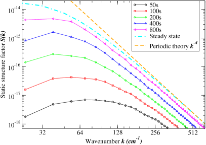
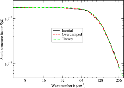
Figure 1: (Color online) (Left) Time evolution of the static structure factor $S(k;t)$ in the GRADFLEX experiment FractalDiffusion_Microgravity . The steady-state spectrum, studied in more detail in Section V in LLNS_Staggered , is also shown, and compared to the simple quasi-periodic theory (140). At smaller wavenumbers the steady-state fluctuations are damped due to confinement effects. (Right) Static structure factor $S(k)$ of concentration fluctuations in a binary liquid mixture subjected to a steady temperature gradient SoretDiffusion_Croccolo . In order to account for spatial discretization artifacts, on the $x$ axes we show the modified wave number $\sin\left(k\Delta x/2\right)/\left(\Delta x/2\right)$ LLNS_Staggered . The theory (140) is shown for comparison.

In the left panel of Fig. 1 we show the static structure factor as a function of time, along with the steady state asymptotic value. We observe that it takes a long time, on the time scale of the macroscopic diffusive mixing, to actually establish the steady state. This is in contrast to experiments performed in gravity, where gravity accelerates the dynamics of the concentration fluctuations at the smaller wavenumbers, as seen in (142). This was used in Refs. GiantFluctuations_Theory ; GiantFluctuations_Cannell to construct a simple but approximate theory for the time evolution of the static structure factor during free diffusive mixing of two miscible liquids. Such a simple theory cannot be developed in microgravity because there is no separation of time scales between the dynamics of the mean and the dynamics of the fluctuations around the mean, and computer simulations become indispensable.

V.2 Giant Fluctuations in Earth Gravity

In this section we consider giant fluctuations in the presence of gravity. We model the experiments used in Ref. SoretDiffusion_Croccolo to measure the Soret and diffusion coefficients in binary mixtures using a setup similar to that in the GRADFLEX experiment described in the previous section. A notable difference is that the average concentration $\vartheta_{0}\approx 0.5$ is much larger than in the GRADFLEX setup, and only a small relative concentration difference is induced by an applied modest temperature gradient. We therefore approximate $c\left(1-c\right)\approx\vartheta_{0}\left(1-\vartheta_{0}\right)$ in (138), giving a constant mass Soret flux. In this example, because we want to accurately resolve the decay of the time correlation functions over several orders of magnitude, we perform two dimensional simulations. As we already explained, there is no difference between two and three dimensional simulations because of the simple one-dimensional geometry of the deterministic solution FluctHydroNonEq_Book .

By linearizing the inertial dynamics (137,138) and taking a spatio-temporal Fourier transform we can obtain an approximate theory for the spatio-temporal correlation functions for the concentration fluctuations. This straightforward analysis predicts that the static factor $S\left(k\right)$ continues to follow (140) if $\nu\gg\chi$, but the time correlation function, unlike the overdamped result (144), is found to be a sum of two modes

$$S(k,t)=S_{0}\exp\left(-\frac{t}{\tau_{1}}\right)+\left(S\left(k\right)-S_{0}\right)\exp\left(-\frac{t}{\tau_{2}}\right),$$ (144)

where we omit the long formula for $S_{0}$ and just quote the relaxation times

$$\tau_{1/2}^{-1}=\frac{1}{2}\left(\nu+\chi\right)k^{2}\pm\frac{1}{2}\,\sqrt{k^{4}\left(\nu-\chi\right)^{2}-4\beta gh}.$$

In the limit $\nu/\chi\rightarrow\infty$, we get the diffusive relaxation time (142) if we use the minus sign, $\tau_{\chi}^{-1}\approx\chi k^{2}$, and for the plus sign we get the viscous relaxation time

$$\tau_{\nu}^{-1}=\nu k^{2}\left[1-\frac{\beta gh}{\nu\chi k^{4}}\right]\approx\nu k^{2}.$$ (145)

where $\nu=\eta/\rho$.

Note however that the relaxation times become complex-valued for

$$k_{p}\lesssim\left(\frac{4\beta gh}{\nu^{2}}\right)^{\frac{1}{4}}=\left(4\frac{\chi}{\nu}\right)^{\frac{1}{4}}k_{c}=\sqrt{2}\,S_{c}^{-\frac{1}{4}}k_{c},$$

indicating the appearance of propagative rather than diffusive modes for small wavenumbers. Because of the fourth root power, for realistic values of $S_{c}\sim 10^{4}$, propagative modes appear at wavenumbers that are, in principle, observable in experiments via very low-angle light scattering and shadowgraph techniques, although, to our knowledge, experimental observation of propagative modes has only been reported for temperature fluctuations TemperatureGradient_Cannell . This shows that there is a qualitative difference between the inertial and overdamped dynamics in this example. This comes because of the lack of separation between the relaxation times associated with mass ($\tau_{\chi}$) and momentum diffusion ($\tau_{\nu}$) for wavenumbers $k\lesssim k_{p}$. In order to obtain accurate results over the whole range of wavenumbers observed in experiments, we need to account for the fluid inertia and integrate the system in time using Algorithm (1). For comparison we also numerically take the overdamped limit and use Algorithm (3) for the temporal integration.

In our simulations we use a grid of $128\times 128$ cells, with grid spacing $\Delta x=\Delta y=1/128$cm. This corresponds to thickness of the sample of $H=L=1\mbox{cm}$. The physical parameters correspond to the THN-C12 mixture studied in SoretDiffusion_Croccolo , $\rho=0.8407\,\mbox{g}/\mbox{cm}^{3}$, $\chi=6.21\cdot 10^{-6}\,\mbox{cm}^{2}/\mbox{s}$, $\nu=1.78\cdot 10^{-2}\,\mbox{cm}^{2}/\mbox{s}$, $T_{0}=300\,\mbox{K}$, $S_{T}=9.5\cdot 10^{-3}\,\mbox{K}^{-1}$, $\beta=0.27$, $g=981\,\mbox{cm}/\mbox{s}^{2},$ and the temperature difference across the sample is $\Delta T=40\,\mbox{K}$. To obtain the time-correlation functions we analyze a single run corresponding to $3,125\,\mbox{s}$ of physical time, skipping the initial $625\,\mbox{s}$. The time step used in both the inertial and overdamped integrators is $\Delta t=5\cdot 10^{-3}$s, giving a viscous Courant number $\nu\Delta t/\Delta x^{2}=1.5$. This means that the viscous dynamics is well-resolved by this small time step and there is no real benefit from using the overdamped equations. A larger time step cannot be used here even in the overdamped limit because the relaxation time (142) for the smallest wave number $k\approx 6.28\,\text{cm}^{-1}$ is $\tau=0.025\,\text{s}$, and therefore resolving the dynamics of the concentration requires a rather small time step.

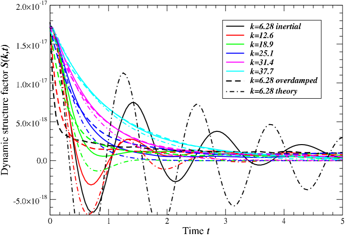
Figure 2: (Color online) Time correlation functions $S(k,t)$ of concentration fluctuations for concentration fluctuations in a binary liquid mixture subjected to a temperature gradient SoretDiffusion_Croccolo , for the first few wavenumbers (listed in the legend in $\mbox{cm}^{-1}$). Solid lines are obtained using the inertial equations, while dashed lines of the same color are obtained using the overdamped approximation. For the smallest two wavenumbers clear oscillations are observed indicating the appearance of propagative modes. These are not captured correctly in the overdamped approximation, and are only qualitatively described by the simple theory (144), shown with dashed-dotted lines.

In the right panel of Fig. 1 we show numerical results for the static structure factor $S(\boldsymbol{k})$, while in Fig. 2 we show results for the dynamic structure factor $S(\boldsymbol{k},t)$. While the static factor shows no difference between the inertial and overdamped integrators, the dynamic factor clearly shows the appearance of oscillations (propagative modes) for the smallest wavenumbers when inertia is accounted for. For comparison, in Fig. 2 we also plot the theory (144). We see a qualitative but not a quantitative agreement between the numerical results and the theory. This mismatch can be attributed to the effects of confinement by the two no-sip boundaries, which is not taken into account in the simple quasi-periodic theory used to derive (144). This effect becomes stronger the smaller the value of the dimensionless product $kH$ is. Constructing analytical theories in the presence of confinement and inertial effects is quite challenging and computer simulations are required to study these effects, which we will explore in more detail in future publications.

VI Conclusions

Continuing on our previous work DFDB , we constructed a general class of mixed explicit-implicit predictor-corrector schemes for integrating Langevin equations, and recommended two specific schemes that we previously proposed in DFDB in the context of additive-noise Langevin equations. The first is a fully explicit midpoint rule, and the second is a semi-implicit scheme in which some of the terms are treated using an implicit trapezoidal rule and the rest are treated using an explicit trapezoidal rule. Here we showed how to add stochastic forcing terms to these schemes that ensure the following key properties: the schemes are second-order weakly accurate for linearized Langevin equations, and they are weakly first-order accurate for multiplicative kinetic noise. In particular, we discussed how to obtain all of the required stochastic drift terms without evaluating derivatives, using random finite differences that give the required stochastic drift in expectation.

The key idea in our approach was to discretize the original nonlinear Langevin equations with sufficiently weak noise, and let the algorithm do the linearization for us, without us having to even write the linearized equations explicitly. This has numerous advantages over the alternative approach of splitting the variables into a deterministic mean plus fluctuations and then linearizing the equations manually. Firstly, the linearization needs to be done around an unknown time-dependent solution of the deterministic equations, which must itself be computed numerically in general. Secondly, the linearized equations typically have many more terms than the nonlinear equations, and do not obey conservation laws, leading to violation of conservation for the overall solution (mean+fluctuations). Lastly, our algorithms can, with care, also be used to integrate genuinely nonlinear Langevin equations, and thus numerically access the importance of terms neglected by linearization DiffusionRenormalization ; DiffusionJSTAT . Integrating the linearized equations to second-order weak accuracy proved to be relatively simple. Essentially, all that is required is to evaluate the noise amplitude in the corrector step at the correct value for the time-dependent deterministic solution, e.g., at the midpoint or end-point of the time step. In the general nonlinear setting, by contrast, obtaining second-order accuracy with derivative-free schemes is rather nontrivial WeakSecondOrder_RK .

We also proposed predictor-corrector schemes for integrating systems of Langevin equations containing a fast and a slow variable, in the limit of infinite separation of time scales. We limited our attention here to the simple but common case of the fast variable entering only linearly; the general case is much more subtle AdiabaticElimination_1 . Our predictor-corrector schemes discretize the original equations but without the time derivative term in the equation for the fast variable, giving an effective integrator for the overdamped equations without ever explicitly even writing the limiting dynamics. One way to think about our integrators is as applying a backward Euler method to the fast variable, since this method finds a steady state solution of the fast variable in the limit when the time step size is much larger than the internal time scale of the fast variable. An essential difficulty in the construction of integrators for the nonlinear overdamped equations is capturing the stochastic drift terms that arise due to the kinetic interpretation of the noise. We accomplished this goal by using a combination of implicit and explicit random finite differences.

The integrators proposed here handle fast-slow systems by taking the limit of infinite separation of variables to eliminate the fast variable. Such an asymptotic limit is often a good approximation, as we illustrated in the past when modeling diffusion in liquids DiffusionJSTAT , and also here by modeling the development of giant fluctuations in microgravity during the GRADFLEX experiment FractalDiffusion_Microgravity . However, we also studied here the dynamics of giant fluctuations in Earth gravity and found that the assumption of uniform separation of time scales between the fast velocity and slow concentration fails in practice for sufficiently small wavenumbers. In this paper, we resorted to integrating the original (inertial) equations using a sufficiently small time step. It remains an important challenge for the future to develop uniformly accurate temporal integrators that remain weakly first-order accurate even when there is incomplete separation of time scales, while still allowing the use of large time step sizes, on the time scale of the slow variable. Such integrators must likely rely on the linearity of the equation and exponential integrators SDEWeakExponential ; StochasticExponential ; StochasticImmersedBoundary for the fast variable. The key difficulty, which we hope to address in future work, is to correctly capture the effects of the fast velocity on the slow concentration that arise due to the nonlinear advective term $\boldsymbol{v}\cdot\boldsymbol{\nabla}c$ DiffusionJSTAT .

Appendix

Appendix A Accuracy for time dependent noise

In this appendix, we show that the scheme (29) successfully captures the time dependence of $\boldsymbol{K}$ in the equation (28) to second order. The general theory of weak accuracy for stochastic integrators is well-established and reviewed, for example, in Section 2.2 of MilsteinSDEBook . The key result is that, under certain assumptions, second-order weak accuracy is achieved if the first $5$ moments of the numerical increment $\Delta\boldsymbol{x}^{n}=\boldsymbol{x}^{n+1}-\boldsymbol{x}^{n}$ match the moments of the true increment $\boldsymbol{x}\left(n\Delta t+\Delta t\right)-\boldsymbol{x}\left(n\Delta t\right)$ with error no greater than $O\left(\Delta t^{3}\right)$. The time dependence of the noise amplitude only adds one additional term (beyond constant noise) that a second-order integrator must account for, which we find from the expansion

$$\int_{t_{n}}^{t_{n+1}}\boldsymbol{K}(s)\,d\boldsymbol{\mathcal{B}}(s)= \,\boldsymbol{K}(t_{n})\int_{t_{n}}^{t_{n+1}}\,d\boldsymbol{\mathcal{B}}(s)+\boldsymbol{\partial K}(t_{n})\int_{t_{n}}^{t_{n+1}}(s-t_{n})\,d\boldsymbol{\mathcal{B}}(s)$$ (146)

$$+\boldsymbol{\partial^{2}K}(t_{n})\int_{t_{n}}^{t_{n+1}}\frac{(s-t_{n})^{2}}{2}\,d\boldsymbol{\mathcal{B}}(s)+O\left(\Delta t^{7/2}\right).$$

Here $\boldsymbol{\partial K}$ indicates a time derivative of $\boldsymbol{K}$, and likewise $\boldsymbol{\partial^{2}K}$ indicates a second derivative in time. The first term in the second line is order $\Delta t^{5/2}$ and mean zero, so it will not affect second order weak accuracy. Likewise, terms which arise from the time dependence of $\boldsymbol{K}$ in the Taylor expansion of the deterministic part of (28) are all order greater than two and a half and mean zero. Therefore, the only additional expression which must be accounted for in the temporal integrator is the second term on the first line of equation (146). When matching increments for second order weak accuracy, this term appears only in the second moment of the increment, and only in the cross term with $\boldsymbol{K}(t_{n})\int_{t_{n}}^{t_{n+1}}d\boldsymbol{\mathcal{B}}(s)$,

$$E\left[\left(\boldsymbol{x}(t_{n+1})-\boldsymbol{x}(t_{n})\right)\left(\boldsymbol{x}(t_{n+1})-\boldsymbol{x}(t_{n})\right)^{\star}\right]= \ldots+\left((\boldsymbol{\partial K})\boldsymbol{K}^{\star}+\boldsymbol{K}(\boldsymbol{\partial K}){}^{\star}\right)\frac{\Delta t^{2}}{2}+O(\Delta t^{3})$$ (147)

where the terms that are present in the constant-noise case already appear in (16) in DFDB and are denoted with ellipses.

In order to maintain second order weak accuracy, the additional term involving $\boldsymbol{\partial K}$ in (147) is matched in the temporal integrator by the way in which the noise is evaluated in the corrector step of (29),

$$\boldsymbol{x}^{n+1}-\boldsymbol{x}^{n}= \ldots+\left((1-w_{7})\boldsymbol{K}^{n}+w_{7}\boldsymbol{K}^{(p)}\right)\left(\sqrt{w_{2}\Delta t}\,\boldsymbol{W}^{n,1}+\sqrt{(1-w_{2})\Delta t}\,\boldsymbol{W}^{n,2}\right),$$ (148)

where deterministic terms are denoted by elipses. Taylor expanding $\boldsymbol{K}^{(p)}$ in (148) gives the following two terms,

$$\boldsymbol{x}^{n+1}-\boldsymbol{x}^{n}= \ldots+\Delta t^{1/2}\,\boldsymbol{K}^{n}\left(\sqrt{w_{2}}\,\boldsymbol{W}^{n,1}+\sqrt{1-w_{2}}\,\boldsymbol{W}^{n,2}\right)$$

$$+\Delta t^{3/2}w_{2}w_{7}\boldsymbol{\partial K}\left(\sqrt{w_{2}}\,\boldsymbol{W}^{n,1}+\sqrt{1-w_{2}}\,\boldsymbol{W}^{n,2}\right)+O(\Delta t^{5/2}).$$ (149)

The terms on the right hand side create the correct cross term in the second moment of the increment as long as $w_{2}w_{7}=1/2$. Therefore, scheme (29) is second order weakly accurate even for time-dependent additive noise.

Appendix B Second-order weak integrators for linearized fluctuating hydrodynamics

Here we show that the scheme (40) is second order accurate for the linearized equations (26,27). For the scheme to be weakly second order accurate, we need the difference between the first five moments of the discrete and continuous increments for the composite variable $\left(\bar{\boldsymbol{x}}(t),\,\delta\boldsymbol{x}(t)\right)$ to be $O\left(\Delta t^{3}\right)$ MilsteinSDEBook . The scheme (41) for the mean is deterministic and standard Taylor series analysis shows that it is second-order accurate. Furthermore, because $\boldsymbol{\bar{x}}$ is deterministic, there are no cross-correlations between increments of $\bar{\boldsymbol{x}}$ and $\delta\boldsymbol{x}$, and therefore moments that involve both variables are guaranteed to match to the same order as the increments in $\delta\boldsymbol{x}$.

In order to examine the moments of the increment in $\delta\boldsymbol{x}$, let us re-write equation (27) in differential and index notation,

$$d(\delta x_{i})= M_{ij}\left(\bar{x}\left(t\right)\right)\delta x_{j}\,dt+K_{ij}\left(\bar{x}\left(t\right)\right)d\mathcal{B}_{j}\left(t\right),$$ (150)

where as before $M_{ij}=H_{ij}+\partial_{j}(H_{ik})\bar{x}_{k}+\partial_{j}(h_{i})$, giving

$$\partial_{k}\left(M_{ij}\right)=\partial_{k}\left(H_{ij}\right)+\partial_{kj}\left(H_{il}\right)\bar{x}_{l}+\partial_{j}\left(H_{ik}\right)+\partial_{jk}\left(h_{i}\right).$$

Using the deterministic equation

$$d\bar{x}_{k}/dt=H_{kl}\bar{x}_{l}+h_{k},$$

it can be shown that over a time interval $\Delta t=t^{n+1}-t^{n}$, the random variable $\delta x_{i}$ has the following continuous increment,

$$\Delta\left(\delta x_{i}\right)=\delta x_{i}(t^{\prime})-\delta x_{i}\left(t\right)= \Delta t\,M_{ij}\delta x_{j}+K_{ij}\int_{t^{n}}^{t^{n+1}}d\mathcal{B}_{j}(s)$$ (151)

$$+\frac{\Delta t^{2}}{2}\partial_{k}\left(M_{ij}\right)\delta x_{j}\left(\frac{d\bar{x}_{k}}{dt}\right)+\frac{\Delta t^{2}}{2}M_{ij}M_{jk}\delta x_{k}$$

$$+\partial_{k}\left(K_{ij}\right)\left(\frac{d\bar{x}_{k}}{dt}\right)\int_{t^{n}}^{t^{n+1}}(s-t)\,d\mathcal{B}_{j}(s)+M_{ij}K_{jk}\int_{t^{n}}^{t^{n+1}}\int_{t}^{s}\,d\mathcal{B}_{k}(r)\,ds+O(\Delta t^{5/2})$$

where in this equation and in the following, $d\bar{x}_{k}/dt$, as well as $\boldsymbol{M},\,\boldsymbol{H},\,\boldsymbol{K}$, and $\boldsymbol{h}$ and their derivatives, are all evaluated at the beginning of the time step.

In order to compare this to the discrete increment, we need to perform a Taylor expansion of every term in equation (43) that is not already evaluated at $\bar{\boldsymbol{x}}^{n}$. These expansions never need to include terms of higher order than $\Delta t^{3/2}$, considering that all terms in (43) are already at least order $\Delta t^{1/2}$ (any term that is $O(\Delta t^{5/2})$ is mean zero and thus irrelevant). Additionally, the only term to be expanded which is order $\Delta t^{1/2}$ before expansion is the stochastic term $w_{7}K_{ij}^{p}\left(\sqrt{w_{2}\Delta t}\,W_{j}^{1,n}+\sqrt{(1-w_{2})\Delta t}\,W_{j}^{2,n}\right)$, which depends only on the deterministic variable $\bar{\boldsymbol{x}}$. Thus an expansion of $K_{ij}^{p}$ to order $\Delta t^{3/2}$ only includes first order terms. All other terms in (43) to be expanded are of order $\Delta t$ or greater before expansion, so in fact we only need to consider first order expansions for all quantities evaluated at $\bar{\boldsymbol{x}}^{p}$ or $\bar{\boldsymbol{x}}^{n+1}$ in the discrete increment.

For $\delta\boldsymbol{x},$ we expand the update (42,43) to first order, substitute the result in the corrector update (43), and Taylor expand terms involving $\boldsymbol{M},\,\boldsymbol{H},\,\boldsymbol{K}$, and $\boldsymbol{h}$ evaluated at a point other than $\bar{\boldsymbol{x}}^{n}$ to first order. Note that both options for the handling of the explicit term in (40) yield the same increment to second order. After performing these expansions and collecting some terms, we get the final discrete increment to second order,

$$\Delta\left(\delta x_{i}\right)=\delta x_{i}^{n+1}-\delta x_{i}^{n}= \Delta t\,M_{ij}\delta x_{j}+\Delta t^{1/2}K_{ij}\left(\sqrt{w_{2}}W_{j}^{1}+\sqrt{(1-w_{2})}W_{j}^{2}\right)$$

$$+\Delta t^{2}\delta x_{j}\left(H_{km}\bar{x}_{m}+h_{k}\right)\times$$ (152)

$$\;\left(\left(w_{2}w_{3}+w_{2}w_{4}\right)\left(\partial_{k}(H_{ij})+\partial_{kj}(H_{il})\bar{x}_{l}\right)+w_{2}w_{6}\partial_{kj}\left(h_{i}\right)+\left(w_{2}w_{3}+w_{4}+w_{5}\right)\partial_{j}(H_{ik})\right)$$

$$+\Delta t^{2}\left(\left(w_{2}w_{3}+w_{4}+w_{5}\right)H_{ij}+\left(w_{2}w_{3}+w_{2}w_{4}\right)\partial_{j}(H_{il})\bar{x}_{l}+w_{2}w_{6}\partial_{j}(h_{i})\right)M_{jk}\delta x_{k}$$

$$+\Delta t^{3/2}w_{2}w_{7}\partial_{k}(K_{ij})\left(H_{kl}\bar{x}_{l}+h_{k}\right)\left(\sqrt{w_{2}}\,W_{j}^{1}+\sqrt{1-w_{2}}\,W_{j}^{2}\right)$$

$$+\Delta t^{3/2}\left(\left(w_{3}+w_{4}+w_{5}\right)\sqrt{w_{2}}\,W_{k}^{1}+\left(w_{4}+w_{5}\right)\sqrt{1-w_{2}}\,W_{k}^{2}\right)H_{ij}K_{jk}$$

$$+\Delta t^{3/2}\left(w_{3}+w_{4}\right)\sqrt{w_{2}}\,\partial_{k}(H_{ij})\bar{x}_{k}K_{jl}W_{l}^{1}$$

$$+\Delta t^{3/2}w_{6}\sqrt{w_{2}}\partial_{k}(h_{i})K_{kl}W_{l}^{1}+O(\Delta t^{5/2}),$$

where we have omitted bars since all quantities and derivatives are evaluated at $\bar{\boldsymbol{x}}^{n}$.

The first moment includes only the deterministic terms, and making use of the relations (30) confirms that they match the continuous increment with error $O(\Delta t^{3})$. The second moment is more complicated due to the cross correlations that arise from the stochastic terms, but after some algebra and again making use of (30), we see that the increments match to the correct order. The third moment only contains the second order products of the first two terms in the right hand side of (152). The fourth moment contains only the fourth moment of the lowest order stochastic term, $K_{ij}\left(\sqrt{w_{2}\Delta t}W_{j}^{1}+\sqrt{(1-w_{2})\Delta t}W_{j}^{2}\right)$. The fifth moment is zero for both increments. All of these moments match with error no greater than order $\Delta t^{3}$, and hence the scheme (43) is second order accurate.

Appendix C Kinetic noise in fast-slow system

In this section, we show that the schemes (65, 89) and (101, 106, 126) from section III produce the correct thermal drift arising from the kinetic interpretation of the overdamped limit (III). It is useful to consider the drift split into the following pieces,

$$\left[\partial_{\boldsymbol{x}}\cdot\left(\boldsymbol{A}+\boldsymbol{B}\boldsymbol{C}^{-1}\boldsymbol{B}^{\star}\right)\right]_{i}=\partial_{j}\left(A_{ij}+B_{ik}C_{kl}^{-1}B_{jl}\right)= \partial_{j}\left(A_{ik}^{\frac{1}{2}}A_{jk}^{\frac{1}{2}}\right)+\partial_{j}\left(B_{ik}C_{kl}^{-1}\right)B_{jl}+B_{ik}C_{kl}^{-1}\partial_{j}\left(B_{jl}\right),$$ (153)

where we have rewritten $\boldsymbol{A}^{\frac{1}{2}}\equiv\boldsymbol{A}_{\frac{1}{2}}$and $\boldsymbol{C}^{\frac{1}{2}}\equiv\boldsymbol{C}_{\frac{1}{2}}$ in order to simplify the notation. The first term on the right hand side of equation (153) can be split into

$$\partial_{j}\left(A_{ik}^{\frac{1}{2}}A_{jk}^{\frac{1}{2}}\right)= \partial_{j}\left(A_{ik}^{\frac{1}{2}}\right)A_{jk}^{\frac{1}{2}}+A_{ik}^{\frac{1}{2}}\partial_{j}\left(A_{jk}^{\frac{1}{2}}\right),$$ (154)

and the second term on the right hand side of equation (153) can be rewritten as

$$\partial_{j}\left(B_{ik}C_{kl}^{-1}\right)B_{jl}= \partial_{j}\left(B_{ik}C_{kl}^{-1}\right)B_{jn}\delta_{nl}=\partial_{j}\left(B_{ik}C_{kl}^{-1}\right)B_{jn}\left(C_{np}^{-1}C_{pm}^{\frac{1}{2}}C_{lm}^{\frac{1}{2}}\right)$$ (155)

$$= \partial_{j}\left(B_{ik}C_{kl}^{-1}C_{lm}^{\frac{1}{2}}\right)B_{jn}C_{np}^{-1}C_{pm}^{\frac{1}{2}}-B_{ik}C_{kl}^{-1}\partial_{j}\left(C_{lm}^{\frac{1}{2}}\right)B_{jn}C_{np}^{-1}C_{pm}^{\frac{1}{2}}.$$

Making use of relations (154, 155) gives the following form of the entire drift

$$\partial_{j}\left(A_{ij}+B_{ik}C_{kl}^{-1}B_{jl}\right)= \left(\partial_{j}\left(A_{ik}^{\frac{1}{2}}\right)A_{jk}^{\frac{1}{2}}+\partial_{j}\left(B_{ik}C_{kl}^{-1}C_{lm}^{\frac{1}{2}}\right)B_{jn}C_{np}^{-1}C_{pm}^{\frac{1}{2}}\right)$$ (156)

$$+ \left(A_{ik}^{\frac{1}{2}}\partial_{j}\left(A_{jk}^{\frac{1}{2}}\right)+B_{ik}C_{kl}^{-1}\partial_{j}\left(B_{jl}\right)-B_{ik}C_{kl}^{-1}\partial_{j}\left(C_{lm}^{\frac{1}{2}}\right)B_{jn}C_{np}^{-1}C_{pm}^{\frac{1}{2}}\right),$$

The first line of equation (156) is generated by the evaluation of the noise in the corrector step, and the second line will be approximated using RFD terms.

Both the implicit trapezoidal and explicit midpoint schemes have the following noise term in the corrector step,

$$x_{i}^{n+1}-x_{i}^{n}= \ldots+\sqrt{k_{B}T\Delta t}\left((1-w_{7})A_{ik}^{\frac{1}{2},n}+w_{7}A_{ik}^{\frac{1}{2},p}\right)\left(\sqrt{w_{2}}W_{k}^{n,1,x}+\sqrt{1-w_{2}}W_{k}^{n,2,x}\right)$$

$$+\sqrt{k_{B}T\Delta t}\left((1-w_{7})\left(B_{ik}C_{kl}^{-1}C_{lm}^{\frac{1}{2}}\right)^{n}+w_{7}\left(B_{ik}C_{kl}^{-1}C_{lm}^{\frac{1}{2}}\right)^{p}\right)\left(\sqrt{w_{2}}W_{m}^{n,1,y}+\sqrt{1-w_{2}}W_{m}^{n,2,y}\right),$$ (157)

which after Taylor expanding operators evaluated at the predictor to $O\left(\sqrt{\Delta t}\right)$ and taking expectation with respect to $\boldsymbol{W}^{x}$ and $\boldsymbol{W}^{y}$, becomes

$$\langle x_{i}^{n+1}-x_{i}^{n}\rangle= \ldots+\left(2w_{2}w_{7}\right)\Delta t\,k_{B}T\left(\partial_{j}\left(A_{ik}^{\frac{1}{2}}\right)A_{jk}^{\frac{1}{2}}+\partial_{j}\left(B_{ik}C_{kl}^{-1}C_{lm}^{\frac{1}{2}}\right)B_{jn}C_{np}^{-1}C_{pq}^{\frac{1}{2}}\right)+O\left(\Delta t^{2}\right).$$ (158)

The term on the right-hand side of (158) thus gives the first line of the drift (156) when $w_{2}w_{7}=1/2$.

The RFD terms from both schemes give the following additional increment in $\boldsymbol{x}$,

$$x_{i}^{n+1}-x_{i}^{n}= \ldots+\frac{\Delta t\,k_{B}T}{\delta}A_{ik}^{\frac{1}{2}}\left(\boldsymbol{A}_{jk}^{\frac{1}{2}}(\boldsymbol{x}^{n}+\delta\widetilde{\boldsymbol{W}})-A_{jk}^{\frac{1}{2}}(\boldsymbol{x}^{n})\right)\widetilde{W}_{j}^{A}$$

$$+\frac{\Delta t\,k_{B}T}{\delta}\left(B_{ik}C_{kl}^{-1}\right)^{p}\left(B_{kl}(\boldsymbol{x}^{n}+\delta\widetilde{\boldsymbol{W}})-B_{kl}(\boldsymbol{x}^{n})\right)\widetilde{W}_{m}^{A},$$ (159)

$$-\frac{\Delta t\,k_{B}T}{\delta}\left(B_{ik}C_{kl}^{-1}\right)^{p}\left(C_{lm}^{\frac{1}{2}}\left(\boldsymbol{x}^{n}+\delta\boldsymbol{B}\boldsymbol{C}^{-1}\boldsymbol{C}^{\frac{1}{2}}\widetilde{\boldsymbol{W}}^{C}\right)\,-C_{lm}^{\frac{1}{2}}(\boldsymbol{x}^{n})\right)\widetilde{W}_{m}^{C}$$ (160)

where all terms except for the RFD term have been omitted for this analysis. Expanding terms not evaluated at $\boldsymbol{x}^{n}$ to $O(\delta^{2})$ in (159), and taking expectation with respect to $\widetilde{\boldsymbol{W}}^{A}$ and $\widetilde{\boldsymbol{W}}^{C}$ gives

$$\langle x_{i}^{n+1}-x_{i}^{n}\rangle= \ldots+\Delta t\left(k_{B}T\right)\left(A_{ik}^{\frac{1}{2}}\partial_{j}\left(A_{jk}^{\frac{1}{2}}\right)+B_{ik}C_{kl}^{-1}\partial_{j}\left(B_{jl}\right)-B_{ik}C_{kl}^{-1}\partial_{j}\left(C_{lm}^{\frac{1}{2}}\right)B_{jn}C_{np}^{-1}C_{pm}^{\frac{1}{2}}\right),$$

which corresponds to the drift term in the second line of equation (156). Together, the RFD terms in (159) and the noise terms in (157) create the entire thermal drift from (III), demonstrating that our schemes are first order accurate for the fully nonlinear kinetic equations.

References

• (1) L.D. Landau and E.M. Lifshitz. Fluid Mechanics, volume 6 of Course of Theoretical Physics. Pergamon Press, Oxford, England, 1959.
• (2) R.F. Fox and G.E. Uhlenbeck. Contributions to Non-Equilibrium Thermodynamics. I. Theory of Hydrodynamical Fluctuations. Physics of Fluids, 13:1893, 1970.
• (3) J. M. O. De Zarate and J. V. Sengers. Hydrodynamic fluctuations in fluids and fluid mixtures. Elsevier Science Ltd, 2006.
• (4) A. Vailati and M. Giglio. Giant fluctuations in a free diffusion process. Nature, 390(6657):262–265, 1997.
• (5) B. Davidovitch, E. Moro, and H.A. Stone. Spreading of viscous fluid drops on a solid substrate assisted by thermal fluctuations. Phys. Rev. letters, 95(24):244505, 2005.
• (6) A. Vailati, R. Cerbino, S. Mazzoni, C. J. Takacs, D. S. Cannell, and M. Giglio. Fractal fronts of diffusion in microgravity. Nature Communications, 2:290, 2011.
• (7) A. Donev, T. G. Fai, and E. Vanden-Eijnden. A reversible mesoscopic model of diffusion in liquids: from giant fluctuations to Fick’s law. Journal of Statistical Mechanics: Theory and Experiment, 2014(4):P04004, 2014.
• (8) D. Bedeaux, I. Pagonabarraga, J.M.O. de Zárate, J.V Sengers, and S. Kjelstrup. Mesoscopic non-equilibrium thermodynamics of non-isothermal reaction-diffusion. Phys. Chem. Chem. Phys., 12(39):12780–12793, 2010.
• (9) R.V. Kohn, M.G. Reznikoff, and E. Vanden-Eijnden. Magnetic elements at finite temperature and large deviation theory. Journal of nonlinear science, 15(4):223–253, 2005.
• (10) J. L. Lebowitz, E. Presutti, and H. Spohn. Microscopic models of hydrodynamic behavior. J. Stat. Phys., 51(5):841–862, 1988.
• (11) P. Español. Stochastic differential equations for non-linear hydrodynamics. Physica A, 248(1-2):77–96, 1998.
• (12) P. Español, J.G. Anero, and I. Zúñiga. Microscopic derivation of discrete hydrodynamics. J. Chem. Phys., 131:244117, 2009.
• (13) H. C. Öttinger. Beyond equilibrium thermodynamics. Wiley Online Library, 2005.
• (14) S. Delong, B. E. Griffith, E. Vanden-Eijnden, and A. Donev. Temporal Integrators for Fluctuating Hydrodynamics. Phys. Rev. E, 87(3):033302, 2013.
• (15) P. Español and I. Zúñiga. On the definition of discrete hydrodynamic variables. J. Chem. Phys, 131:164106, 2009.
• (16) A. Donev and E. Vanden-Eijnden. Dynamic Density Functional Theory with hydrodynamic interactions and fluctuations. J. Chem. Phys., 140(23), 2014.
• (17) Martin Hairer. Introduction to regularity structures. arXiv preprint arXiv:1401.3014, 2014.
• (18) Giambattista Giacomin, Joel L Lebowitz, and Errico Presutti. Deterministic and stochastic hydrodynamic equations arising from simple microscopic model systems. In Stochastic Partial Differential Equations: Six Perspectives, number 64 in Mathematical Surveys and Monographs, page 107. American Mathematical Soc., 1999.
• (19) S. R. S. Varadhan. The complex story of simple exclusion. In Ito’s stochastic calculus and probability theory, pages 385–400. Springer, 1996.
• (20) C Kipnis, S Olla, and SRS Varadhan. Hydrodynamics and large deviation for simple exclusion processes. Communications on Pure and Applied Mathematics, 42(2):115–137, 1989.
• (21) S.R.S. Varadhan. Scaling limits for interacting diffusions. Communications in mathematical physics, 135(2):313–353, 1991.
• (22) A Abdulle, G Vilmart, and K Zygalakis. Weak second order explicit stabilized methods for stiff stochastic differential equations. SIAM J. Sci. Comput., 35(4):A1792–A1814, 2013.
• (23) S. Delong, F. Balboa Usabiaga, R. Delgado-Buscalioni, B. E. Griffith, and A. Donev. Brownian Dynamics without Green’s Functions. J. Chem. Phys., 140(13):134110, 2014.
• (24) A. J. Nonaka, Y. Sun, J. B. Bell, and A. Donev. Low Mach Number Fluctuating Hydrodynamics of Binary Liquid Mixtures. Submitted to CAMCOS, ArXiv preprint 1410.2300, 2015.
• (25) H. Grabert. Projection operator techniques in nonequilibrium statistical mechanics. Springer-Verlag, 1982.
• (26) J.D. Ramshaw and K. Lindenberg. Augmented Langevin description of multiplicative noise and nonlinear dissipation in Hamiltonian systems. J. Stat. Phys, 45(1):295–307, 1986.
• (27) M. Hütter and H.C. Öttinger. Fluctuation-dissipation theorem, kinetic stochastic integral and efficient simulations. J. Chem. Soc., Faraday Trans., 94(10):1403–1405, 1998.
• (28) G. C. Papanicolaou. Some probabilistic problems and methods in singular perturbations. Rocky Mountain J. Math, 6(4):653–674, 1976.
• (29) Grigorios A Pavliotis and Andrew M Stuart. Multiscale methods: averaging and homogenization, volume 53. Springer, 2008.
• (30) M. Fixman. Simulation of polymer dynamics. I. General theory. J. Chem. Phys., 69:1527, 1978.
• (31) David S Dean. Langevin equation for the density of a system of interacting langevin processes. Journal of Physics A: Mathematical and General, 29(24):L613, 1996.
• (32) A. Donev, A. J. Nonaka, Y. Sun, T. G. Fai, A. L. Garcia, and J. B. Bell. Low Mach Number Fluctuating Hydrodynamics of Diffusively Mixing Fluids. Communications in Applied Mathematics and Computational Science, 9(1):47–105, 2014.
• (33) A. Oprisan and A. Leilani Payne. Dynamic shadowgraph experiments and image processing techniques for investigating non-equilibrium fluctuations during free diffusion in nanocolloids. Optics Communications, 290:100–106, 2012.
• (34) F. Croccolo, H. Bataller, and F. Scheffold. A light scattering study of non equilibrium fluctuations in liquid mixtures to measure the Soret and mass diffusion coefficient. J. Chem. Phys., 137:234202, 2012.
• (35) F. Balboa Usabiaga, J. B. Bell, R. Delgado-Buscalioni, A. Donev, T. G. Fai, B. E. Griffith, and C. S. Peskin. Staggered Schemes for Fluctuating Hydrodynamics. SIAM J. Multiscale Modeling and Simulation, 10(4):1369–1408, 2012.
• (36) F. Croccolo, D. Brogioli, A. Vailati, M. Giglio, and D. S. Cannell. Nondiffusive decay of gradient-driven fluctuations in a free-diffusion process. Phys. Rev. E, 76(4):041112, 2007.
• (37) G. Da Prato. Kolmogorov equations for stochastic PDEs. Birkhauser, 2004.
• (38) C. W. Gardiner and M. L. Steyn-Ross. Adiabatic elimination in stochastic systems. I-III. Phys. Rev. A, 29:2814–2844, 1984.
• (39) RZ Khasminskii. Principle of averaging for parabolic and elliptic differential equations and for markov processes with small diffusion. Theory of Probability & Its Applications, 8(1):1–21, 1963.
• (40) Thomas G Kurtz. A limit theorem for perturbed operator semigroups with applications to random evolutions. Journal of Functional Analysis, 12(1):55–67, 1973.
• (41) B.E. Griffith, R.D. Hornung, D.M. McQueen, and C.S. Peskin. An adaptive, formally second order accurate version of the immersed boundary method. J. Comput. Phys., 223(1):10–49, 2007. Software available at http://ibamr.googlecode.com.
• (42) M. Cai, A. J. Nonaka, J. B. Bell, B. E. Griffith, and A. Donev. Efficient Variable-Coefficient Finite-Volume Stokes Solvers. 16(5):1263–1297, 2014. Comm. in Comp. Phys. (CiCP).
• (43) Jose Maria Ortiz de Zarate, Jose Antonio Fornes, and Jan V. Sengers. Long-wavelength nonequilibrium concentration fluctuations induced by the Soret effect. Phys. Rev. E, 74:046305, Oct 2006.
• (44) W. E, W. Ren, and E. Vanden-Eijnden. A general strategy for designing seamless multiscale methods. J. Comp. Phys., 228(15):5437–5453, 2009.
• (45) A. Vailati and M. Giglio. Nonequilibrium fluctuations in time-dependent diffusion processes. Phys. Rev. E, 58(4):4361–4371, 1998.
• (46) C. J. Takacs, G. Nikolaenko, and D. S. Cannell. Dynamics of long-wavelength fluctuations in a fluid layer heated from above. Phys. Rev. Lett., 100(23):234502, 2008.
• (47) A. Donev, A. L. Garcia, Anton de la Fuente, and J. B. Bell. Enhancement of Diffusive Transport by Nonequilibrium Thermal Fluctuations. J. of Statistical Mechanics: Theory and Experiment, 2011:P06014, 2011.
• (48) C.M. Mora. Weak exponential schemes for stochastic differential equations with additive noise. IMA journal of numerical analysis, 25(3):486–506, 2005.
• (49) Gabriel J Lord and Antoine Tambue. Stochastic exponential integrators for the finite element discretization of spdes for multiplicative and additive noise. IMA J Numer Anal, 33(2):515–543, 2013.
• (50) P. J. Atzberger, P. R. Kramer, and C. S. Peskin. A stochastic immersed boundary method for fluid-structure dynamics at microscopic length scales. J. Comp. Phys., 224:1255–1292, 2007.
• (51) G.N. Milstein and M.V. Tretyakov. Stochastic numerics for mathematical physics. Springer, 2004.