Sequential Design with Mutual Information for Computer Experiments (MICE): Emulation of a Tsunami Model

Joakim Beck Department of Statistical Science, University College London, London, UK. (joakim.beck@ucl.ac.uk)    Serge Guillas Department of Statistical Science, University College London, London, UK. (s.guillas@ucl.ac.uk)
Abstract

Computer simulators can be computationally intensive to run over a large number of input values, as required for optimization and various uncertainty quantification tasks. The standard paradigm for the design and analysis of computer experiments is to employ Gaussian random fields to model computer simulators. Gaussian process models are trained on input-output data obtained from simulation runs at various input values. Following this approach, we propose a sequential design algorithm, MICE (Mutual Information for Computer Experiments), that adaptively selects the input values at which to run the computer simulator, in order to maximize the expected information gain (mutual information) over the input space. The superior computational efficiency of the MICE algorithm compared to other algorithms is demonstrated by test functions, and a tsunami simulator with overall gains of up to 20% in that case.

1 Introduction

Computer experiments are widely employed to study physical processes [26, 31], and involve running a computer simulator which mimics the physical process at various input values. When the computer simulator is computationally expensive to run, say, minutes, hours, or even days, often on a high performance cluster, only a limited number of simulation runs can be afforded, making the planning of such experiments even more important. Surrogate models, also known as emulators, are often used as means for designing and analyzing computer experiments [26]. Emulators are statistical models that have been used to approximate the input-output behavior of computer simulators for making probabilistic predictions. In this setting, we want to find a design of computer experiments that with minimal computational effort leads to a surrogate model with a good overall fit. We restrict our attention to deterministic computer simulators with a scalar output. In design of experiments it is customary to use space-filling designs [31], such as uniform designs, multi-layer designs, maximin(Mm)- and minimax(mM)-distance designs, and Latin hypercube designs (LHD). Space-filling designs treat all regions of the design space as equally important, but are “one shot” designs that may waste computations over some unnecessary regions of the input space. A variety of adaptive designs have been proposed which can take advantage of information collected during the experimental design process [20, 26], typically in the form of input-output data from simulation runs. Some classical adaptive design criteria are the Maximum Mean Squared Prediction Error (MMSPE), the Integrated MSPE (IMSPE), and the entropy criterion (see, e.g., [25]).

We adopt the Design and Analysis of Computer Experiments (DACE) framework proposed in the seminal paper of Sacks et al. [25], within which the computer simulator output is modeled as a realization of a random field, typically assumed Gaussian. When given a set of input-output data, the Best Unbiased Linear Predictor (BLUP), and the associated mean squared prediction error (MSPE), for the random field can be expressed in closed forms [25, 26]. Moreover, when the random field is Gaussian, the resulting BLUP is a so-called Gaussian process (GP) emulator. GP emulators are routinely applied to handle computationally intensive computer simulators in the fields of simulation [26], global optimization [16], and uncertainty quantification [3, 27], among others. Applications include CFD simulation of a rocket booster [12], and climate simulation [5]. By using the GP approach a range of statistical design criteria can be estimated directly, see [5, 29]. Finding an optimal design is usually computationally very intensive, except for relatively small designs. A way to circumvent the issue is to consider sequential designs [5, 12, 20]. In a sequential design, points are systematically chosen, often one at a time. Sequential designs are generally not optimal, but often very effective in practice. An algorithm is called adaptive if it updates its behavior to new data. Two popular sequential designs are Active Learning MacKay (ALM), and Active Learning Cohn (ALC). ALC tends to have better overall predictive performance but involves a higher computational cost [12].

In this work we propose a new sequential algorithm, called MICE (Mutual Information for Computer Experiments), which is based on the information theoretic mutual information criterion, where the objective of maximizing the information a design provides about the other input values, as suggested by Caselton and Zidek [4]. Mutual information is a measure of the information contained in one random variable about another [7]. Krause et al. [18] later proposed a sequential mutual information (MI) algorithm for sensor placement, which sequentially maximizes the mutual information between a GP over the chosen sensor locations and another GP over the locations which have not yet been selected. The MICE criterion is a modified version of the MI criterion in [18], where an extra parameter is introduced to improve robustness. This modification is critical when high dimensional spaces are considered. We demonstrate by numerical examples that MICE balances well prediction accuracy and computational complexity. We are particularly interested in deterministic computer simulation experiments with more than just a few input variables.

The article is organized as follows. Section 2 reviews Gaussian process modeling for prediction, and present some popular sequential design algorithms within the DACE framework. In Section 2.2, a mutual information based design criterion is proposed for computer experiments. The MI algorithm is described in Section 3.1, and a practical limitation is shown in Section 3.1.2. Section 3.2 presents the MICE algorithm and some theoretical results. Section 4 details the computational costs associated with the different sequential design algorithms. A numerical comparison of MICE with other methods is provided for a few standard test functions, in lieu of computer simulators, in Section 5, and for a tsunami simulator that solves nonlinear shallow water equations in Section 6. Critically, we examine accuracy versus computational cost, as some algorithms can be quite time consuming. Section 7 summarizes our conclusions. Proofs of theorems are in the appendix.

2 Gaussian process modeling for prediction

We here follow the approach proposed by Sacks et al. [25], where a deterministic computer simulator y(𝒙):𝒳p:𝑦𝒙𝒳superscript𝑝y({\boldsymbol{x}}):{\mathcal{X}}\subseteq\mathbb{R}^{p}\to\mathbb{R} is treated as a random function, Y(𝒙)𝑌𝒙Y({\boldsymbol{x}}), 𝒙𝒳𝒙𝒳{\boldsymbol{x}}\in{\mathcal{X}}, except at the points where the simulator output is known. More specifically, Y(𝒙)𝑌𝒙Y({\boldsymbol{x}}) is modeled as a random field with E(Y2(𝒙))<𝐸superscript𝑌2𝒙E\left(Y^{2}({\boldsymbol{x}})\right)<\infty given a set of training data, which consists of n𝑛n input-output pairs (𝑿,𝒚)𝑿𝒚({\boldsymbol{X}},{\boldsymbol{y}}), where 𝑿=(𝒙j)j=1n𝑿subscriptsuperscriptsubscript𝒙𝑗𝑛𝑗1{\boldsymbol{X}}=\left({\boldsymbol{x}}_{j}\right)^{n}_{j=1}, 𝒚=(yj)j=1n𝒚subscriptsuperscriptsubscript𝑦𝑗𝑛𝑗1{\boldsymbol{y}}=\left(y_{j}\right)^{n}_{j=1}, and yj=y(𝒙j)subscript𝑦𝑗𝑦subscript𝒙𝑗y_{j}=y({\boldsymbol{x}}_{j}).

The aim is to determine a random process that can describe the set of data sufficiently well. It is customary that the mean E[Y(𝒙)]E𝑌𝒙\operatorname{E}[Y({\boldsymbol{x}})] takes the form 𝒉T(𝒙)𝜷superscript𝒉𝑇𝒙𝜷{\boldsymbol{h}}^{T}({\boldsymbol{x}}){\boldsymbol{\beta}}, that is, a linear combination of q𝑞q regressors 𝒉(𝒙):𝒳q:𝒉𝒙𝒳superscript𝑞{\boldsymbol{h}}({\boldsymbol{x}}):{\mathcal{X}}\to\mathbb{R}^{q} with coefficients 𝜷q𝜷superscript𝑞{\boldsymbol{\beta}}\in\mathbb{R}^{q}. In practice, a fixed constant, or a linear regression model, tends to perform well. The covariance Cov(Y(𝒙),Y(𝒙))Cov𝑌𝒙𝑌superscript𝒙\operatorname{Cov}(Y({\boldsymbol{x}}),Y({\boldsymbol{x}}^{\prime})), for 𝒙,𝒙𝒳𝒙superscript𝒙𝒳{\boldsymbol{x}},{\boldsymbol{x}}^{\prime}\in{\mathcal{X}}, is written in the form Σ(𝒙,𝒙;σ2)=σ2K(𝒙,𝒙)Σ𝒙superscript𝒙superscript𝜎2superscript𝜎2𝐾𝒙superscript𝒙\Sigma({\boldsymbol{x}},{\boldsymbol{x}}^{\prime};\sigma^{2})=\sigma^{2}K({\boldsymbol{x}},{\boldsymbol{x}}^{\prime}), where σ2(>0)annotatedsuperscript𝜎2absent0\sigma^{2}(>0) is a scale parameter (often called the process variance) and K(𝒙,𝒙)𝐾𝒙superscript𝒙K({\boldsymbol{x}},{\boldsymbol{x}}^{\prime}) is the correlation function. The correlation function is often expressed as a product of stationary, one-dimensional correlation functions. One such choice is the squared-exponential (SE) correlation [23]:

K(𝒙,𝒙;𝝃)=i=1pexp((xixi)22i2),𝐾𝒙superscript𝒙𝝃superscriptsubscriptproduct𝑖1𝑝superscriptsubscript𝑥𝑖superscriptsubscript𝑥𝑖22superscriptsubscript𝑖2K({\boldsymbol{x}},{\boldsymbol{x}}^{\prime};{\boldsymbol{\xi}})=\prod_{i=1}^{p}\exp\left(\frac{-(x_{i}-x_{i}^{\prime})^{2}}{2\ell_{i}^{2}}\right), (1)

where 𝝃=(1,2,,p)T+p𝝃superscriptsubscript1subscript2subscript𝑝𝑇subscriptsuperscript𝑝{\boldsymbol{\xi}}=(\ell_{1},\ell_{2},\ldots,\ell_{p})^{T}\in\mathbb{R}^{p}_{+}. Here isubscript𝑖\ell_{i} represents the correlation length for the i𝑖i-th input dimension.

In this approach, for predicting the output y(𝒙)𝑦𝒙y({\boldsymbol{x}}) at any desired 𝒙𝒳𝒙𝒳{\boldsymbol{x}}\in{\mathcal{X}}, linear predictors are considered of the form y^(𝒙)=𝝀T(𝒙)𝒚^𝑦𝒙superscript𝝀𝑇𝒙𝒚\hat{y}({\boldsymbol{x}})={\boldsymbol{\lambda}}^{T}({\boldsymbol{x}}){\boldsymbol{y}} for some vector 𝝀(𝒙)n𝝀𝒙superscript𝑛{\boldsymbol{\lambda}}({\boldsymbol{x}})\in\mathbb{R}^{n}. The Best Linear Unbiased Predictor (BLUP), assuming 𝝃𝝃{\boldsymbol{\xi}} is known, is the one that minimizes the Mean Squared Prediction Error (MSPE) with respect to 𝝀(𝒙)𝝀𝒙{\boldsymbol{\lambda}}({\boldsymbol{x}}),

MSE[𝝀T(𝒙)𝒚]=E[(𝝀T(𝒙)𝒚Y(𝒙))2],MSEsuperscript𝝀𝑇𝒙𝒚𝐸delimited-[]superscriptsuperscript𝝀𝑇𝒙𝒚𝑌𝒙2\operatorname{MSE}[{\boldsymbol{\lambda}}^{T}({\boldsymbol{x}}){\boldsymbol{y}}]=E\left[({\boldsymbol{\lambda}}^{T}({\boldsymbol{x}}){\boldsymbol{y}}-Y({\boldsymbol{x}}))^{2}\right], (2)

subject to the unbiasedness constraint 𝑯T𝝀(𝒙)=𝒉(𝒙)superscript𝑯𝑇𝝀𝒙𝒉𝒙{\boldsymbol{H}}^{T}{\boldsymbol{\lambda}}({\boldsymbol{x}})={\boldsymbol{h}}({\boldsymbol{x}}), where 𝑯=(𝒉(𝒙j))j=1n𝑯superscriptsubscript𝒉subscript𝒙𝑗𝑗1𝑛{\boldsymbol{H}}=\left({\boldsymbol{h}}({\boldsymbol{x}}_{j})\right)_{j=1}^{n}. The MSPE of y^(𝒙)^𝑦𝒙\hat{y}({\boldsymbol{x}}) is minimized for

λ^(𝒙)=𝒌T(𝒙)𝑲1+𝑲1𝑯𝒉(𝒙)𝑯T𝑲1𝒌(𝒙)𝑯T𝑲1𝑯,^𝜆𝒙superscript𝒌𝑇𝒙superscript𝑲1superscript𝑲1𝑯𝒉𝒙superscript𝑯𝑇superscript𝑲1𝒌𝒙superscript𝑯𝑇superscript𝑲1𝑯\hat{\lambda}({\boldsymbol{x}})={\boldsymbol{k}}^{T}({\boldsymbol{x}}){\boldsymbol{K}}^{-1}+{\boldsymbol{K}}^{-1}{\boldsymbol{H}}\dfrac{{\boldsymbol{h}}({\boldsymbol{x}})-{\boldsymbol{H}}^{T}{\boldsymbol{K}}^{-1}{\boldsymbol{k}}({\boldsymbol{x}})}{{\boldsymbol{H}}^{T}{\boldsymbol{K}}^{-1}{\boldsymbol{H}}}, (3)

which leads to the BLUP of Y(𝒙)𝑌𝒙Y({\boldsymbol{x}}):

y^(𝒙)^𝑦𝒙\displaystyle\hat{y}({\boldsymbol{x}}) =𝝀T(𝒙)𝒚=𝒌T(𝒙)𝑲1𝒚+𝑲1𝑯𝒉(𝒙)𝑯T𝑲1𝒌(𝒙)𝑯T𝑲1𝑯𝒚absentsuperscript𝝀𝑇𝒙𝒚superscript𝒌𝑇𝒙superscript𝑲1𝒚superscript𝑲1𝑯𝒉𝒙superscript𝑯𝑇superscript𝑲1𝒌𝒙superscript𝑯𝑇superscript𝑲1𝑯𝒚\displaystyle={\boldsymbol{\lambda}}^{T}({\boldsymbol{x}}){\boldsymbol{y}}={\boldsymbol{k}}^{T}({\boldsymbol{x}}){\boldsymbol{K}}^{-1}{\boldsymbol{y}}+{\boldsymbol{K}}^{-1}{\boldsymbol{H}}\dfrac{{\boldsymbol{h}}({\boldsymbol{x}})-{\boldsymbol{H}}^{T}{\boldsymbol{K}}^{-1}{\boldsymbol{k}}({\boldsymbol{x}})}{{\boldsymbol{H}}^{T}{\boldsymbol{K}}^{-1}{\boldsymbol{H}}}{\boldsymbol{y}} (4)
=𝒉T(𝒙)𝜷^+𝒌T(𝒙)𝑲1(𝒚𝑯𝜷^),absentsuperscript𝒉𝑇𝒙^𝜷superscript𝒌𝑇𝒙superscript𝑲1𝒚𝑯^𝜷\displaystyle={\boldsymbol{h}}^{T}({\boldsymbol{x}})\hat{{\boldsymbol{\beta}}}+{\boldsymbol{k}}^{T}({\boldsymbol{x}}){\boldsymbol{K}}^{-1}({\boldsymbol{y}}-{\boldsymbol{H}}\hat{{\boldsymbol{\beta}}}),

where 𝜷^=(𝑯T𝑲1𝑯)1𝑯T𝑲1𝒚^𝜷superscriptsuperscript𝑯𝑇superscript𝑲1𝑯1superscript𝑯𝑇superscript𝑲1𝒚\hat{{\boldsymbol{\beta}}}=({\boldsymbol{H}}^{T}{\boldsymbol{K}}^{-1}{\boldsymbol{H}})^{-1}{\boldsymbol{H}}^{T}{\boldsymbol{K}}^{-1}{\boldsymbol{y}} is the generalized least squares estimate of 𝜷𝜷{\boldsymbol{\beta}}, 𝑲𝑲{\boldsymbol{K}} is the n×n𝑛𝑛n\times n correlation matrix whose (i,j)𝑖𝑗(i,j)-th entry is given by K(𝒙i,𝒙j;𝝃)𝐾subscript𝒙𝑖subscript𝒙𝑗𝝃K({\boldsymbol{x}}_{i},{\boldsymbol{x}}_{j};{\boldsymbol{\xi}}) for 𝒙i,𝒙j𝑿subscript𝒙𝑖subscript𝒙𝑗𝑿{\boldsymbol{x}}_{i},{\boldsymbol{x}}_{j}\in{\boldsymbol{X}}, and the n×1𝑛1n\times 1 vector 𝒌(𝒙;𝝃)𝒌𝒙𝝃{\boldsymbol{k}}({\boldsymbol{x}};{\boldsymbol{\xi}}) has entry j𝑗j given by K(𝒙,𝒙j;𝝃)𝐾𝒙subscript𝒙𝑗𝝃K({\boldsymbol{x}},{\boldsymbol{x}}_{j};{\boldsymbol{\xi}}) for 𝒙j𝑿subscript𝒙𝑗𝑿{\boldsymbol{x}}_{j}\in{\boldsymbol{X}}. The correlation matrix must be positive semidefinite. The MSPE is given by:

MSE[y^(𝒙)]MSE^𝑦𝒙\displaystyle\operatorname{MSE}[\hat{y}({\boldsymbol{x}})] =σ2(1𝒌T(𝒙)𝑲1𝒌(𝒙)\displaystyle=\sigma^{2}(1-{\boldsymbol{k}}^{T}({\boldsymbol{x}}){\boldsymbol{K}}^{-1}{\boldsymbol{k}}({\boldsymbol{x}}) (5)
+(𝒉(𝒙)𝑯T𝑲1𝒌(𝒙))T(𝒉(𝒙)𝑯T𝑲1𝒌(𝒙))𝑯T𝑲1𝑯).\displaystyle+\dfrac{({\boldsymbol{h}}({\boldsymbol{x}})-{\boldsymbol{H}}^{T}{\boldsymbol{K}}^{-1}{\boldsymbol{k}}({\boldsymbol{x}}))^{T}({\boldsymbol{h}}({\boldsymbol{x}})-{\boldsymbol{H}}^{T}{\boldsymbol{K}}^{-1}{\boldsymbol{k}}({\boldsymbol{x}}))}{{\boldsymbol{H}}^{T}{\boldsymbol{K}}^{-1}{\boldsymbol{H}}}).

The predictor is unbiased, and interpolates the training data, that is, y^(𝒙j)=y(𝒙j)^𝑦subscript𝒙𝑗𝑦subscript𝒙𝑗\hat{y}({\boldsymbol{x}}_{j})=y({\boldsymbol{x}}_{j}) for 𝒙j𝑿subscript𝒙𝑗𝑿{\boldsymbol{x}}_{j}\in{\boldsymbol{X}}. Note that the regularity of the correlation function K(𝒙,𝒙)𝐾𝒙𝒙K({\boldsymbol{x}},{\boldsymbol{x}}) determines the regularity of the predictor y^(𝒙)^𝑦𝒙\hat{y}({\boldsymbol{x}}) [34], which means that the regularity of y(𝒙)𝑦𝒙y({\boldsymbol{x}}) should ideally be reflected in the choice of correlation structure.

As in [25], we also make the assumption that Y(𝒙)𝑌𝒙Y({\boldsymbol{x}}) is a Gaussian process (GP), which is convenient from a computational perspective. This yields a GP emulator of y(𝒙)𝑦𝒙y({\boldsymbol{x}}) [24] with mean y^(𝒙)^𝑦𝒙\hat{y}({\boldsymbol{x}}) and variance

s^2(𝒙)=MSE[y^(𝒙)].superscript^𝑠2𝒙MSE^𝑦𝒙\hat{s}^{2}({\boldsymbol{x}})=\operatorname{MSE}[\hat{y}({\boldsymbol{x}})]. (6)

Here MSE[y^(𝒙)]MSE^𝑦𝒙\operatorname{MSE}[\hat{y}({\boldsymbol{x}})] may be viewed as a measure of uncertainty in the prediction. A GP with the SE correlation function is infinitely mean square differentiable, and the realizations (or sample paths) of this process tend to be unrealistically smooth for modeling computer experiments [34]. To be more general, we consider the Matérn family of correlation functions [14]:

K(𝒙,𝒙;𝝃)=i=1p12ν1Γν(2ν12|xixi|i)νJν(2ν12|xixi|i),𝐾𝒙superscript𝒙𝝃superscriptsubscriptproduct𝑖1𝑝1superscript2𝜈1subscriptΓ𝜈superscript2superscript𝜈12subscript𝑥𝑖superscriptsubscript𝑥𝑖subscript𝑖𝜈subscript𝐽𝜈2superscript𝜈12subscript𝑥𝑖superscriptsubscript𝑥𝑖subscript𝑖K({\boldsymbol{x}},{\boldsymbol{x}}^{\prime};{\boldsymbol{\xi}})=\prod_{i=1}^{p}\dfrac{1}{2^{\nu-1}\Gamma_{\nu}}\left(\dfrac{2\nu^{\frac{1}{2}}|x_{i}-x_{i}^{\prime}|}{\ell_{i}}\right)^{\nu}J_{\nu}\left(\dfrac{2\nu^{\frac{1}{2}}|x_{i}-x_{i}^{\prime}|}{\ell_{i}}\right), (7)

where 𝝃=(1,,p,ν)T𝝃superscriptsubscript1subscript𝑝𝜈𝑇{\boldsymbol{\xi}}=(\ell_{1},\ldots,\ell_{p},\nu)^{T}, ΓνsubscriptΓ𝜈\Gamma_{\nu} is the Gamma function for ν𝜈\nu, and Jνsubscript𝐽𝜈J_{\nu} a modified Bessel function of order ν>0𝜈0\nu>0. The parameter ν𝜈\nu regulates the smoothness of the process, which allows us to model data of different degrees of smoothness. The SE correlation is a special case of a Matérn correlation when ν𝜈\nu goes to \infty. A GP with the Matérn correlation function is ν1𝜈1\lfloor\nu-1\rfloor times mean square differentiable [34], where \lfloor\>\rfloor denotes the floor function. The Matérn correlation function with fixed ν=5/2𝜈52\nu=5/2, which can be written in an explicit form [23], is the one used in our numerical tests (unless stated otherwise).

2.1 Maximum likelihood estimation of unknown parameters

The parameters involved in the covariance structure are usually unknown (σ2superscript𝜎2\sigma^{2} and 𝝃𝝃{\boldsymbol{\xi}}, say) and need to be estimated. In this work, the parameters are estimated by maximum likelihood estimation (MLE) using available input-output data (see, e.g., [26] and references therein). The MLE of σ2superscript𝜎2\sigma^{2} is σ^2(𝝃)=(𝒚𝑯𝜷^(𝝃))T𝑲𝝃1(𝒚𝑯𝜷^(𝝃))/nsuperscript^𝜎2𝝃superscript𝒚𝑯^𝜷𝝃𝑇superscriptsubscript𝑲𝝃1𝒚𝑯^𝜷𝝃𝑛\hat{\sigma}^{2}({\boldsymbol{\xi}})=({\boldsymbol{y}}-{\boldsymbol{H}}\hat{{\boldsymbol{\beta}}}({\boldsymbol{\xi}}))^{T}{\boldsymbol{K}}_{{\boldsymbol{\xi}}}^{-1}({\boldsymbol{y}}-{\boldsymbol{H}}\hat{{\boldsymbol{\beta}}}({\boldsymbol{\xi}}))/n for fixed 𝝃𝝃{\boldsymbol{\xi}} [25], and the MLE of 𝝃𝝃{\boldsymbol{\xi}}, denoted by 𝝃^^𝝃\hat{{\boldsymbol{\xi}}}, can be found by maximizing the profile log-likelihood:

𝝃^=argmax𝝃Ξp(𝝃),^𝝃subscriptargmax𝝃Ξsubscript𝑝𝝃\hat{{\boldsymbol{\xi}}}=\operatorname*{arg\ max}\limits_{{\boldsymbol{\xi}}\in\Xi}\mathcal{L}_{p}({\boldsymbol{\xi}}), (8)

where p(𝝃)=(σ^2(𝝃),β^(𝝃),𝝃)subscript𝑝𝝃superscript^𝜎2𝝃^𝛽𝝃𝝃\mathcal{L}_{p}({\boldsymbol{\xi}})=\mathcal{L}(\hat{\sigma}^{2}({\boldsymbol{\xi}}),\hat{\beta}({\boldsymbol{\xi}}),{\boldsymbol{\xi}}) is the profile log-likelihood for 𝝃𝝃{\boldsymbol{\xi}}, ()\mathcal{L}(\cdot) is the marginal log-likelihood function, and ΞΞ\Xi is a search domain. Assuming the data are normally distributed, the negative log-marginal likelihood is

=12ln|𝑲|+12𝑯T𝑲1𝑯+n2log2πσ2,12𝑲12superscript𝑯𝑇superscript𝑲1𝑯𝑛22𝜋superscript𝜎2-\mathcal{L}=\frac{1}{2}\ln\lvert{\boldsymbol{K}}\rvert+\frac{1}{2}{\boldsymbol{H}}^{T}{\boldsymbol{K}}^{-1}{\boldsymbol{H}}+\frac{n}{2}\log{2\pi\sigma^{2}}, (9)

which means optimization problem (8) can be solved by finding the values of 𝝃𝝃{\boldsymbol{\xi}} that maximize nlnσ^2(𝝃)+lndet(𝑲𝝃)𝑛superscript^𝜎2𝝃detsubscript𝑲𝝃n\ln\hat{\sigma}^{2}({\boldsymbol{\xi}})+\ln\operatorname{det}({\boldsymbol{K}}_{{\boldsymbol{\xi}}}), see [26]. By inserting the MLEs as if they were the true values, we have the so-called estimated BLUP (EBLUP) y^(𝒙;𝝃^)^𝑦𝒙^𝝃\hat{y}({\boldsymbol{x}};\hat{{\boldsymbol{\xi}}}) [35]. As shown in [35], the estimator MSE[y^(𝒙;𝝃^)]MSE^𝑦𝒙^𝝃\operatorname{MSE}[\hat{y}({\boldsymbol{x}};\hat{{\boldsymbol{\xi}}})] tends to underestimate the MSPE.

A Bayesian approach to model the uncertain parameters could have been considered, see, for example, [14, 23], but at a higher computational cost. Note that, although we restrict our attention to MLE, our results are still relevant within a Bayesian setting.

2.2 The design of computer experiments

This section presents some of the approaches to the design of computer experiments where the goal is to determine at which input values should data be collected to predict the computer simulator values over the design space 𝒳p𝒳superscript𝑝{\mathcal{X}}\subseteq\mathbb{R}^{p}. There are a variety of ways to design such experiments [20, 26]. Design criteria based on the MSPE are natural choices [25]. For example, the Maximum MSPE (MMSPE) criterion max𝒙𝒳MSE[y^N(𝒙)]subscript𝒙𝒳MSEsubscript^𝑦𝑁𝒙\max_{{\boldsymbol{x}}\in{\mathcal{X}}}\operatorname{MSE}[\hat{y}_{N}({\boldsymbol{x}})], and the Integrated MSPE (IMSPE) criterion 𝒳MSE[y^N(𝒙)]d𝒙subscript𝒳MSEsubscript^𝑦𝑁𝒙differential-d𝒙\int_{{\mathcal{X}}}\operatorname{MSE}[\hat{y}_{N}({\boldsymbol{x}})]\,\mathrm{d}{\boldsymbol{x}}, both to be minimized. Here the subscript N𝑁N denotes the number of design points in the training data. When 𝒳𝒳{\mathcal{X}} is not discrete, the optimization search in 𝒳𝒳{\mathcal{X}} is a rather formidable task. In practice, when continuous, 𝒳𝒳{\mathcal{X}} is often discretized into a finite grid, 𝑿Gsubscript𝑿𝐺{\boldsymbol{X}}_{G}, with NGsubscript𝑁𝐺N_{G} number of points. Consequently, we replace the search over 𝒳𝒳{\mathcal{X}} by a search over a set of candidate points 𝑿cand𝑿Gsubscript𝑿𝑐𝑎𝑛𝑑subscript𝑿𝐺{\boldsymbol{X}}_{cand}\subseteq{\boldsymbol{X}}_{G}.

There are also criteria based on information entropy (that is, the negative measure of information [7]). For instance, Lindley [21] proposed that the expected change in entropy can serve as a criterion for design. This criterion has been applied by Currin et al. [8] to the design of computer experiments. The entropy of a random vector Y¯N=Y¯[𝑿N]=[Y(𝒙1),Y(𝒙2),,Y(𝒙n)]subscript¯𝑌𝑁¯𝑌delimited-[]subscript𝑿𝑁𝑌subscript𝒙1𝑌subscript𝒙2𝑌subscript𝒙𝑛\bar{Y}_{N}=\bar{Y}[{\boldsymbol{X}}_{N}]=[Y({\boldsymbol{x}}_{1}),Y({\boldsymbol{x}}_{2}),\ldots,Y({\boldsymbol{x}}_{n})] with joint probability distribution pY¯n(𝒚)subscript𝑝subscript¯𝑌𝑛𝒚p_{\bar{Y}_{n}}({\boldsymbol{y}}) is defined (in bits) as:

(Y¯n)=E[log2(Y¯n)]=log2(pY¯n(𝒚))pY¯n(𝒚)d𝒚.subscript¯𝑌𝑛𝐸delimited-[]subscript2subscript¯𝑌𝑛subscript2subscript𝑝subscript¯𝑌𝑛𝒚subscript𝑝subscript¯𝑌𝑛𝒚differential-d𝒚\mathcal{H}(\bar{Y}_{n})=E[-\log_{2}(\bar{Y}_{n})]=-\int\int\cdots\int\log_{2}(p_{\bar{Y}_{n}}({\boldsymbol{y}}))p_{\bar{Y}_{n}}({\boldsymbol{y}})\,\mathrm{d}{\boldsymbol{y}}. (10)

When Y(𝒙)𝑌𝒙Y({\boldsymbol{x}}) is a GP with correlation matrix 𝑲𝑲{\boldsymbol{K}}, we obtain the explicit entropy of Y¯nsubscript¯𝑌𝑛\bar{Y}_{n}:

(Y¯n)=12log2(2πe)ndet(𝑲).\mathcal{H}(\bar{Y}_{n})=\frac{1}{2}\log_{2}(2\pi\operatorname{e})^{n}\operatorname{det}({\boldsymbol{K}}). (11)

Maximum entropy sampling [30] uses the entropy criterion to choose the subset of size N𝑁N of highest entropy, that is,

argmax𝑿N𝑿cand(Y¯N),subscriptargmaxsubscript𝑿𝑁subscript𝑿𝑐𝑎𝑛𝑑subscript¯𝑌𝑁\operatorname*{arg\ max}\limits_{{\boldsymbol{X}}_{N}\subset{\boldsymbol{X}}_{cand}}\mathcal{H}(\bar{Y}_{N}), (12)

wherein Y¯N=Y¯[𝑿N]subscript¯𝑌𝑁¯𝑌delimited-[]subscript𝑿𝑁\bar{Y}_{N}=\bar{Y}[{\boldsymbol{X}}_{N}]. Finding the exact solution to optimization problem (12) is NP-hard [17].

We consider sequential designs as practical, computationally cheaper alternatives to “one shot” designs, albeit often suboptimal. The sequential design is defined as follows: Suppose that we have an initial design Dn={(𝒙j,yj)}j=1nsubscript𝐷𝑛subscriptsuperscriptsubscript𝒙𝑗subscript𝑦𝑗𝑛𝑗1D_{n}=\{({\boldsymbol{x}}_{j},y_{j})\}^{n}_{j=1}, then for each k=n,n+1,n+2,𝑘𝑛𝑛1𝑛2k=n,n+1,n+2,\ldots one collects an input-output pair (𝒙k+1,y(𝒙k+1))subscript𝒙𝑘1𝑦subscript𝒙𝑘1({\boldsymbol{x}}_{k+1},y({\boldsymbol{x}}_{k+1})) by choosing the input values

𝒙k+1=argmax𝒙𝑿cand\𝑿kfk(𝒙),subscript𝒙𝑘1subscriptargmax𝒙\subscript𝑿𝑐𝑎𝑛𝑑subscript𝑿𝑘subscript𝑓𝑘𝒙{\boldsymbol{x}}_{k+1}=\operatorname*{arg\ max}\limits_{{\boldsymbol{x}}\in{\boldsymbol{X}}_{cand}\backslash{\boldsymbol{X}}_{k}}f_{k}({\boldsymbol{x}}), (13)

wherein fk()subscript𝑓𝑘f_{k}(\cdot) is a design criterion to be maximized. The algorithm iterates until a stopping criterion is met, or the computational budget allocated is exhausted. The initial design Dnsubscript𝐷𝑛D_{n} could be the empty set \emptyset. The sequential design allows sequential acquisition of new design point, and is called adaptive if fk()subscript𝑓𝑘f_{k}(\cdot) exploits information provided by the collected design Dk=(𝑿k,𝒚k)=(𝒙j,y(𝒙j))j=1ksubscript𝐷𝑘subscript𝑿𝑘subscript𝒚𝑘subscriptsuperscriptsubscript𝒙𝑗𝑦subscript𝒙𝑗𝑘𝑗1D_{k}=({\boldsymbol{X}}_{k},{\boldsymbol{y}}_{k})=({\boldsymbol{x}}_{j},y({\boldsymbol{x}}_{j}))^{k}_{j=1}, by, for example, maximum likelihood. The ability to adapt is why sequential designs often outperform one-stage designs such as LHDs. In our context, the covariance parameters need to be estimated. Sequential designs allow the estimates to be improved sequentially with the addition of new design points. This is especially advantageous when some input variables are considerably more influential on the output of interest than others.

Two popular sequential designs for computer experiments are Active Learning MacKay (ALM) and Active Learning Cohn (ALC) [12]. Under the GP assumption, ALM and ALC can be viewed as sequential versions of MMSPE and IMSPE, respectively. There are also other more recent criteria, for instance, Lam and Notz [20] developed the expected improvement for global fit (EIGF) criterion, inspired by a modified expected improvement criterion for global optimization [28]. It utilizes the nearest known design point (in Euclidean distance) to estimate the expected improvement in fit. As shown in [19], EIGF can perform better than several well established methods, including ALM, when the output is highly non stationary, as it strongly relies on local information. However, in their study whenever the output behavior were essentially stationarity, EIFG performed worse.

2.2.1 The ALM algorithm

At stage k𝑘k in the sequential design, ALM chooses the design point 𝒙k+1subscript𝒙𝑘1{\boldsymbol{x}}_{k+1} that maximizes the predictive variance, Eq. (6), of the GP:

𝒙k+1=argmax𝒙𝑿cands^k2(𝒙).subscript𝒙𝑘1subscriptargmax𝒙subscript𝑿𝑐𝑎𝑛𝑑subscriptsuperscript^𝑠2𝑘𝒙{\boldsymbol{x}}_{k+1}=\operatorname*{arg\ max}\limits_{{\boldsymbol{x}}\in{\boldsymbol{X}}_{cand}}\hat{s}^{2}_{k}({\boldsymbol{x}}). (14)

ALM places many points on the boundary of the design region, especially in the beginning of the selection process. Some argue that boundary points generally are less “informative” than nearby interior points, see [18]. The number of boundary points grows rapidly with the dimension size p𝑝p. Suppose that we have a regular grid with Npsuperscript𝑁𝑝N^{p} points, then the ratio of boundary points to the total number is (1(12/N)p)1superscript12𝑁𝑝(1-(1-2/N)^{p}). For example, if p=4𝑝4p=4 and N=10𝑁10N=10 the ratio is about 0.590.590.59, and if p=6𝑝6p=6 and N=10𝑁10N=10, nearly 0.740.740.74.

2.2.2 The ALC algorithm

ALC chooses the design point 𝒙k+1subscript𝒙𝑘1{\boldsymbol{x}}_{k+1} that yields the largest expected reduction in predictive variance over the design space, and is defined as:

𝒙k+1=argmax𝒙𝑿cand𝒳(s^k2(𝒙)s^k𝒙2(𝒙))d𝒙.subscript𝒙𝑘1subscriptargmax𝒙subscript𝑿𝑐𝑎𝑛𝑑subscript𝒳subscriptsuperscript^𝑠2𝑘superscript𝒙subscriptsuperscript^𝑠2𝑘𝒙superscript𝒙differential-dsuperscript𝒙{\boldsymbol{x}}_{k+1}=\operatorname*{arg\ max}\limits_{{\boldsymbol{x}}\in{\boldsymbol{X}}_{cand}}\int_{{\mathcal{X}}}\left(\hat{s}^{2}_{k}({\boldsymbol{x}}^{\prime})-\hat{s}^{2}_{k\cup{\boldsymbol{x}}}({\boldsymbol{x}}^{\prime})\right)\,\mathrm{d}{\boldsymbol{x}}^{\prime}. (15)

Standard practice is to approximate the integral over 𝒳𝒳{\mathcal{X}} with an average over a grid of Nrefsubscript𝑁𝑟𝑒𝑓N_{ref} reference points in the design space, that is,

𝒙k+1=argmax𝒙𝑿cand1Nrefi=1Nref(s^k2(𝒙i)s^k𝒙2(𝒙i)).subscript𝒙𝑘1subscriptargmax𝒙subscript𝑿𝑐𝑎𝑛𝑑1subscript𝑁𝑟𝑒𝑓superscriptsubscript𝑖1subscript𝑁𝑟𝑒𝑓subscriptsuperscript^𝑠2𝑘subscript𝒙𝑖subscriptsuperscript^𝑠2𝑘𝒙subscript𝒙𝑖{\boldsymbol{x}}_{k+1}=\operatorname*{arg\ max}\limits_{{\boldsymbol{x}}\in{\boldsymbol{X}}_{cand}}\frac{1}{N_{ref}}\sum_{i=1}^{N_{ref}}\left(\hat{s}^{2}_{k}({\boldsymbol{x}}_{i})-\hat{s}^{2}_{k\cup{\boldsymbol{x}}}({\boldsymbol{x}}_{i})\right). (16)

For each 𝒙𝑿cand𝒙subscript𝑿𝑐𝑎𝑛𝑑{\boldsymbol{x}}\in{\boldsymbol{X}}_{cand}, a Cholesky decomposition of 𝑲k𝒙subscript𝑲𝑘𝒙{\boldsymbol{K}}_{k\cup{\boldsymbol{x}}} is computed, resulting in a time complexity of 𝒪(NcandNrefk3)𝒪subscript𝑁𝑐𝑎𝑛𝑑subscript𝑁𝑟𝑒𝑓superscript𝑘3\mathcal{O}(N_{cand}N_{ref}k^{3}) for ALC. The computational complexity of step k𝑘k in ALC can be reduced further from 𝒪(NcandNrefk3)𝒪subscript𝑁𝑐𝑎𝑛𝑑subscript𝑁𝑟𝑒𝑓superscript𝑘3\mathcal{O}(N_{cand}N_{ref}k^{3}) to 𝒪(k3+NcandNrefk2)𝒪superscript𝑘3subscript𝑁𝑐𝑎𝑛𝑑subscript𝑁𝑟𝑒𝑓superscript𝑘2\mathcal{O}(k^{3}+N_{cand}N_{ref}k^{2}), by adopting the implementation used in [12] that is based on the following calculations: First, 𝑲k1superscriptsubscript𝑲𝑘1{\boldsymbol{K}}_{k}^{-1} is obtained in 𝒪(k3)𝒪superscript𝑘3\mathcal{O}(k^{3}), and then 𝑲k𝒙1superscriptsubscript𝑲𝑘𝒙1{\boldsymbol{K}}_{k\cup{\boldsymbol{x}}}^{-1} is computed in 𝒪(k2)𝒪superscript𝑘2\mathcal{O}(k^{2}) by exploiting that 𝑲k𝒙1superscriptsubscript𝑲𝑘𝒙1{\boldsymbol{K}}_{k\cup{\boldsymbol{x}}}^{-1} can be expressed in terms of 𝑲k1superscriptsubscript𝑲𝑘1{\boldsymbol{K}}_{k}^{-1} and 𝒌k(𝒙)subscript𝒌𝑘𝒙{\boldsymbol{k}}_{k}({\boldsymbol{x}}):

𝑲k𝒙1=(𝑲k1+1c𝑲k1𝒌k(𝒙)𝒌kT(𝒙)𝑲k11c𝑲k1𝒌k(𝒙)1c𝒌kT(𝒙)𝑲k11c),superscriptsubscript𝑲𝑘𝒙1superscriptsubscript𝑲𝑘11𝑐superscriptsubscript𝑲𝑘1subscript𝒌𝑘𝒙superscriptsubscript𝒌𝑘𝑇𝒙superscriptsubscript𝑲𝑘11𝑐superscriptsubscript𝑲𝑘1subscript𝒌𝑘𝒙1𝑐superscriptsubscript𝒌𝑘𝑇𝒙superscriptsubscript𝑲𝑘11𝑐{\boldsymbol{K}}_{k\cup{\boldsymbol{x}}}^{-1}=\left(\begin{array}[]{cc}{\boldsymbol{K}}_{k}^{-1}+\frac{1}{c}{\boldsymbol{K}}_{k}^{-1}{\boldsymbol{k}}_{k}({\boldsymbol{x}}){\boldsymbol{k}}_{k}^{T}({\boldsymbol{x}}){\boldsymbol{K}}_{k}^{-1}&-\frac{1}{c}{\boldsymbol{K}}_{k}^{-1}{\boldsymbol{k}}_{k}({\boldsymbol{x}})\\ -\frac{1}{c}{\boldsymbol{k}}_{k}^{T}({\boldsymbol{x}}){\boldsymbol{K}}_{k}^{-1}&\frac{1}{c}\end{array}\right), (17)

where c=1𝒌kT(𝒙)𝑲k1𝒌k(𝒙)𝑐1superscriptsubscript𝒌𝑘𝑇𝒙superscriptsubscript𝑲𝑘1subscript𝒌𝑘𝒙c=1-{\boldsymbol{k}}_{k}^{T}({\boldsymbol{x}}){\boldsymbol{K}}_{k}^{-1}{\boldsymbol{k}}_{k}({\boldsymbol{x}}). Next, as shown in [12], the ALC solution can be obtained by solving the following problem in 𝒪(k3+NcandNrefk2)𝒪superscript𝑘3subscript𝑁𝑐𝑎𝑛𝑑subscript𝑁𝑟𝑒𝑓superscript𝑘2\mathcal{O}(k^{3}+N_{cand}N_{ref}k^{2}):

𝒙k+1=argmax𝒙𝑿cand1Nrefi=1NrefVk2(𝒙,𝒙i)s^k2(𝒙),subscript𝒙𝑘1subscriptargmax𝒙subscript𝑿𝑐𝑎𝑛𝑑1subscript𝑁𝑟𝑒𝑓superscriptsubscript𝑖1subscript𝑁𝑟𝑒𝑓superscriptsubscript𝑉𝑘2𝒙subscript𝒙𝑖subscriptsuperscript^𝑠2𝑘𝒙{\boldsymbol{x}}_{k+1}=\operatorname*{arg\ max}\limits_{{\boldsymbol{x}}\in{\boldsymbol{X}}_{cand}}\frac{1}{N_{ref}}\sum_{i=1}^{N_{ref}}\dfrac{V_{k}^{2}({\boldsymbol{x}},{\boldsymbol{x}}_{i})}{\hat{s}^{2}_{k}({\boldsymbol{x}})}, (18)

where

Vk(𝒙,𝒙i)subscript𝑉𝑘𝒙subscript𝒙𝑖\displaystyle V_{k}({\boldsymbol{x}},{\boldsymbol{x}}_{i}) =σ2(1𝒌kT(𝒙)𝑲k1𝒌k(𝒙i)\displaystyle=\sigma^{2}(1-{\boldsymbol{k}}_{k}^{T}({\boldsymbol{x}}){\boldsymbol{K}}_{k}^{-1}{\boldsymbol{k}}_{k}({\boldsymbol{x}}_{i}) (19)
+(𝒉(𝒙)𝑯T𝑲k1𝒌k(𝒙))T(𝒉(𝒙i)𝑯T𝑲k1𝒌k(𝒙i))𝑯T𝑲k1𝑯).\displaystyle+\dfrac{({\boldsymbol{h}}({\boldsymbol{x}})-{\boldsymbol{H}}^{T}{\boldsymbol{K}}_{k}^{-1}{\boldsymbol{k}}_{k}({\boldsymbol{x}}))^{T}({\boldsymbol{h}}({\boldsymbol{x}}_{i})-{\boldsymbol{H}}^{T}{\boldsymbol{K}}_{k}^{-1}{\boldsymbol{k}}_{k}({\boldsymbol{x}}_{i}))}{{\boldsymbol{H}}^{T}{\boldsymbol{K}}_{k}^{-1}{\boldsymbol{H}}}).

ALC tends to provide a better global fit than ALM for a fixed design size [12, 29]. ALM is on the other hand easy to implement and relatively cheap computationally, and for this reason often preferred over ALC, see, e.g., [3].

3 Mutual information for the design of computer experiments

Mutual information, which, like entropy, is a classical information theoretic measure [7]. It has been used for sensor network design [4, 18], experimental design [15], and optimization [6]. This section begins with a brief account of mutual information-based design algorithms. Then, in Section 3.2, we are proposing a new sequential design algorithm based on mutual information.

Suppose that we have two random vectors Y¯¯𝑌\bar{Y} and Y¯superscript¯𝑌\bar{Y}^{\prime} with marginal probability density functions (pdfs) pY¯(𝒚)subscript𝑝¯𝑌𝒚p_{\bar{Y}}({\boldsymbol{y}}) and pY¯(𝒚)subscript𝑝superscript¯𝑌superscript𝒚p_{\bar{Y}^{\prime}}({\boldsymbol{y}}^{\prime}), and joint pdf pY¯,Y¯(𝒚,𝒚)subscript𝑝¯𝑌superscript¯𝑌𝒚superscript𝒚p_{\bar{Y},\bar{Y}^{\prime}}({\boldsymbol{y}},{\boldsymbol{y}}^{\prime}), Then the relationship between mutual information of the two vectors, denoted by I(Y¯;Y¯)I¯𝑌superscript¯𝑌\textit{I}(\bar{Y};\bar{Y}^{\prime}), and entropy can be written as follows [7]:

I(Y¯;Y¯)=(Y¯)(Y¯|Y¯).I¯𝑌superscript¯𝑌¯𝑌conditional¯𝑌superscript¯𝑌\textit{I}(\bar{Y};\bar{Y}^{\prime})=\mathcal{H}(\bar{Y})-\mathcal{H}(\bar{Y}|\bar{Y}^{\prime}). (20)

The mutual information is equivalent to the Kullback-Leibler divergence between pY¯,Y¯subscript𝑝¯𝑌superscript¯𝑌p_{\bar{Y},\bar{Y}^{\prime}} and pY¯pY¯subscript𝑝¯𝑌subscript𝑝superscript¯𝑌p_{\bar{Y}}p_{\bar{Y}^{\prime}} [7]:

I(Y¯;Y¯)=log(pY¯,Y¯(𝒚,𝒚)pY¯(𝒚)pY¯(𝒚))pY¯,Y¯(𝒚,𝒚)d𝒚d𝒚,I¯𝑌superscript¯𝑌subscript𝑝¯𝑌superscript¯𝑌𝒚superscript𝒚subscript𝑝¯𝑌𝒚subscript𝑝superscript¯𝑌superscript𝒚subscript𝑝¯𝑌superscript¯𝑌𝒚superscript𝒚differential-d𝒚differential-dsuperscript𝒚\textit{I}(\bar{Y};\bar{Y}^{\prime})=\int\int\ldots\int\log{\left(\frac{p_{\bar{Y},\bar{Y}^{\prime}}({\boldsymbol{y}},{\boldsymbol{y}}^{\prime})}{p_{\bar{Y}}({\boldsymbol{y}})p_{\bar{Y}^{\prime}}({\boldsymbol{y}}^{\prime})}\right)}p_{\bar{Y},\bar{Y}^{\prime}}({\boldsymbol{y}},{\boldsymbol{y}}^{\prime})\,\mathrm{d}{\boldsymbol{y}}\,\mathrm{d}{\boldsymbol{y}}^{\prime}, (21)

with log(0)0=0000\log(0)0=0. Caselton and Zidek [4] showed that mutual information can be utilized to design sampling networks, by choosing the design matrix 𝑿NN×psuperscriptsubscript𝑿𝑁superscript𝑁𝑝{\boldsymbol{X}}_{N}^{*}\subset\mathbb{R}^{N\times p} that maximizes the mutual information between Y¯[𝑿N]¯𝑌delimited-[]superscriptsubscript𝑿𝑁\bar{Y}[{\boldsymbol{X}}_{N}^{*}] and Y¯[𝑿G\𝑿N]¯𝑌delimited-[]\subscript𝑿𝐺superscriptsubscript𝑿𝑁\bar{Y}[{\boldsymbol{X}}_{G}\backslash{\boldsymbol{X}}_{N}^{*}], that is,

𝑿N=argmax𝑿N𝑿candI(Y¯[𝑿G\𝑿N];Y¯[𝑿N]),superscriptsubscript𝑿𝑁subscriptargmaxsubscript𝑿𝑁subscript𝑿𝑐𝑎𝑛𝑑I¯𝑌delimited-[]\subscript𝑿𝐺subscript𝑿𝑁¯𝑌delimited-[]subscript𝑿𝑁{\boldsymbol{X}}_{N}^{*}=\operatorname*{arg\ max}\limits_{{\boldsymbol{X}}_{N}\subset{\boldsymbol{X}}_{cand}}\textit{I}(\bar{Y}[{\boldsymbol{X}}_{G}\backslash{\boldsymbol{X}}_{N}];\bar{Y}[{\boldsymbol{X}}_{N}]), (22)

where 𝑿Gsubscript𝑿𝐺{\boldsymbol{X}}_{G} is a discrete design space, and 𝑿cand𝑿Gsubscript𝑿𝑐𝑎𝑛𝑑subscript𝑿𝐺{\boldsymbol{X}}_{cand}\subseteq{\boldsymbol{X}}_{G} is the set of candidate points available for selection. In other words, the objective is to select the set 𝑿Nsuperscriptsubscript𝑿𝑁{\boldsymbol{X}}_{N}^{*} that reduces the entropy over 𝑿G\𝑿N\subscript𝑿𝐺superscriptsubscript𝑿𝑁{\boldsymbol{X}}_{G}\backslash{\boldsymbol{X}}_{N}^{*} the most. This optimization problem is NP-hard [18].

3.1 The MI algorithm

Krause et al. [18] presented an alternative to avoid the need to directly solve optimization problem (22), namely, a sequential algorithm that maximizes the difference I(Y¯[𝑿k𝒙];Y¯[𝑿G\(𝑿k𝒙)])I(Y¯[𝑿k];Y¯[𝑿G\𝑿k])I¯𝑌delimited-[]subscript𝑿𝑘𝒙¯𝑌delimited-[]\subscript𝑿𝐺subscript𝑿𝑘𝒙I¯𝑌delimited-[]subscript𝑿𝑘¯𝑌delimited-[]\subscript𝑿𝐺subscript𝑿𝑘\textit{I}(\bar{Y}[{\boldsymbol{X}}_{k}\cup{\boldsymbol{x}}];\bar{Y}[{\boldsymbol{X}}_{G}\backslash({\boldsymbol{X}}_{k}\cup{\boldsymbol{x}})])-\textit{I}(\bar{Y}[{\boldsymbol{X}}_{k}];\bar{Y}[{\boldsymbol{X}}_{G}\backslash{\boldsymbol{X}}_{k}]) with respect to 𝒙𝑿cand𝒙subscript𝑿𝑐𝑎𝑛𝑑{\boldsymbol{x}}\in{\boldsymbol{X}}_{cand}, at each stage k𝑘k in the sequential design. By adopting the GP approach, as described in Section 2, they have also shown that this optimization problem can be written as:

argmax𝒙𝑿cand(Y(𝒙)|Y¯k)(Y(𝒙)|Y¯G\(k𝒙))=argmax𝒙𝑿cands^k2(𝒙)/s^G\(k𝒙)2(𝒙),subscriptargmax𝒙subscript𝑿𝑐𝑎𝑛𝑑conditional𝑌𝒙subscript¯𝑌𝑘conditional𝑌𝒙subscript¯𝑌\𝐺𝑘𝒙subscriptargmax𝒙subscript𝑿𝑐𝑎𝑛𝑑subscriptsuperscript^𝑠2𝑘𝒙subscriptsuperscript^𝑠2\𝐺𝑘𝒙𝒙\operatorname*{arg\ max}\limits_{{\boldsymbol{x}}\in{\boldsymbol{X}}_{cand}}\mathcal{H}(Y({\boldsymbol{x}})|\bar{Y}_{k})-\mathcal{H}(Y({\boldsymbol{x}})|\bar{Y}_{G\backslash(k\cup{\boldsymbol{x}})})=\operatorname*{arg\ max}\limits_{{\boldsymbol{x}}\in{\boldsymbol{X}}_{cand}}\hat{s}^{2}_{k}({\boldsymbol{x}})/\hat{s}^{2}_{G\backslash(k\cup{\boldsymbol{x}})}({\boldsymbol{x}}), (23)

since

(Y(𝒙)|Y¯k)(Y(𝒙)|Y¯G\(k𝒙))conditional𝑌𝒙subscript¯𝑌𝑘conditional𝑌𝒙subscript¯𝑌\𝐺𝑘𝒙\displaystyle\mathcal{H}(Y({\boldsymbol{x}})|\bar{Y}_{k})-\mathcal{H}(Y({\boldsymbol{x}})|\bar{Y}_{G\backslash(k\cup{\boldsymbol{x}})}) =12log(2πes^k2(𝒙))12log(2πes^G\(k𝒙)2(𝒙))absent122𝜋esubscriptsuperscript^𝑠2𝑘𝒙122𝜋esubscriptsuperscript^𝑠2\𝐺𝑘𝒙𝒙\displaystyle=\frac{1}{2}\log{\left(2\pi\operatorname{e}\hat{s}^{2}_{k}({\boldsymbol{x}})\right)}-\frac{1}{2}\log{\left(2\pi\operatorname{e}\hat{s}^{2}_{G\backslash(k\cup{\boldsymbol{x}})}({\boldsymbol{x}})\right)}
s^k2(𝒙)/s^G\(k𝒙)2(𝒙).proportional-toabsentsubscriptsuperscript^𝑠2𝑘𝒙subscriptsuperscript^𝑠2\𝐺𝑘𝒙𝒙\displaystyle\propto\ \hat{s}^{2}_{k}({\boldsymbol{x}})/\hat{s}^{2}_{G\backslash(k\cup{\boldsymbol{x}})}({\boldsymbol{x}}). (24)

Here G\(k𝒙)\𝐺𝑘𝒙G\backslash(k\cup{\boldsymbol{x}}) denotes 𝑿G\(𝑿k𝒙)\subscript𝑿𝐺subscript𝑿𝑘𝒙{\boldsymbol{X}}_{G}\backslash({\boldsymbol{X}}_{k}\cup{\boldsymbol{x}}). Note that the objective in optimization problem (23) has a closed-form expression. This is the greedy mutual information (MI) criterion, or in short the MI criterion. This greedy formulation provides a constant-factor approximation of the original optimization problem (22) under some mild conditions [18]. More specifically, the approximation is within 11/e11𝑒1-1/e of the optimum, provided that certain regularity assumptions are satisfied, and the spacing between the points in 𝑿Gsubscript𝑿𝐺{\boldsymbol{X}}_{G} is not too large (see Corollary 6 and Theorem 7 in [18]). Moreover, the proof exploits that mutual information is a submodular function [22]; more specifically, that the set function I(Y¯[𝑿];Y¯[𝑿])I¯𝑌delimited-[]𝑿¯𝑌delimited-[]superscript𝑿\textit{I}(\bar{Y}[{\boldsymbol{X}}];\bar{Y}[{\boldsymbol{X}}^{\prime}]) is submodular for any 𝑿,𝑿𝑿G𝑿superscript𝑿subscript𝑿𝐺{\boldsymbol{X}},{\boldsymbol{X}}^{\prime}\subseteq{\boldsymbol{X}}_{G}, with I(;Y¯[𝑿G])=0I¯𝑌delimited-[]subscript𝑿𝐺0\textit{I}(\emptyset;\bar{Y}[{\boldsymbol{X}}_{G}])=0. Greedy algorithms are known to be quite efficient for submodular set functions. The MI algorithm proposed by Krause et al. [18] is given below:

MI algorithm:
Require: GP emulator (𝒉(),K(,;𝝃))𝒉𝐾𝝃({\boldsymbol{h}}(\cdot),K(\cdot,\cdot;{\boldsymbol{\xi}})), nugget parameter τ2superscript𝜏2\tau^{2}, grid 𝑿Gsubscript𝑿𝐺{\boldsymbol{X}}_{G}, candidate set 𝑿cand𝑿Gsubscript𝑿𝑐𝑎𝑛𝑑subscript𝑿𝐺{\boldsymbol{X}}_{cand}\subseteq{\boldsymbol{X}}_{G}, a design 𝑿k𝑿candsubscript𝑿𝑘subscript𝑿𝑐𝑎𝑛𝑑{\boldsymbol{X}}_{k}\subset{\boldsymbol{X}}_{cand} of size k𝑘k, desired design size N𝑁N Step 1. Let 𝑿cand𝑿cand\𝑿ksubscript𝑿𝑐𝑎𝑛𝑑\subscript𝑿𝑐𝑎𝑛𝑑subscript𝑿𝑘{\boldsymbol{X}}_{cand}\leftarrow{\boldsymbol{X}}_{cand}\backslash{\boldsymbol{X}}_{k} Step 2. Solve 𝒙k+1argmax𝒙𝑿cands^k2(𝒙;τ2)/s^G\(k𝒙)2(𝒙;τ2)subscript𝒙𝑘1subscriptargmax𝒙subscript𝑿𝑐𝑎𝑛𝑑subscriptsuperscript^𝑠2𝑘𝒙superscript𝜏2subscriptsuperscript^𝑠2\𝐺𝑘𝒙𝒙superscript𝜏2{\boldsymbol{x}}_{k+1}\leftarrow\operatorname*{arg\ max}\limits_{{\boldsymbol{x}}\in{\boldsymbol{X}}_{cand}}\hat{s}^{2}_{k}({\boldsymbol{x}};\tau^{2})/\hat{s}^{2}_{G\backslash(k\cup{\boldsymbol{x}})}({\boldsymbol{x}};\tau^{2}) Step 3. Let 𝑿k+1𝑿k𝒙k+1subscript𝑿𝑘1subscript𝑿𝑘subscript𝒙𝑘1{\boldsymbol{X}}_{k+1}\leftarrow{\boldsymbol{X}}_{k}\cup{\boldsymbol{x}}_{k+1}, and 𝑿cand𝑿cand\𝒙k+1subscript𝑿𝑐𝑎𝑛𝑑\subscript𝑿𝑐𝑎𝑛𝑑subscript𝒙𝑘1{\boldsymbol{X}}_{cand}\leftarrow{\boldsymbol{X}}_{cand}\backslash{\boldsymbol{x}}_{k+1} Step 4. If k+1=N𝑘1𝑁k+1=N, then stop; otherwise let k=k+1𝑘𝑘1k=k+1 and go to step 1 Output: 𝑿Nsubscript𝑿𝑁{\boldsymbol{X}}_{N}
In step 2, a GP emulator is assigned to the set of points Dk=(𝑿k,𝒚k)subscript𝐷𝑘subscript𝑿𝑘subscript𝒚𝑘D_{k}=({\boldsymbol{X}}_{k},{\boldsymbol{y}}_{k}), and, for each 𝒙𝑿cand𝒙subscript𝑿𝑐𝑎𝑛𝑑{\boldsymbol{x}}\in{\boldsymbol{X}}_{cand}, a GP emulator is assigned to 𝑿G\(𝑿k𝒙)\subscript𝑿𝐺subscript𝑿𝑘𝒙{\boldsymbol{X}}_{G}\backslash({\boldsymbol{X}}_{k}\cup{\boldsymbol{x}}). The GP over 𝑿G\(𝑿k𝒙)\subscript𝑿𝐺subscript𝑿𝑘𝒙{\boldsymbol{X}}_{G}\backslash({\boldsymbol{X}}_{k}\cup{\boldsymbol{x}}) is required in order to estimate the difference between the total information and the information we have obtained by 𝑿k𝒙subscript𝑿𝑘𝒙{\boldsymbol{X}}_{k}\cup{\boldsymbol{x}}.

Assuming the covariance is known, Krause et al. [18] demonstrated that the MI algorithm for a sensor placement problem on an equidistant mesh can achieve a good accuracy at a relatively low computational cost compared to ALC.

3.1.1 Example: A stationary Gaussian random field

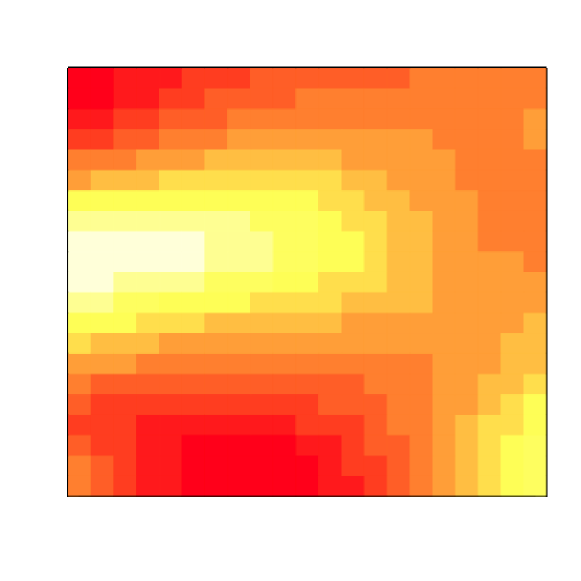
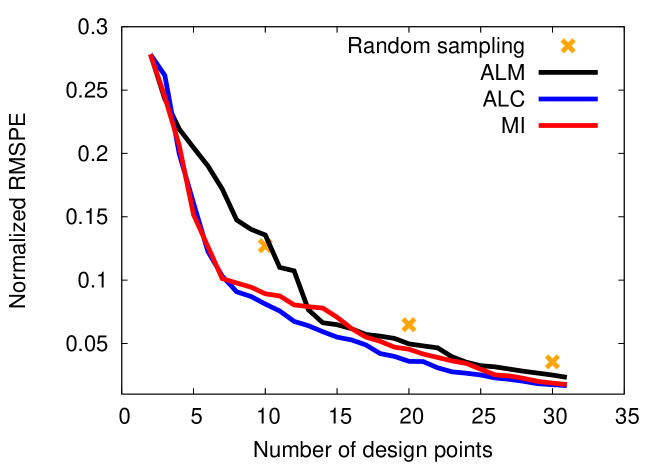
As a first example, we consider a realization of a stationary Gaussian random field with zero mean, and SE covariance function with σ2=1superscript𝜎21\sigma^{2}=1 and 𝝃=(0.8,0.5)T𝝃superscript0.80.5𝑇{\boldsymbol{\xi}}=\left(0.8,0.5\right)^{T}, on a 21×21212121\times 21 regular grid over [0,1]2superscript012[0,1]^{2}. The candidate set is a regular sub-grid of size 11×11111111\times 11. The remaining 320 design points are used to calculate the prediction accuracy. In all our numerical examples, the prediction accuracy is measured by the normalized RMSPE:

RMSPE=j=1m(y(𝒙j)y^(𝒙j))2m,RMSPEsubscriptsuperscript𝑚𝑗1superscript𝑦subscript𝒙𝑗^𝑦subscript𝒙𝑗2𝑚\operatorname{RMSPE}=\sqrt{\sum^{m}_{j=1}\dfrac{(y({\boldsymbol{x}}_{j})-\hat{y}({\boldsymbol{x}}_{j}))^{2}}{m}}, (25)

where the validation data set {𝒙j}j=1msubscriptsuperscriptsubscript𝒙𝑗𝑚𝑗1\{{\boldsymbol{x}}_{j}\}^{m}_{j=1} consists of m𝑚m input values at which the difference between the simulator output value y(𝒙j)𝑦subscript𝒙𝑗y({\boldsymbol{x}}_{j}) and the predicted value y^(𝒙j)^𝑦subscript𝒙𝑗\hat{y}({\boldsymbol{x}}_{j}) is evaluated. The normalized RMSPE is given by RMPSE/(maxjy(𝒙j)minjy(𝒙j))RMPSEsubscript𝑗𝑦subscript𝒙𝑗subscript𝑗𝑦subscript𝒙𝑗\operatorname{RMPSE}/(\max_{j}{y({\boldsymbol{x}}_{j})}-\min_{j}{y({\boldsymbol{x}}_{j})}).

Refer to caption
Refer to caption
Figure 1: Left: A realization of the stationary Gaussian random field. Right: Prediction errors.

Figure 1 shows results obtained for ALM, ALC and MI. The prediction errors are given as averages of ten tries with different initial two-point designs. The average performance of random sampling over 100 tries has also been included for comparison, and as expected, the sequential designs outperform random sampling. MI and ALC perform similarly. ALM performs the worst, partially because it systematically places most points on the boundary of the domain, and, as a result, not capturing well the large variation in the interior.

3.1.2 A practical issue with the MI criterion

Krause et al. [18] showed theoretically and demonstrated empirically that the MI criterion is a promising criterion for sequential design of sensor networks on a discrete space. In computer experiments, however, the design space is generally not discrete but a compact subset of psuperscript𝑝\mathbb{R}^{p} where p𝑝p can be quite large. For the MI criterion to be considered, we have to discretize 𝒳𝒳{\mathcal{X}} into a finite set 𝑿G𝒳subscript𝑿𝐺𝒳{\boldsymbol{X}}_{G}\subset{\mathcal{X}} of a grid G𝐺G. This is because for each candidate point 𝒙𝑿candsuperscript𝒙subscript𝑿𝑐𝑎𝑛𝑑{\boldsymbol{x}}^{*}\in{\boldsymbol{X}}_{cand}, we want to assign a GP emulator over the points of a finite set 𝑿G\(𝑿k𝒙)\subscript𝑿𝐺subscript𝑿𝑘superscript𝒙{\boldsymbol{X}}_{G}\backslash({\boldsymbol{X}}_{k}\cup{\boldsymbol{x}}^{*}) that approximates well 𝒳\(𝑿k𝒙)\𝒳subscript𝑿𝑘superscript𝒙{\mathcal{X}}\backslash({\boldsymbol{X}}_{k}\cup{\boldsymbol{x}}^{*}). Recall that 𝑿ksubscript𝑿𝑘{\boldsymbol{X}}_{k} is the set of design points at stage k𝑘k of the sequential design.

We have observed that the MI criterion (3.1) is very sensitive to the distribution of points in 𝑿Gsubscript𝑿𝐺{\boldsymbol{X}}_{G}. For example when the points of 𝑿Gsubscript𝑿𝐺{\boldsymbol{X}}_{G} are irregularly distributed, e.g., if some points are clustered, this criterion is unreliable. More specifically, if the criterion is evaluated at a point 𝒙𝑿candsuperscript𝒙subscript𝑿𝑐𝑎𝑛𝑑{\boldsymbol{x}}^{*}\in{\boldsymbol{X}}_{cand} that is close to a point in 𝑿G\(𝑿k𝒙)\subscript𝑿𝐺subscript𝑿𝑘superscript𝒙{\boldsymbol{X}}_{G}\backslash({\boldsymbol{X}}_{k}\cup{\boldsymbol{x}}^{*}), then the denominator s^G\(k𝒙)2(𝒙)subscriptsuperscript^𝑠2\𝐺𝑘superscript𝒙superscript𝒙\hat{s}^{2}_{G\backslash(k\cup{\boldsymbol{x}}^{*})}({\boldsymbol{x}}^{*}) can become very small, and, as a result, producing a high MI score. In this situation, the issue is that the location of 𝒙superscript𝒙{\boldsymbol{x}}^{*} in relation to the current design 𝑿ksubscript𝑿𝑘{\boldsymbol{X}}_{k}, which should be important factor, has little influence. This issue did not present itself in [18], since they considered an equidistant grid.

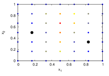
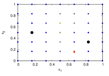
See Figure 2 for an illustrative example where the MI criterion performs poorly. Two cases are considered: an equidistant grid 𝑿Gsubscript𝑿𝐺{\boldsymbol{X}}_{G}, and 𝑿Gsubscript𝑿𝐺{\boldsymbol{X}}_{G} with an additional point (2/3,0.15)230.15(2/3,0.15), that is, 𝑿G{(2/3,0.15)}subscript𝑿𝐺230.15{\boldsymbol{X}}_{G}\cup\{(2/3,0.15)\}. A high MI score is marked in red, an intermediate score is yellow, and a low score is blue. The black dots are the points of design 𝑿ksubscript𝑿𝑘{\boldsymbol{X}}_{k}.

Refer to caption
Refer to caption
Figure 2: The score value of the MI criterion over a 7×7777\times 7 equidistant grid (Left), and of the same grid with an additional point at (2/3,0.15)230.15(2/3,0.15) (Right).

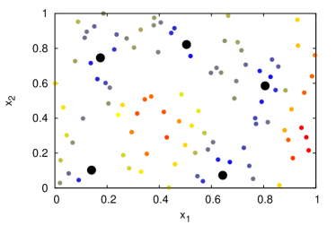
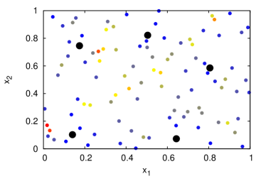
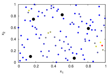
Two different choices of 𝑿Gsubscript𝑿𝐺{\boldsymbol{X}}_{G} can result in highly conflicting MI scores, as demonstrated in Figure 3 with two different maximin LHDs of size 100. Evidently, the MI criterion is not robust whenever the points are irregularly spaced. Moreover, for moderate to high dimensional spaces, typical of computer experiments, equidistant grids are too large to consider.
Refer to caption
Refer to caption
Figure 3: Given a design 𝑿5subscript𝑿5{\boldsymbol{X}}_{5}, the score value of the MI criterion is displayed for two maximin LHD candidate sets of size 100100100.

3.2 Mutual information for computer experiments

In this section we present a sequential design algorithm called MICE (Mutual Information for Computer Experiments) for prediction. The algorithm uses on a modified MI criterion, and the correlation parameters are estimated adaptively using maximum likelihood. We also suggest that discretization 𝑿Gsubscript𝑿𝐺{\boldsymbol{X}}_{G} of 𝒳𝒳{\mathcal{X}} should not be held fixed, but instead a new 𝑿Gsubscript𝑿𝐺{\boldsymbol{X}}_{G} should be sampled at each iteration.

3.2.1 The MICE criterion: a modified MI criterion

We modify the MI criterion by introducing a parameter τ2>0superscript𝜏20\tau^{2}>0 to the diagonal elements of the correlation matrix to smooth the prediction. Such a parameter is often called a nugget parameter. 𝑲𝝃subscript𝑲𝝃{\boldsymbol{K}}_{{\boldsymbol{\xi}}} is replaced by 𝑲𝝃,τ2=𝑲𝝃+τ2subscript𝑲𝝃superscript𝜏2subscript𝑲𝝃superscript𝜏2{\boldsymbol{K}}_{{\boldsymbol{\xi}},\tau^{2}}={\boldsymbol{K}}_{{\boldsymbol{\xi}}}+\tau^{2}\mathcal{I}, where \mathcal{I} is the n×n𝑛𝑛n\times n identity matrix. A nugget parameter τ2superscript𝜏2\tau^{2} is commonly used to stabilize the inversion, using the Cholesky decomposition, of a possibly ill-conditioned correlation matrix. When τ2superscript𝜏2\tau^{2} is introduced to achieve numerical stability, it is usually chosen to be very small. Moreover, Gramacy and Lee [13] argue in favor of using a nugget parameter to smooth the prediction. The BLUP model, Eq. (4), with a non-zero nugget is not a perfect interpolator of the data, and our Theorem 1 below clarifies the impact a nugget parameter has on the GP emulator variance for any point in 𝑿𝑿{\boldsymbol{X}}. Clearly, if τ2=0superscript𝜏20\tau^{2}=0, s^2(𝒙i)=0superscript^𝑠2subscript𝒙𝑖0\hat{s}^{2}({\boldsymbol{x}}_{i})=0 for 𝒙i𝑿subscript𝒙𝑖𝑿{\boldsymbol{x}}_{i}\in{\boldsymbol{X}}.

Theorem 1

For a GP emulator with constant mean on (𝐗,𝐲)𝐗𝐲({\boldsymbol{X}},{\boldsymbol{y}}), the predictive variance, Eq. (6), at any design point 𝐱i𝐗subscript𝐱𝑖𝐗{\boldsymbol{x}}_{i}\in{\boldsymbol{X}} can be written as

s^τ22(𝒙i)=σ2(τ2τ4eiT(𝑲+τ2)1ei+τ4(eiT(𝑲+τ2)11)21T(𝑲+τ2)11),subscriptsuperscript^𝑠2superscript𝜏2subscript𝒙𝑖superscript𝜎2superscript𝜏2superscript𝜏4superscriptsubscripte𝑖𝑇superscript𝑲superscript𝜏21subscripte𝑖superscript𝜏4superscriptsuperscriptsubscripte𝑖𝑇superscript𝑲superscript𝜏2112superscript1𝑇superscript𝑲superscript𝜏211\hat{s}^{2}_{\tau^{2}}({\boldsymbol{x}}_{i})=\sigma^{2}\left(\tau^{2}-\tau^{4}\textbf{e}_{i}^{T}({\boldsymbol{K}}+\tau^{2}\mathcal{I})^{-1}\textbf{e}_{i}+\tau^{4}\dfrac{(\textbf{e}_{i}^{T}({\boldsymbol{K}}+\tau^{2}\mathcal{I})^{-1}\textbf{1})^{2}}{\textbf{1}^{T}({\boldsymbol{K}}+\tau^{2}\mathcal{I})^{-1}\textbf{1}}\right), (26)

where τ2>0superscript𝜏20\tau^{2}>0 is a nugget parameter, and eisubscripte𝑖\textbf{e}_{i} is the i𝑖i-th unit vector.

According to Theorem 1, whenever τ2>0superscript𝜏20\tau^{2}>0 is added to the correlation matrix diagonal, the variance of a GP emulator at a design point consists of terms in the order of σ2τ2superscript𝜎2superscript𝜏2\sigma^{2}\tau^{2} and σ2τ4superscript𝜎2superscript𝜏4\sigma^{2}\tau^{4}. In practice, the nugget τ2superscript𝜏2\tau^{2} is usually orders of magnitude smaller than 1. In Eq. (26), the magnitude of the last term in the round brackets tends to be much smaller than the other two; hence, the predictive variance is here typically smaller than σ2τ2superscript𝜎2superscript𝜏2\sigma^{2}\tau^{2}. Moreover, as τ2superscript𝜏2\tau^{2} increases, the second and third term approaches τ2superscript𝜏2\tau^{2} and τ2/ksuperscript𝜏2𝑘\tau^{2}/k, respectively, where k𝑘k is the number of points in the design. This follows from that as τ2superscript𝜏2\tau^{2} increases the inverse matrix reduces to (𝑲+τ2)1τ2superscript𝑲superscript𝜏21superscript𝜏2({\boldsymbol{K}}+\tau^{2}\mathcal{I})^{-1}\approx\tau^{-2}\mathcal{I}. Hence, if τ2superscript𝜏2\tau^{2} is large enough, we can show by a simple calculation using Theorem 1 that s^τ22(𝒙i)σ2τ2/ksubscriptsuperscript^𝑠2superscript𝜏2subscript𝒙𝑖superscript𝜎2superscript𝜏2𝑘\hat{s}^{2}_{\tau^{2}}({\boldsymbol{x}}_{i})\approx\sigma^{2}\tau^{2}/k for 𝒙i𝑿ksubscript𝒙𝑖subscript𝑿𝑘{\boldsymbol{x}}_{i}\in{\boldsymbol{X}}_{k}.

In the sequential design, we define the MICE criterion as follows:

𝒙k+1=argmax𝒙𝑿cands^k2(𝒙)/s^G\(k𝒙)2(𝒙;τs2),subscript𝒙𝑘1subscriptargmax𝒙subscript𝑿𝑐𝑎𝑛𝑑subscriptsuperscript^𝑠2𝑘𝒙subscriptsuperscript^𝑠2\𝐺𝑘𝒙𝒙subscriptsuperscript𝜏2𝑠{\boldsymbol{x}}_{k+1}=\operatorname*{arg\ max}\limits_{{\boldsymbol{x}}\in{\boldsymbol{X}}_{cand}}\hat{s}^{2}_{k}({\boldsymbol{x}})/\hat{s}^{2}_{G\backslash(k\cup{\boldsymbol{x}})}({\boldsymbol{x}};\tau^{2}_{s}), (27)

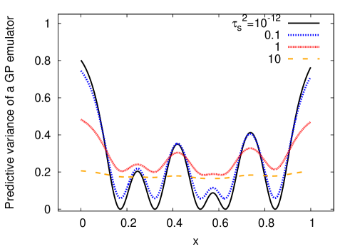
where a nugget parameter τs2>0superscriptsubscript𝜏𝑠20\tau_{s}^{2}>0 (s for smoothing) is added to the correlation matrix 𝑲𝑲{\boldsymbol{K}} of the GP on 𝑿G\(𝑿k𝒙)\subscript𝑿𝐺subscript𝑿𝑘𝒙{\boldsymbol{X}}_{G}\backslash({\boldsymbol{X}}_{k}\cup{\boldsymbol{x}}) (in the denominator) with the specific purpose of flattening its variance. The flattening of the variance is performed as a means of preventing the denominator term to be close to zero, which may happen whenever a candidate point 𝒙superscript𝒙{\boldsymbol{x}}^{*} is too close to a point in 𝑿G\(𝑿k𝒙)\subscript𝑿𝐺subscript𝑿𝑘superscript𝒙{\boldsymbol{X}}_{G}\backslash({\boldsymbol{X}}_{k}\cup{\boldsymbol{x}}^{*}). Figure 4 shows the predictive variance for different choices of τs2subscriptsuperscript𝜏2𝑠\tau^{2}_{s}.

Refer to caption
Figure 4: The predictive variance of a GP emulator as a function of τs2superscriptsubscript𝜏𝑠2\tau_{s}^{2} for a one-dimensional problem in domain [0,1]01[0,1].

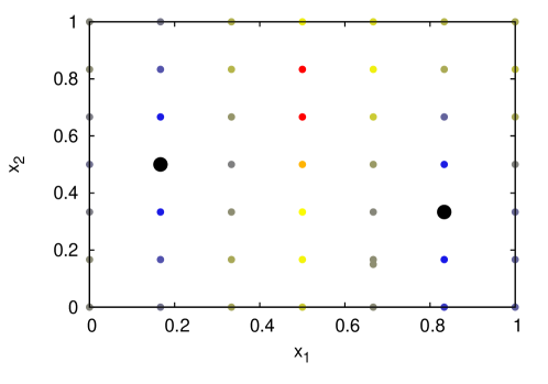
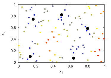
The sweet spot of τs2subscriptsuperscript𝜏2𝑠\tau^{2}_{s} is around 111, where the variance is not close to zero and the shape of the variance curve is well preserved. Hence our default choice is τs2=1subscriptsuperscript𝜏2𝑠1\tau^{2}_{s}=1. Figure 5 and 6 show MICE scores with τs2=1subscriptsuperscript𝜏2𝑠1\tau^{2}_{s}=1, which can be compared with the corresponding figures for MI (see Figure 2 and 3, respectively). By examining the figures, we can conclude that MICE is more robust than MI. For a simple regular grid, MICE and MI perform the same.
Refer to caption
Figure 5: The score values of the MICE criterion using τs2=1subscriptsuperscript𝜏2𝑠1\tau^{2}_{s}=1 for a 7×7777\times 7 equidistant grid with an additional candidate point at (2/3,0.15)230.15(2/3,0.15).
Refer to caption
Refer to caption
Figure 6: Given a design 𝑿5subscript𝑿5{\boldsymbol{X}}_{5}, the score values of the MICE criterion using τs2=1subscriptsuperscript𝜏2𝑠1\tau^{2}_{s}=1 are shown for two maximin LHD candidate sets of size 100100100.

3.2.2 Adaptivity

The original implementation of the MI algorithm assumed that the covariance is fully known, but that is rarely the case in modeling of computer experiments. Therefore, in our implementation, whenever the correlation parameters 𝝃𝝃{\boldsymbol{\xi}} are unknown, we provide point estimates that maximize the likelihood. This approach is described in Section 2.1. The MLEs of 𝝃𝝃{\boldsymbol{\xi}} are sequentially updated at each stage k𝑘k, denoted by 𝝃^ksubscript^𝝃𝑘\hat{{\boldsymbol{\xi}}}_{k}, by using all available input-output data. However, the updating may be skipped at some stages in order to make computational savings.
Refer to caption
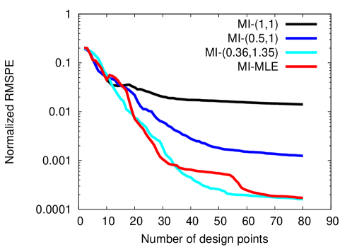
Figure 7: Prediction errors for the MI algorithm when using estimates of 𝝃𝝃{\boldsymbol{\xi}} (three guesses, and one using MLE updates).

The prediction errors for different choices of estimates for the correlation parameters are shown in Figure 7, where the example is the so-called Branin function, y(𝒙)=(x25.1x12/(4π2)+(5/π)x16)2+10(11/(8π))cos(x1)+10𝑦𝒙superscriptsubscript𝑥25.1superscriptsubscript𝑥124superscript𝜋25𝜋subscript𝑥16210118𝜋subscript𝑥110y({\boldsymbol{x}})=(x_{2}-5.1x_{1}^{2}/(4\pi^{2})+(5/\pi)x_{1}-6)^{2}+10(1-1/(8\pi))\cos(x_{1})+10, on a 21×21212121\times 21 regular grid over [5,10]×[0,15]2510015superscript2[-5,10]\times[0,15]\subset\mathbb{R}^{2}. A GP emulator is used with the Matérn correlation fixed at ν=5/2𝜈52\nu=5/2. Here, MI-MLE is the MI algorithm with the addition of a MLE step at each stage k𝑘k of the sequential design. For k<10𝑘10k<10, the tentative values (1,1)11(1,1) are assigned for 𝝃𝝃{\boldsymbol{\xi}}. Three fixed guesses of 𝝃𝝃{\boldsymbol{\xi}} are considered: (1,1)11(1,1), (0.5,1)0.51(0.5,1), and (0.36,1.35)0.361.35(0.36,1.35). The latter guess is the final MLEs obtained by MI-MLE. The results show the importance of having good estimates of the correlation parameters, and that the MLE method can greatly improve upon simple guesses.

3.2.3 The MICE algorithm

The MICE algorithm is outlined below with some details on some of the steps.

MICE algorithm:
Require: Function y(𝒙)𝑦𝒙y({\boldsymbol{x}}), GP emulator (𝒉()𝒉{\boldsymbol{h}}(\cdot),K(,;𝝃)𝐾𝝃K(\cdot,\cdot;{\boldsymbol{\xi}})), nugget parameters τ2superscript𝜏2\tau^{2} and τs2subscriptsuperscript𝜏2𝑠\tau^{2}_{s}, design space 𝒳𝒳{\mathcal{X}}, initial data (𝑿k,𝒚k)subscript𝑿𝑘subscript𝒚𝑘({\boldsymbol{X}}_{k},{\boldsymbol{y}}_{k}), discrete set size NGsubscript𝑁𝐺N_{G}, candidate set size Ncandsubscript𝑁𝑐𝑎𝑛𝑑N_{cand}, desired design size N𝑁N Step 1. MLE to obtain estimates 𝝃^ksubscript^𝝃𝑘\hat{{\boldsymbol{\xi}}}_{k} of 𝝃𝝃{\boldsymbol{\xi}} in K(,;𝝃^k)𝐾subscript^𝝃𝑘K(\cdot,\cdot;\hat{{\boldsymbol{\xi}}}_{k}) Step 2. Fit GP emulator to data (𝑿k,𝒚k)subscript𝑿𝑘subscript𝒚𝑘({\boldsymbol{X}}_{k},{\boldsymbol{y}}_{k}) Step 3. Generate a discrete set 𝑿Gsubscript𝑿𝐺{\boldsymbol{X}}_{G} of size NGsubscript𝑁𝐺N_{G}, and choose a candidate set 𝑿cand𝑿Gsubscript𝑿𝑐𝑎𝑛𝑑subscript𝑿𝐺{\boldsymbol{X}}_{cand}\subseteq{\boldsymbol{X}}_{G} Step 4. Solve 𝒙k+1=argmax𝒙𝑿cands^k2(𝒙;𝝃^k,τ2)/s^G\(k𝒙)2(𝒙;𝝃^k,max{τ2,τs2})subscript𝒙𝑘1subscriptargmax𝒙subscript𝑿𝑐𝑎𝑛𝑑subscriptsuperscript^𝑠2𝑘𝒙subscript^𝝃𝑘superscript𝜏2subscriptsuperscript^𝑠2\𝐺𝑘𝒙𝒙subscript^𝝃𝑘superscript𝜏2superscriptsubscript𝜏𝑠2{\boldsymbol{x}}_{k+1}=\operatorname*{arg\ max}\limits_{{\boldsymbol{x}}\in{\boldsymbol{X}}_{cand}}\hat{s}^{2}_{k}({\boldsymbol{x}};\hat{{\boldsymbol{\xi}}}_{k},\tau^{2})/\hat{s}^{2}_{G\backslash(k\cup{\boldsymbol{x}})}({\boldsymbol{x}};\hat{{\boldsymbol{\xi}}}_{k},\max\{\tau^{2},\tau_{s}^{2}\}) Step 5. Evaluate yk+1=y(𝒙k+1)subscript𝑦𝑘1𝑦subscript𝒙𝑘1y_{k+1}=y({\boldsymbol{x}}_{k+1}), and let 𝑿k+1=𝑿k𝒙k+1subscript𝑿𝑘1subscript𝑿𝑘subscript𝒙𝑘1{\boldsymbol{X}}_{k+1}={\boldsymbol{X}}_{k}\cup{\boldsymbol{x}}_{k+1} and 𝒚k+1=𝒚kyk+1subscript𝒚𝑘1subscript𝒚𝑘subscript𝑦𝑘1{\boldsymbol{y}}_{k+1}={\boldsymbol{y}}_{k}\cup y_{k+1} Step 6. If k+1=N𝑘1𝑁k+1=N, then stop; otherwise let k=k+1𝑘𝑘1k=k+1, and go to step 1 Output: DN=(𝑿ND_{N}=({\boldsymbol{X}}_{N},𝒚N){\boldsymbol{y}}_{N}) of size N𝑁N
In step 3, we suggest that 𝑿Gsubscript𝑿𝐺{\boldsymbol{X}}_{G} is sampled in the design space 𝒳𝒳{\mathcal{X}}, instead of keeping 𝑿Gsubscript𝑿𝐺{\boldsymbol{X}}_{G} fixed throughout. In our examples, the size of 𝑿Gsubscript𝑿𝐺{\boldsymbol{X}}_{G} is k+NG𝑘subscript𝑁𝐺k+N_{G}, where k𝑘k is the number of points of Xksubscript𝑋𝑘X_{k}. The additional NGsubscript𝑁𝐺N_{G} points are generated picking a LHD from a set of LHDs by maximizing the minimum distance between the points in this LHD and the current design 𝑿ksubscript𝑿𝑘{\boldsymbol{X}}_{k}. In step 4, the MICE criterion is evaluated for all 𝒙𝑿cand𝒙subscript𝑿𝑐𝑎𝑛𝑑{\boldsymbol{x}}\in{\boldsymbol{X}}_{cand}. The choice of τs2subscriptsuperscript𝜏2𝑠\tau^{2}_{s} is critical; more on this in Section 5. Note that the parameter τs2subscriptsuperscript𝜏2𝑠\tau^{2}_{s} is introduced to the GP for design 𝑿G\(𝑿k𝒙)\subscript𝑿𝐺subscript𝑿𝑘𝒙{\boldsymbol{X}}_{G}\backslash({\boldsymbol{X}}_{k}\cup{\boldsymbol{x}}), and not to the GP for design 𝑿ksubscript𝑿𝑘{\boldsymbol{X}}_{k}. Although, a nugget parameter τ2>0superscript𝜏20\tau^{2}>0 can still be introduced to any GP for other purposes such as achieving numerical stability (typically much smaller than τs2=1subscriptsuperscript𝜏2𝑠1\tau^{2}_{s}=1). We assume that the correlation parameters are the same for the GP on 𝑿G(𝑿k𝒙)subscript𝑿𝐺subscript𝑿𝑘𝒙{\boldsymbol{X}}_{G}\cup({\boldsymbol{X}}_{k}\cup{\boldsymbol{x}}) as for the GP on 𝑿ksubscript𝑿𝑘{\boldsymbol{X}}_{k}.

3.2.4 Near optimality results

We here provide an approximative bound of optimality for the MICE algorithm based on near optimality results in [18] for the MI algorithm under known 𝝃𝝃{\boldsymbol{\xi}}. More generally, our results account for the possibility that a different nugget parameter is used for the GP over 𝑿ksubscript𝑿𝑘{\boldsymbol{X}}_{k} than the over 𝑿𝑮\𝑿k𝒙\subscript𝑿𝑮subscript𝑿𝑘𝒙{\boldsymbol{X}}_{\boldsymbol{G}}\backslash{\boldsymbol{X}}_{k}\cup{\boldsymbol{x}}.

Theorem 2

Let Y(𝐱)𝑌𝐱Y({\boldsymbol{x}}) be a second-order stationary Gaussian process with constant mean on a compact set 𝒳p𝒳superscript𝑝{\mathcal{X}}\subset\mathbb{R}^{p} with a continuous correlation function K(𝐱,𝐱):𝒳×𝒳0+:𝐾𝐱superscript𝐱𝒳𝒳superscriptsubscript0K({\boldsymbol{x}},{\boldsymbol{x}}^{\prime}):{\mathcal{X}}\times{\mathcal{X}}\to\mathbb{R}_{0}^{+}. Assume that we have estimates 𝛏^ksubscript^𝛏𝑘\hat{{\boldsymbol{\xi}}}_{k} for 𝛏𝛏{\boldsymbol{\xi}} at stage k𝑘k that satisfy for some constant α>0𝛼0\alpha>0, |K(𝐱,𝐱;𝛏)K(𝐱,𝐱;𝛏^k)|α𝐾𝐱superscript𝐱𝛏𝐾𝐱superscript𝐱subscript^𝛏𝑘𝛼|K({\boldsymbol{x}},{\boldsymbol{x}}^{\prime};{\boldsymbol{\xi}})-K({\boldsymbol{x}},{\boldsymbol{x}}^{\prime};\hat{{\boldsymbol{\xi}}}_{k})|\leq\alpha. Then, for any ε>0𝜀0\varepsilon>0, and any finite number N𝑁N, there exists a discretization 𝐗Gsubscript𝐗𝐺{\boldsymbol{X}}_{G} of mesh width δ>0𝛿0\delta>0 such that MICE is guaranteed to select a design DN=(𝐗N,𝐲N)subscript𝐷𝑁subscript𝐗𝑁subscript𝐲𝑁D_{N}=({\boldsymbol{X}}_{N},{\boldsymbol{y}}_{N}) with N𝑁N design points, where N2|𝐆|𝑁2𝐆N\leq 2|{\boldsymbol{G}}|, for which

MI(DN)(11/e)(OPTNε2(ασ1τ1)2N4(1+N3/2)2N3N|τs2τ2|/τs2),𝑀𝐼subscript𝐷𝑁11𝑒𝑂𝑃𝑇𝑁𝜀2superscript𝛼superscript𝜎1superscript𝜏12superscript𝑁4superscript1superscript𝑁322superscript𝑁3𝑁superscriptsubscript𝜏𝑠2superscript𝜏2subscriptsuperscript𝜏2𝑠MI(D_{N})\geq(1-1/e)(OPT-N\varepsilon-2(\alpha\sigma^{-1}\tau^{-1})^{2}N^{4}(1+N^{3/2})^{2}-N^{3}\sqrt{N}|\tau_{s}^{2}-\tau^{2}|/\tau^{2}_{s}),

where e𝑒e is the base of the natural logarithm, OPT𝑂𝑃𝑇OPT is the value of the mutual information for the optimal design of size N𝑁N, and, τ2superscript𝜏2\tau^{2} and τs2subscriptsuperscript𝜏2𝑠\tau^{2}_{s} are nugget parameters in the correlation matrices for 𝐗ksubscript𝐗𝑘{\boldsymbol{X}}_{k}, and 𝐗G\𝐗k\subscript𝐗𝐺subscript𝐗𝑘{\boldsymbol{X}}_{G}\backslash{\boldsymbol{X}}_{k}, respectively.

Under perfect conditions the upper bound in Theorem 2 guarantees a performance within 63%percent\% of the optimum. The term Nε>0𝑁𝜀0N\varepsilon>0 is essentially zero as long as the discretization 𝑿Gsubscript𝑿𝐺{\boldsymbol{X}}_{G} is fine enough. The term 2(ασ1τ1)2N4(1+N3/2)22superscript𝛼superscript𝜎1superscript𝜏12superscript𝑁4superscript1superscript𝑁3222(\alpha\sigma^{-1}\tau^{-1})^{2}N^{4}(1+N^{3/2})^{2} is non-zero in the presence of parameter uncertainty, and the term N3N|τs2τ2|/τs2superscript𝑁3𝑁superscriptsubscript𝜏𝑠2superscript𝜏2subscriptsuperscript𝜏2𝑠N^{3}\sqrt{N}|\tau_{s}^{2}-\tau^{2}|/\tau^{2}_{s} appears when a nugget τ2superscript𝜏2\tau^{2} is used for the GP emulator over 𝑿ksubscript𝑿𝑘{\boldsymbol{X}}_{k}. Our extension of the approximative bound of optimality to MICE reveals the effect of τs2subscriptsuperscript𝜏2𝑠\tau^{2}_{s} on the performance. Our default choice τs2=1subscriptsuperscript𝜏2𝑠1\tau^{2}_{s}=1 is not causing the algorithm to diverge too much from MI, as long as τ2superscript𝜏2\tau^{2} is not much larger than τs2subscriptsuperscript𝜏2𝑠\tau^{2}_{s}. In addition, whenever the correlation parameters are poorly estimated, the optimality bound is not sharp. To increase our understanding of the MICE behavior with respect to the choice of 𝑿Gsubscript𝑿𝐺{\boldsymbol{X}}_{G}, we provide the following theorem:

Theorem 3

Let Y(𝐱)𝑌𝐱Y({\boldsymbol{x}}) be a second-order stationary Gaussian process with constant mean on a compact subset 𝒳𝒳{\mathcal{X}} of psuperscript𝑝\mathbb{R}^{p} with a Lipschitz-continuous correlation function. Then, for any ε>0𝜀0\varepsilon>0, there exists a regular grid 𝐗G𝒳subscript𝐗𝐺𝒳{\boldsymbol{X}}_{G}\subset{\mathcal{X}} with grid spacing δ=2ε/(pKL)𝛿2𝜀𝑝subscript𝐾𝐿\delta=2\varepsilon/(\sqrt{p}K_{L}) so that for any untried point 𝐱𝒳superscript𝐱𝒳{\boldsymbol{x}}^{*}\in{\mathcal{X}} the predictive variance s^τ22(𝐱)subscriptsuperscript^𝑠2superscript𝜏2𝐱\hat{s}^{2}_{\tau^{2}}({\boldsymbol{x}}) is bounded as

τ4b1(τ2)ε<σ2s^τ22(𝒙)τ2<τ4b2(τ2)+ε,superscript𝜏4subscript𝑏1superscript𝜏2𝜀superscript𝜎2subscriptsuperscript^𝑠2superscript𝜏2superscript𝒙superscript𝜏2superscript𝜏4subscript𝑏2superscript𝜏2𝜀-\tau^{4}b_{1}(\tau^{2})-\varepsilon<\sigma^{-2}\hat{s}^{2}_{\tau^{2}}({\boldsymbol{x}}^{*})-\tau^{2}<\tau^{4}b_{2}(\tau^{2})+\varepsilon,

where

b1(τ2)=max{eiT(𝑲+τ2)1ei:𝒙i𝑿G},subscript𝑏1superscript𝜏2:superscriptsubscripte𝑖𝑇superscript𝑲superscript𝜏21subscripte𝑖subscript𝒙𝑖subscript𝑿𝐺b_{1}(\tau^{2})=\max\left\{\textbf{e}_{i}^{T}({\boldsymbol{K}}+\tau^{2}\mathcal{I})^{-1}\textbf{e}_{i}:{\boldsymbol{x}}_{i}\in{\boldsymbol{X}}_{G}\right\},

and

b2(τ2)=max{(eiT(𝑲+τ2)11)21T(𝑲+τ2)11:𝒙i𝑿G},subscript𝑏2superscript𝜏2:superscriptsuperscriptsubscripte𝑖𝑇superscript𝑲superscript𝜏2112superscript1𝑇superscript𝑲superscript𝜏211subscript𝒙𝑖subscript𝑿𝐺b_{2}(\tau^{2})=\max\left\{\dfrac{(\textbf{e}_{i}^{T}({\boldsymbol{K}}+\tau^{2}\mathcal{I})^{-1}\textbf{1})^{2}}{\textbf{1}^{T}({\boldsymbol{K}}+\tau^{2}\mathcal{I})^{-1}\textbf{1}}:{\boldsymbol{x}}_{i}\in{\boldsymbol{X}}_{G}\right\},

where \mathcal{I} is the identity matrix, and ensubscripte𝑛\textbf{e}_{n} the i𝑖i-th unit vector for member 𝐱isubscript𝐱𝑖{\boldsymbol{x}}_{i} of 𝐗Gsubscript𝐗𝐺{\boldsymbol{X}}_{G}. Here KLsubscript𝐾𝐿K_{L} is the Lipschitz constant for s^τ22(𝐱)subscriptsuperscript^𝑠2superscript𝜏2𝐱\hat{s}^{2}_{\tau^{2}}({\boldsymbol{x}}) over 𝒳𝒳{\mathcal{X}}.

Theorem 3 tells us that when 𝑿Gsubscript𝑿𝐺{\boldsymbol{X}}_{G} is a regular grid dense enough in 𝒳𝒳{\mathcal{X}}, while τ2superscript𝜏2\tau^{2} and τs2superscriptsubscript𝜏𝑠2\tau_{s}^{2} are small enough, MICE is equivalent to ALM. In fact, MICE also behaves as ALM if 𝑿Gsubscript𝑿𝐺{\boldsymbol{X}}_{G} more dense, and τs2superscriptsubscript𝜏𝑠2\tau_{s}^{2} large enough so that (𝑲+τ2)1=τ2superscript𝑲superscript𝜏21superscript𝜏2({\boldsymbol{K}}+\tau^{2}\mathcal{I})^{-1}=\tau^{-2}\mathcal{I} (approximately), since according to Theorem 3, as ε>0𝜀0\varepsilon>0 becomes arbitrary small, then 0<s^G\(k𝒙)2(𝒙)<ε0subscriptsuperscript^𝑠2\𝐺𝑘𝒙𝒙𝜀0<\hat{s}^{2}_{G\backslash(k\cup{\boldsymbol{x}})}({\boldsymbol{x}})<\varepsilon. This can be seen in Figure 4. Nonetheless, with τs2=1superscriptsubscript𝜏𝑠21\tau_{s}^{2}=1, MICE is not expected to behave as ALM. Similarly, MI behaves as ALM whenever 𝑿Gsubscript𝑿𝐺{\boldsymbol{X}}_{G} is dense in 𝒳𝒳{\mathcal{X}}, and τ2superscript𝜏2\tau^{2} is very small. The prerequisites of Theorem 3 hold in our numerical tests, because both the SE correlation function and Matérn correlation with ν=5/2𝜈52\nu=5/2 are continuously differentiable (hence Lipschitz continuous) [14].

3.2.5 A computational improvement

In MICE, we compute s^G\(k𝒙)2(𝒙)superscriptsubscript^𝑠\𝐺𝑘𝒙2𝒙\hat{s}_{G\backslash(k\cup{\boldsymbol{x}})}^{2}({\boldsymbol{x}}) for all 𝒙𝑿cand𝒙subscript𝑿𝑐𝑎𝑛𝑑{\boldsymbol{x}}\in{\boldsymbol{X}}_{cand}, which requires the Cholesky decomposition of a (NGk1)×(NGk1)subscript𝑁𝐺𝑘1subscript𝑁𝐺𝑘1(N_{G}-k-1)\times(N_{G}-k-1) correlation matrix 𝑲G\(k𝒙)subscript𝑲\𝐺𝑘𝒙{\boldsymbol{K}}_{G\backslash(k\cup{\boldsymbol{x}})}, where NGsubscript𝑁𝐺N_{G} is the number of points in 𝑿Gsubscript𝑿𝐺{\boldsymbol{X}}_{G}. This is a computationally intensive task if NGsubscript𝑁𝐺N_{G} is large. To overcome this, we use the following implementation which only requires a single Cholesky decomposition. First, invert the correlation matrix 𝑲G\ksubscript𝑲\𝐺𝑘{\boldsymbol{K}}_{G\backslash k}. Then, exploit the partitioned inverse formula for matrices in block-form. That is, the inverse of

𝑲G\k=(𝑲𝒌(𝒙)𝒌T(𝒙)TK(𝒙,𝒙))subscript𝑲\𝐺𝑘subscript𝑲superscript𝒌𝒙subscriptsuperscript𝒌𝑇superscript𝒙𝑇𝐾𝒙𝒙{\boldsymbol{K}}_{G\backslash k}=\left(\begin{array}[]{cc}{\boldsymbol{K}}_{*}&{\boldsymbol{k}}^{*}({\boldsymbol{x}})\\ {\boldsymbol{k}}^{T}_{*}({\boldsymbol{x}})^{T}&K({\boldsymbol{x}},{\boldsymbol{x}})\end{array}\right) (28)

can be written as:

𝑲G\k1=(𝑩𝒃12𝒃21b)superscriptsubscript𝑲\𝐺𝑘1𝑩subscript𝒃12subscript𝒃21𝑏{\boldsymbol{K}}_{G\backslash k}^{-1}=\left(\begin{array}[]{cc}{\boldsymbol{B}}&{\boldsymbol{b}}_{12}\\ {\boldsymbol{b}}_{21}&b\end{array}\right) (29)

where 𝑲=𝑲G\(k𝒙)subscript𝑲subscript𝑲\𝐺𝑘𝒙{\boldsymbol{K}}_{*}={\boldsymbol{K}}_{G\backslash(k\cup{\boldsymbol{x}})}, and 𝒌(𝒙)=𝒌G\(k𝒙)(𝒙)subscript𝒌𝒙subscript𝒌\𝐺𝑘𝒙𝒙{\boldsymbol{k}}_{*}({\boldsymbol{x}})={\boldsymbol{k}}_{G\backslash(k\cup{\boldsymbol{x}})}({\boldsymbol{x}}). Here 𝑩=𝑲1+1k𝑲1𝒌(𝒙)𝒌T(𝒙)𝑲1𝑩superscriptsubscript𝑲11𝑘superscriptsubscript𝑲1subscript𝒌𝒙superscriptsubscript𝒌𝑇𝒙superscriptsubscript𝑲1{\boldsymbol{B}}={\boldsymbol{K}}_{*}^{-1}+\frac{1}{k}{\boldsymbol{K}}_{*}^{-1}{\boldsymbol{k}}_{*}({\boldsymbol{x}}){\boldsymbol{k}}_{*}^{T}({\boldsymbol{x}}){\boldsymbol{K}}_{*}^{-1}, 𝒃12=1k𝑲1𝒌(𝒙)subscript𝒃121𝑘superscriptsubscript𝑲1subscript𝒌𝒙{\boldsymbol{b}}_{12}=-\frac{1}{k}{\boldsymbol{K}}_{*}^{-1}{\boldsymbol{k}}_{*}({\boldsymbol{x}}), 𝒃21=1k𝒌T(𝒙)𝑲1subscript𝒃211𝑘superscriptsubscript𝒌𝑇𝒙superscriptsubscript𝑲1{\boldsymbol{b}}_{21}=-\frac{1}{k}{\boldsymbol{k}}_{*}^{T}({\boldsymbol{x}}){\boldsymbol{K}}_{*}^{-1}, and b=1/(K(𝒙,𝒙)𝒌T(𝒙)T𝑲1𝒌(𝒙))𝑏1𝐾𝒙𝒙superscriptsubscript𝒌𝑇superscript𝒙𝑇superscriptsubscript𝑲1subscript𝒌𝒙b=1/(K({\boldsymbol{x}},{\boldsymbol{x}})-{\boldsymbol{k}}_{*}^{T}({\boldsymbol{x}})^{T}{\boldsymbol{K}}_{*}^{-1}{\boldsymbol{k}}_{*}({\boldsymbol{x}})). This relates 𝑲G\(k𝒙)1superscriptsubscript𝑲\𝐺𝑘𝒙1{\boldsymbol{K}}_{G\backslash(k\cup{\boldsymbol{x}})}^{-1} to 𝑲G\k1superscriptsubscript𝑲\𝐺𝑘1{\boldsymbol{K}}_{G\backslash k}^{-1} for any 𝒙𝑿G\k𝒙subscript𝑿\𝐺𝑘{\boldsymbol{x}}\in{\boldsymbol{X}}_{G\backslash k} as follows: given 𝑲G\k1superscriptsubscript𝑲\𝐺𝑘1{\boldsymbol{K}}_{G\backslash k}^{-1}, we can obtain 𝑩𝑩{\boldsymbol{B}}, 𝒃12subscript𝒃12{\boldsymbol{b}}_{12}, 𝒃21subscript𝒃21{\boldsymbol{b}}_{21} and b𝑏b, directly from Eq. (29), and then we find that 𝑲G\(k𝒙)1=𝑩1b𝒃12𝒃21superscriptsubscript𝑲\𝐺𝑘𝒙1𝑩1𝑏subscript𝒃12subscript𝒃21{\boldsymbol{K}}_{G\backslash(k\cup{\boldsymbol{x}})}^{-1}={\boldsymbol{B}}-\frac{1}{b}{\boldsymbol{b}}_{12}{\boldsymbol{b}}_{21}. Therefore, 𝑲G\(k𝒙)1superscriptsubscript𝑲\𝐺𝑘𝒙1{\boldsymbol{K}}_{G\backslash(k\cup{\boldsymbol{x}})}^{-1} can be obtained from 𝑲G\k1superscriptsubscript𝑲\𝐺𝑘1{\boldsymbol{K}}_{G\backslash k}^{-1} in 𝒪((NGk)2)𝒪superscriptsubscript𝑁𝐺𝑘2\mathcal{O}((N_{G}-k)^{2}).

3.2.6 Example: a visualization of the design selection

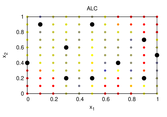
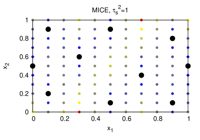
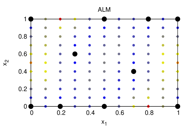
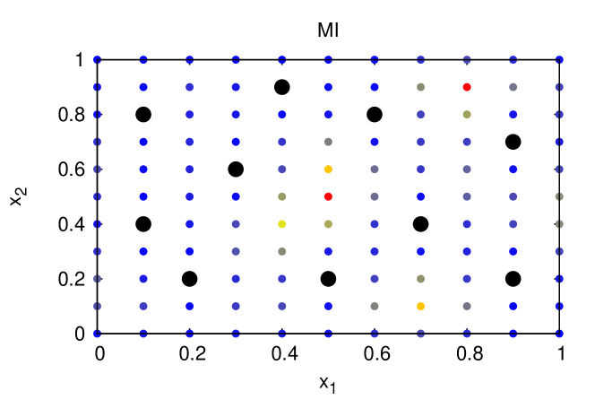
Design selection with ALM, ALC, MI, and MICE, on [0,1]2superscript012[0,1]^{2} are shown in Figure 8. A GP emulator with a constant mean is used with a fixed Matérn covariance using σ2=1superscript𝜎21\sigma^{2}=1, ν=5/2𝜈52\nu=5/2 and 𝝃=(0.4,1)𝝃0.41{\boldsymbol{\xi}}=(0.4,1). The black-solid dots are design points, and the others are candidate points with the color representing the score value (red-high, blue-low) for the different design criteria. The initial design consists of the points (0.3,0.6)0.30.6(0.3,0.6) and (0.7,0.4)0.70.4(0.7,0.4). MICE with τs2=1subscriptsuperscript𝜏2𝑠1\tau^{2}_{s}=1 and ALC produce centered and well-spaced designs, whereas ALM focuses on the boundary. MI is the criterion most reluctant to select boundary points.
Refer to captionRefer to caption
Figure 8: Design selection with ALM, ALC, MI and MICE on [0,1]2superscript012[0,1]^{2}

4 Computational complexity

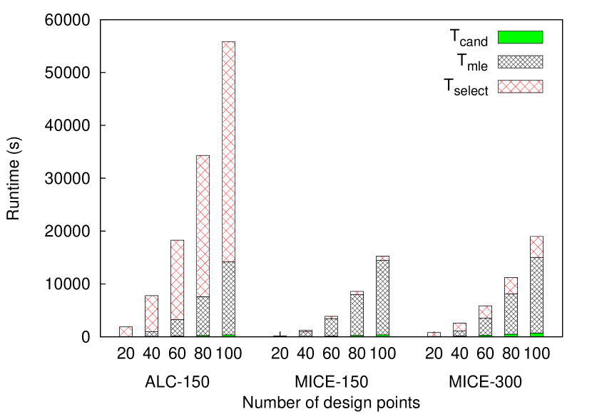
For the sequential algorithms the total computational cost to obtain a design 𝑿Nsubscript𝑿𝑁{\boldsymbol{X}}_{N} of size N𝑁N may be divided into the cost to fit the GP emulator (in our case using MLE), the cost to generate the candidate set 𝑿candsubscript𝑿𝑐𝑎𝑛𝑑{\boldsymbol{X}}_{cand}, and the cost to evaluate a design criterion over the candidate points:

Ttotal=Tmle+Tcand+Tselect.subscript𝑇𝑡𝑜𝑡𝑎𝑙subscript𝑇𝑚𝑙𝑒subscript𝑇𝑐𝑎𝑛𝑑subscript𝑇𝑠𝑒𝑙𝑒𝑐𝑡T_{total}=T_{mle}+T_{cand}+T_{select}. (30)

The time complexity to compute the MLEs is in 𝒪𝒪\mathcal{O}(pN2+NmleNω𝑝superscript𝑁2subscript𝑁𝑚𝑙𝑒superscript𝑁𝜔pN^{2}+N_{mle}N^{\omega}), where ω>0𝜔0\omega>0 is related to the efficiency of the algorithm for matrix inversion: for naïve Gaussian elimination ω=3𝜔3\omega=3, and for Strassen’s algorithm ω=log2(7)𝜔subscript27\omega=\log_{2}{\left(7\right)}. The term pN2𝑝superscript𝑁2pN^{2} is the number of operations needed to determine the distances between distinct pairs of points in 𝑿𝑿{\boldsymbol{X}} (which is N(N1)/2𝑁𝑁12N(N-1)/2). The second term, NmleNωsubscript𝑁𝑚𝑙𝑒superscript𝑁𝜔N_{mle}N^{\omega}, is the time complexity of MLE, which is directly related to the cost of inverting the correlation matrix 𝑲𝝃subscript𝑲𝝃{\boldsymbol{K}}_{{\boldsymbol{\xi}}}, Nmlesubscript𝑁𝑚𝑙𝑒N_{mle} times. Nmlesubscript𝑁𝑚𝑙𝑒N_{mle} is the number of trial points visited during the optimization to find the MLEs of 𝝃𝝃{\boldsymbol{\xi}}. To train the GP emulator, that is to say, determine the weights 𝝀𝝀{\boldsymbol{\lambda}} of the corresponding BLUP model (4), only matrix multiplications (each of order 𝒪(N2)𝒪superscript𝑁2\mathcal{O}\left(N^{2}\right)) are required. The time to evaluate the mean of the GP emulator at an untried point is 𝒪(pN)𝒪𝑝𝑁\mathcal{O}\left(pN\right), and to evaluate the variance is 𝒪(pN2)𝒪𝑝superscript𝑁2\mathcal{O}\left(pN^{2}\right).

Table 1: Time complexity for ALM, ALC and MICE.
Algorithm Total time complexity for design size N𝑁N
ALM 𝒪(NmleN1+ω+NcandpN2)𝒪subscript𝑁𝑚𝑙𝑒superscript𝑁1𝜔subscript𝑁𝑐𝑎𝑛𝑑𝑝superscript𝑁2\mathcal{O}\left(N_{mle}N^{1+\omega}+N_{cand}pN^{2}\right)
ALC 𝒪(NmleN1+ω+NcandNrefpN3)𝒪subscript𝑁𝑚𝑙𝑒superscript𝑁1𝜔subscript𝑁𝑐𝑎𝑛𝑑subscript𝑁𝑟𝑒𝑓𝑝superscript𝑁3\mathcal{O}\left(N_{mle}N^{1+\omega}+N_{cand}N_{ref}pN^{3}\right)
MICE 𝒪(NmleN1+ω+N(NGN)ω+NcandpN3+NcandNp(NGN)2)𝒪subscript𝑁𝑚𝑙𝑒superscript𝑁1𝜔𝑁superscriptsubscript𝑁𝐺𝑁𝜔subscript𝑁𝑐𝑎𝑛𝑑𝑝superscript𝑁3subscript𝑁𝑐𝑎𝑛𝑑𝑁𝑝superscriptsubscript𝑁𝐺𝑁2\mathcal{O}\left(N_{mle}N^{1+\omega}+N(N_{G}-N)^{\omega}+N_{cand}pN^{3}+N_{cand}Np(N_{G}-N)^{2}\right)

The computational complexity for the different algorithms is presented in Table 1. For ALC, we have adopted formulation (18), which is the formulation with lowest computational cost. The time complexity for a single ALM step is 𝒪(pk2+Nmlekω+Ncandpk)𝒪𝑝superscript𝑘2subscript𝑁𝑚𝑙𝑒superscript𝑘𝜔subscript𝑁𝑐𝑎𝑛𝑑𝑝𝑘\mathcal{O}\left(pk^{2}+N_{mle}k^{\omega}+N_{cand}pk\right), where k𝑘k is the current design size. The total cost for ALM is 𝒪(pN3+NmleN1+ω+NcandpN2)𝒪𝑝superscript𝑁3subscript𝑁𝑚𝑙𝑒superscript𝑁1𝜔subscript𝑁𝑐𝑎𝑛𝑑𝑝superscript𝑁2\mathcal{O}\left(pN^{3}+N_{mle}N^{1+\omega}+N_{cand}pN^{2}\right), where N𝑁N is the final design size. Nrefsubscript𝑁𝑟𝑒𝑓N_{ref} is specific to ALC, and is the number of reference points used for averaging over the design space.

Usually, NrefNcandNproportional-tosubscript𝑁𝑟𝑒𝑓subscript𝑁𝑐𝑎𝑛𝑑proportional-to𝑁N_{ref}\propto N_{cand}\propto N, NGNproportional-tosubscript𝑁𝐺𝑁N_{G}\propto N, and ω=3𝜔3\omega=3. The expressions in Table 1 can thus be written as 𝒪(NmleN4+pN3)𝒪subscript𝑁𝑚𝑙𝑒superscript𝑁4𝑝superscript𝑁3\mathcal{O}\left(N_{mle}N^{4}+pN^{3}\right) for ALM; 𝒪(NmleN4+pN5)𝒪subscript𝑁𝑚𝑙𝑒superscript𝑁4𝑝superscript𝑁5\mathcal{O}\left(N_{mle}N^{4}+pN^{5}\right) for ALC, and 𝒪(NmleN4+pN4)𝒪subscript𝑁𝑚𝑙𝑒superscript𝑁4𝑝superscript𝑁4\mathcal{O}\left(N_{mle}N^{4}+pN^{4}\right) for MICE. Observe that ALM has a much lower computational complexity than the others, and ALC is computationally prohibitive for large N𝑁N. MICE is computationally cheaper than ALC, as long as the ratio (NGN)/Nsubscript𝑁𝐺𝑁𝑁(N_{G}-N)/N is not too large. In the computer experiment setting, NGsubscript𝑁𝐺N_{G} can be chosen to not be too large out of computational convenience.

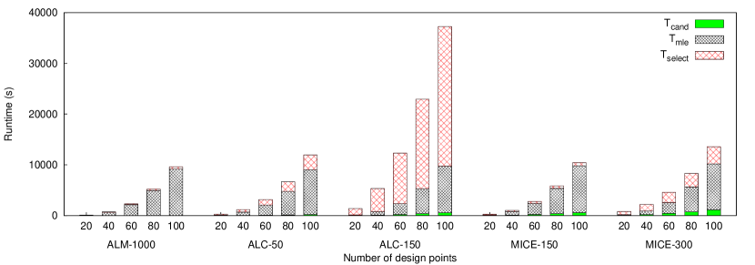
Because the maximum likelihood often is the most expensive step, NmleN1+ωsubscript𝑁𝑚𝑙𝑒superscript𝑁1𝜔N_{mle}N^{1+\omega}, a reduction in cost can be achieved by only updating the MLEs of 𝝃𝝃{\boldsymbol{\xi}} at every i𝑖i-th step, for some number i𝑖i. This tends to reduce Tmlesubscript𝑇𝑚𝑙𝑒T_{mle} substantially, giving MICE a significant advantage over ALC.
Refer to caption
Figure 9: Running time of the different sequential design algorithms for selecting designs of different fixed sizes. The study is on the Oscillatory function over [0,1]4superscript014[0,1]^{4}.

The cost to generate candidate sets varies depending on the choice of sampling technique and the desired size. For instance, minimax designs are more computationally intensive than maximin designs [1].

5 A numerical comparison

In this section, we present a numerical comparison between MICE, ALM and ALC, to better understand, as well as compare, the different sequential designs. We also consider MmLHD, which is a maximin-distance design within the class of LHDs, and mMLHD, a minimax-distance design within the class of LHDs. Note that Mm stands for maximin, and mM for minimax. MmLHDs tend to cover the parameter space better than Mm-distance designs, which are not restricted to the class of LHDs, but at the expense of lower Mm-distance scores. Hence, MmLHD can be seen as a compromise between Mm- and mM-distance designs [1]. MmLHD and mMLHD select a LHD from a pool of 100010001000 LHDs. The mM-distance is measured using 1000 reference points over 𝒳𝒳{\mathcal{X}} on a LHD.

When training the GP emulator, all the input variables are scaled to lie in [0,1]psuperscript01𝑝[0,1]^{p}, and all outputs are scaled to have zero mean and unit variance. The computational budget is limited to 150 design points. This budget is reasonable in realistic simulations where resolution is high. The metric of prediction accuracy is primarily the empirical RMSPE, as defined in Eq. (25), against design size. The RMSPE is calculated over a 1000-point LHD. The test functions have been selected to cover different input dimension sizes and difficulty levels. The results are presented as averages of ten replicates. For each replication, a different initial design is used, consisting of two points sampled using mMLHD. All methods are compared using the same initial designs. The MmLHD and mMLHD results are averages of ten tries, and calculated for design sizes 50, 75, 100, and 120. The actual runtime is another factor that must be considered.

A stationary GP with a Matérn covariance with ν=5/2𝜈52\nu=5/2 is used in all examples. Because the size of the candidate set has such a significant effect on the results, the number of candidate points are included in the method names, for example, we denoted MICE with Ncand=150subscript𝑁𝑐𝑎𝑛𝑑150N_{cand}=150 by MICE-150. With ALC the computational cost, with respect to Ncandsubscript𝑁𝑐𝑎𝑛𝑑N_{cand}, is substantially higher than with ALM and MICE. Hence, for ALM, we consider Ncand=1000subscript𝑁𝑐𝑎𝑛𝑑1000N_{cand}=1000, for MICE Ncand=150,300subscript𝑁𝑐𝑎𝑛𝑑150300N_{cand}=150,300, and for ALC Ncand=150subscript𝑁𝑐𝑎𝑛𝑑150N_{cand}=150. ALM is kept at Ncand=1000subscript𝑁𝑐𝑎𝑛𝑑1000N_{cand}=1000 because its algorithm cost is low. The candidate sets are LHDs, selected based on the maximin criterion with respect to the current design.

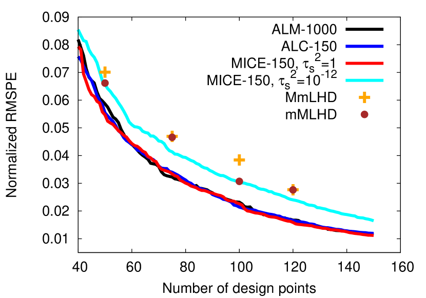
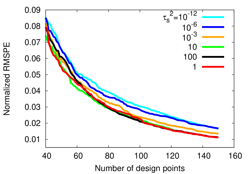
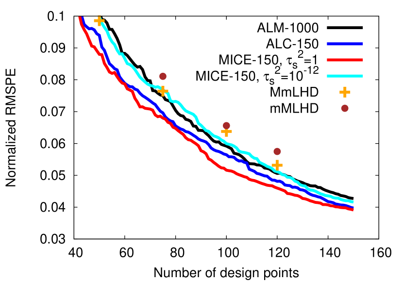
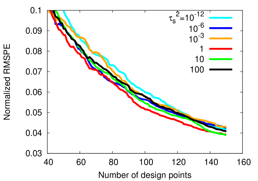
The remaining parameters are specified as Nref=Ncandsubscript𝑁𝑟𝑒𝑓subscript𝑁𝑐𝑎𝑛𝑑N_{ref}=N_{cand} for ALC, as used in [12, 29], and τs2=1subscriptsuperscript𝜏2𝑠1\tau^{2}_{s}=1 for MICE. We have also included results for a range of different choices of τs2subscriptsuperscript𝜏2𝑠\tau^{2}_{s}. In particular, τs2=1012subscriptsuperscript𝜏2𝑠superscript1012\tau^{2}_{s}=10^{-12} which behaves as the MI algorithm, since then τs2τ2subscriptsuperscript𝜏2𝑠superscript𝜏2\tau^{2}_{s}\approx\tau^{2}.

The optimiser employed for the MLE method is a real-coded genetic algorithm [9] with settings that require 1024 calls to the log-likelihood. The values for the uncertain correlation parameters are fixed until the current design is of a specific size (20 if p>𝑝absentp>4, else 10).

5.1 Alan Genz’s Oscillatory function

The “Oscillatory” function belongs to a family of test functions [11] proposed by Alan Genz for the study of quadrature methods. The function is y(𝒙)=cos(𝒄𝒙+2πw),𝒙[0,1]pformulae-sequence𝑦𝒙𝒄𝒙2𝜋𝑤𝒙superscript01𝑝y({\boldsymbol{x}})=\cos\left({\boldsymbol{c}}\cdot{\boldsymbol{x}}+2\pi w\right),\quad{\boldsymbol{x}}\in[0,1]^{p}. The vector 𝒄=(c1,c2,,cp)𝒄subscript𝑐1subscript𝑐2subscript𝑐𝑝{\boldsymbol{c}}=(c_{1},c_{2},\ldots,c_{p}) determines the level of difficulty along the different directions of 𝒳p𝒳superscript𝑝{\mathcal{X}}\subset\mathbb{R}^{p}, and w𝑤w is the displacement. To study the impact of dimension size p𝑝p on the difficulty to predict untried points, 𝒄𝒄{\boldsymbol{c}} is constrained as i=1pci=h,ci>0formulae-sequencesubscriptsuperscript𝑝𝑖1subscript𝑐𝑖subscript𝑐𝑖0\sum^{p}_{i=1}c_{i}=h,c_{i}>0, where hh can be held fixed in order to maintain the difficulty level of the problem for different choices of p𝑝p. Two case examples are considered: 𝒄=(1.85,2.51,1.94,2.70)T𝒄superscript1.852.511.942.70𝑇{\boldsymbol{c}}=(1.85,2.51,1.94,2.70)^{T} and w=0.43𝑤0.43w=0.43 over [0,1]4superscript014[0,1]^{4}, and 𝒄=(0.14,1.69,0.81,1.73,2.10,0.42,0.14,1.97)𝒄0.141.690.811.732.100.420.141.97{\boldsymbol{c}}=(0.14,1.69,0.81,1.73,2.10,0.42,0.14,1.97) and w=0.4𝑤0.4w=0.4 over [0,1]8superscript018[0,1]^{8}, where h=99h=9.

Refer to caption
Refer to caption
Figure 10: Left: comparison between algorithms for the Oscillatory function over [0,1]4superscript014[0,1]^{4}. Right: the performance with MICE-150 for different choices of τs2subscriptsuperscript𝜏2𝑠\tau^{2}_{s}.
Refer to caption
Refer to caption
Figure 11: Left: comparison between algorithms for the Oscillatory function over [0,1]8superscript018[0,1]^{8}. Right: the performance with MICE-150 for different choices of τs2subscriptsuperscript𝜏2𝑠\tau^{2}_{s}.

As can be observed in Figure 10, the sequential designs outperform the ones based on LHDs. As expected, since MmLHD and mMLHD, even if well spaced, do not take into account that y(𝒙)𝑦𝒙y({\boldsymbol{x}}) is anisotropic. The worst performing sequential design is MICE-150 with τs2=1012superscriptsubscript𝜏𝑠2superscript1012\tau_{s}^{2}=10^{-12}, which in fact uses the MI criterion. The poor performance is down to the issue discussed in Section 3.1.2. In the 4-dimensional case, ALM-1000, ALC-150, and MICE-150, produce similar results in terms of prediction error, but as shown in Figure 9, the time to run ALC is significantly higher than for ALM and MICE, which in many cases make it the least favorable, especially if y(𝒙)𝑦𝒙y({\boldsymbol{x}}) is cheaper to evaluate. Even if one assumes that the less costly ALC-50 would produce a similar performance as ALC-150, it would still not be competitive in this case. Observe that τs2=1subscriptsuperscript𝜏2𝑠1\tau^{2}_{s}=1 performs the best.

5.2 Piston simulation function

Here we consider a 7-dimensional example from [2], where the output describes the circular motion of a piston within a cylinder; it obeys the following equations:

y(𝒙)𝑦𝒙\displaystyle y({\boldsymbol{x}}) =2πx1x2+x32x4x5x6x7g1(𝒙), whereabsent2𝜋subscript𝑥1subscript𝑥2superscriptsubscript𝑥32subscript𝑥4subscript𝑥5subscript𝑥6subscript𝑥7subscript𝑔1𝒙 where\displaystyle=2\pi\sqrt{\dfrac{x_{1}}{x_{2}+x_{3}^{2}\frac{x_{4}x_{5}}{x_{6}}\frac{x_{7}}{g_{1}({\boldsymbol{x}})}}},\text{ where} g1(𝒙)subscript𝑔1𝒙\displaystyle g_{1}({\boldsymbol{x}}) =x32x2(g22(𝒙)+4x2x4x5x6x7g2(𝒙))absentsubscript𝑥32subscript𝑥2superscriptsubscript𝑔22𝒙4subscript𝑥2subscript𝑥4subscript𝑥5subscript𝑥6subscript𝑥7subscript𝑔2𝒙\displaystyle=\frac{x_{3}}{2x_{2}}\left(\sqrt{g_{2}^{2}({\boldsymbol{x}})+4x_{2}\frac{x_{4}x_{5}}{x_{6}}x_{7}}-g_{2}({\boldsymbol{x}})\right)
g2(𝒙)subscript𝑔2𝒙\displaystyle g_{2}({\boldsymbol{x}}) =x3x4+19.62x1x2x5x3absentsubscript𝑥3subscript𝑥419.62subscript𝑥1subscript𝑥2subscript𝑥5subscript𝑥3\displaystyle=x_{3}x_{4}+19.62x_{1}-\frac{x_{2}x_{5}}{x_{3}}

Here y(𝒙)𝑦𝒙y({\boldsymbol{x}}) is the cycle time (s) which varies with seven input variables. The design space is given by x1[30,60]subscript𝑥13060x_{1}\in[30,60] (piston weight, kg𝑘𝑔kg), x2[1000,5000]subscript𝑥210005000x_{2}\in[1000,5000] (spring coefficient, N/m𝑁𝑚N/m), x3[0.005,0.020]subscript𝑥30.0050.020x_{3}\in[0.005,0.020] (piston surface area, m2superscript𝑚2m^{2}), x4[90000,110000]subscript𝑥490000110000x_{4}\in[90000,110000] (atmospheric pressure, N/m2𝑁superscript𝑚2N/m^{2}), x5[0.002,0.010]subscript𝑥50.0020.010x_{5}\in[0.002,0.010] (initial gas volume, m3superscript𝑚3m^{3}), x6[340,360]subscript𝑥6340360x_{6}\in[340,360] (filling gas temperature, K) and x7[290,296]subscript𝑥7290296x_{7}\in[290,296] (ambient temperature, K𝐾K). The nonlinearity makes this deterministic computer experiment problem challenging to emulate.
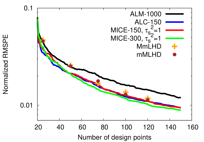
Refer to caption
Refer to caption
Figure 12: Results for the 7-D Piston Simulation function.

MICE-300 yields a slight improvement over MICE-150, see Figure 12. MICE with 300 candidate points is not that much more expensive than with 150; in fact, it is significantly cheaper computationally than ALC with 150. Again, the proposed algorithm MICE performs the best. For high-dimensional problems, ALM tends to be the worst, probably due to the high percentage of points on the boundary.

6 Application to a tsunami simulator

There is a pressing need in tsunami modeling for uncertainty quantification with the specific purpose of providing accurate risk maps or issuing informative warnings. Sarri, Guillas and Dias [27] were the first to demonstrate that statistical emulators can be used for this purpose. Recently, Sraj et al. [32] studied the propagation of uncertainty in Manning’s friction parameterization to the prediction of sea surface elevations, for the Tohoku 2011 tsunami event. They used a polynomial chaos (PC) expansion as the surrogate model of a low resolution tsunami simulator. Note that Bilionis and Zabaras [3] showed that GP emulators can outperform PC expansions when small to moderate-sized training data are considered. Stefanakis et al. [33] used an active experimental design approach for optimization to study if small islands can protect nearby coasts from tsunamis.

We consider here the problem of predicting the maximum free-surface elevation of a tsunami wave at the shoreline, for a wide range of scenarios, following a subaerial landslide at an adjoining beach across a large body of shallow water. A tsunami wave simulator is used. A landslide of seafloor sediments, initially at the beach, has a Gaussian shaped mass distribution, and generates tsunami waves that propagates towards the opposite shoreline across from the beach (see Figure 13). The sea-floor bathymetry is changing over time, and is used as input to the tsunami simulator. The floor motion is described by the change in bathymetry of the sloping beach over time, h(x,t)=H(x)h0(x,t)𝑥𝑡𝐻𝑥subscript0𝑥𝑡h(x,t)=H(x)-h_{0}(x,t), where H(x)=xtanβ𝐻𝑥𝑥𝛽H(x)=x\tan{\beta} is the static uniformly sloping beach, and h0(x,t)=δexp((x~t~)2)subscript0𝑥𝑡𝛿superscript~𝑥~𝑡2h_{0}(x,t)=\delta\exp\left(-(\tilde{x}-\tilde{t})^{2}\right) is the perturbation with respect to H(x,t)𝐻𝑥𝑡H(x,t). Here x~=2xμ2δtanϕ1~𝑥2𝑥superscript𝜇2𝛿subscriptitalic-ϕ1\tilde{x}=2\frac{x\mu^{2}}{\delta\tan{\phi_{1}}}, t~=gδμt~𝑡𝑔𝛿𝜇𝑡\tilde{t}=\sqrt{\frac{g}{\delta}}\mu t, δ𝛿\delta is the maximum vertical slide thickness, μ𝜇\mu is the ratio of the thickness and the slide length, and tanϕ1subscriptitalic-ϕ1\tan{\phi_{1}} is the beach slope. The free surface elevation is defined as z(x,t)=h(x,t)𝑧𝑥𝑡𝑥𝑡z(x,t)=-h(x,t). It is assumed the initial water surface is undisturbed, that is, z(x,0)=0𝑧𝑥00z(x,0)=0 for all x𝑥x. The slope tanϕ2subscriptitalic-ϕ2\tan{\phi_{2}} of the beach at the opposite shoreline is chosen so that the distance between the shorelines is 2800 m. This is a shallow water problem, which means that tanϕ11much-less-thansubscriptitalic-ϕ11\tan{\phi_{1}}\ll 1, and that the translating mass movement is thin (μ=δ/L1𝜇𝛿𝐿much-less-than1\mu=\delta/L\ll 1).

Refer to caption
Figure 13: Case example: landslide-generated tsunami event.

We use the state-of-the-art numerical code VOLNA [10] to simulate all stages of this landslide-generated tsunami event, based on nonlinear shallow water equations. We run VOLNA on a single GPU on the cluster Emerald. The bathymetry defined above is given only along one spatial coordinate, but in the code implementation of VOLNA a second spatial dimension (in this case, along the shoreline) is added to cover 101010 meters of shoreline. The mesh is defined on [5,5]×[0,3000]5503000[-5,5]\times[0,3000] (m2), and consists of 312,016 triangular elements.

We demonstrate the efficiency of the different sequential design methods for the design of a realistic computer experiments. This problem, is inspired by a benchmark problem, given at the Catalina 2004 workshop on long-wave runup models used in the validation of tsunami models. We consider 4 input parameters for emulation: ϕ1[35,70]subscriptitalic-ϕ1superscript35superscript70\phi_{1}\in[35^{\circ},70^{\circ}], ϕ2[35,70]subscriptitalic-ϕ2superscript35superscript70\phi_{2}\in[35^{\circ},70^{\circ}], h[500.0,1000.0]500.01000.0h\in[500.0,1000.0], and μ=[0.01,0.1]𝜇0.010.1\mu=[0.01,0.1].

Refer to caption
Refer to caption
Refer to caption
Refer to caption
Figure 14: Results for a simple tsunami model. Note the log-scale in the lower right figure.

Some of the method-specific parameters are Nref=150subscript𝑁𝑟𝑒𝑓150N_{ref}=150 (ALC) and τs2=1subscriptsuperscript𝜏2𝑠1\tau^{2}_{s}=1 (MICE). Ncand=150subscript𝑁𝑐𝑎𝑛𝑑150N_{cand}=150 is used for ALC and MI, and since ALM is relatively cheap computationally with respect to Ncandsubscript𝑁𝑐𝑎𝑛𝑑N_{cand}, we let Ncand=1000subscript𝑁𝑐𝑎𝑛𝑑1000N_{cand}=1000 for ALM. The results are averages of ten runs. As before, the GPs have a constant mean, and use the Matérn covariance ν=52𝜈52\nu=\frac{5}{2}. A hold-off set of size 500500500 is used to calculate the normalized RMSPE and the maximum error.

In Figure 14 we observe that MICE performs better than ALM and ALC when considering the actual run time. ALM is more competitive when the objective is to minimize the maximum error, since it places most points on the boundary where the largest prediction errors often are located. The maximum prediction errors, over the designs of size 120120120, is 1 meter, or less, in sea surface elevation for waves up to almost 10 meters. Note that in the bottom right figure the total run time is given in logarithmic scale with base 10, and the computational savings are similar-to\sim10-20% by using MICE, or greater if the MLE method were to be applied more sparsely as it dominates the MICE cost. A single run of VOLNA takes on average 850 seconds. The time consumed by the simulator is represented by a gray dashed line in Figure 14 (bottom left figure).

For a more realistic tsunami scenario, with more parameters, the convergence towards a good fit of the GP will be slower. Hence ALC will become relatively much more costly than MICE as ALC’s cost increases steeply with the number of runs. Since each additional run will help gain a lot of precision, we expect that MICE will outperform ALC and ALM even more in such scenarios.

7 Conclusion

In this paper we introduced a new mutual information-based design criterion, MICE, to find a design for good overall prediction in computer experiments. The MICE algorithm is particularly attractive in terms of time complexity of the entire design process. Our numerical studies show that, for a good range of test functions, and a realistic tsunami simulator, MICE is able to outperform popular methods such as ALC, ALM, and LHD. In addition, MICE may outperform the other designs even more (we conjecture around 50-70% more after examining our computational summaries above, depending on the other relative costs) with less frequent updates of the MLE (e.g. every 5-10 steps) of the correlation parameters; this is something to investigate in the future in practical implementations. Our theoretical results also improve our understanding of the nugget parameter on the variance estimation, which is a key ingredient in MICE.

In this article we investigate the computational costs of the algorithms considered. The computational costs of the sequential design algorithms matter when the simulator is neither very cheap (no need for sequential design) nor extremely expensive (the cost of any algorithm is then negligible). This is generally the case in uncertainty quantification studies as models are run at a high fidelity level, but not at their highest level in order to allow the exploration of the input’s influences on the outputs. If the cost of the sequential design algorithm is of the same order of magnitude as the simulator (or say 10-100 times less), then gains can be readily made by running more times the simulator, and more so when the cost of the algorithms increase steeply with design size. Furthermore, it is typical for a research project to be awarded a certain number of hours on a cluster, and thus computational complexity will increase accuracy under the same budget conditions. Another recurrent issue is that clusters are shared among many research projects, often at the local or national level. The queuing time becomes an issue as sometimes there is no cluster configuration that can accommodate the run at the time of job submission. Note that for well parallelized simulators (e.g. climate, fluid dynamics and tsunami models), the queuing time on a busy cluster can be in the order of hours, or days in some instances. By having a performant sequential design strategy, the queuing time can be reduced - sometimes dramatically in case of sudden bottlenecks - by running the simulator less times for the same accuracy.

Finally, further extensions of MICE would be welcome. One such extension would be a MICE algorithm in a non stationary setting, for example, in the treed GP form [12] in which subdomains of the input space, where the input-output relationships are different, are identified, and the sampling is carried out accounting for this behavior. Another possible extension would be to account for multiple outputs in terms of spatial location or behavior. Also, the desire to screen active variables along the sequential design would constitute another extension for models whose large number of variables need to be reduced before, for instance, carrying out uncertainty quantification tasks.

Appendix. Proofs of theorems

Proof. [Theorem 1] Given a GP emulator on Dk=(𝑿k,𝒚k)subscript𝐷𝑘subscript𝑿𝑘subscript𝒚𝑘D_{k}=({\boldsymbol{X}}_{k},{\boldsymbol{y}}_{k}) with constant mean and a fixed correlation matrix with a nugget parameter τ2superscript𝜏2\tau^{2}, the predictive variance for any point 𝒙i𝑿ksubscript𝒙𝑖subscript𝑿𝑘{\boldsymbol{x}}_{i}\in{\boldsymbol{X}}_{k} can be written as:

s^τ22(𝒙i)subscriptsuperscript^𝑠2superscript𝜏2subscript𝒙𝑖\displaystyle\hat{s}^{2}_{\tau^{2}}({\boldsymbol{x}}_{i}) =σ2(1𝒌T(𝒙i))(𝑲+τ2)1𝒌(𝒙i))\displaystyle=\sigma^{2}(1-{\boldsymbol{k}}^{T}({\boldsymbol{x}}_{i}))\left({\boldsymbol{K}}+\tau^{2}\mathcal{I}\right)^{-1}{\boldsymbol{k}}({\boldsymbol{x}}_{i}))
+(1T(𝑲+τ2)1𝒌(𝒙i))1)2/(1T(𝑲+τ2)11)),\displaystyle+(\textbf{1}^{T}({\boldsymbol{K}}+\tau^{2}\mathcal{I})^{-1}{\boldsymbol{k}}({\boldsymbol{x}}_{i}))-1)^{2}/(\textbf{1}^{T}({\boldsymbol{K}}+\tau^{2}\mathcal{I})^{-1}\textbf{1})),

where \mathcal{I} is the k×k𝑘𝑘k\times k identity matrix, then

𝒌T(𝒙i)(𝑲+τ2)1𝒌(𝒙i)superscript𝒌𝑇subscript𝒙𝑖superscript𝑲superscript𝜏21𝒌subscript𝒙𝑖\displaystyle{\boldsymbol{k}}^{T}({\boldsymbol{x}}_{i})\left({\boldsymbol{K}}+\tau^{2}\mathcal{I}\right)^{-1}{\boldsymbol{k}}({\boldsymbol{x}}_{i}) =𝒌T(𝒙i)(𝑲+τ2)1(𝒌(𝒙i)+τ2ei)τ2𝒌T(𝒙i)(𝑲+τ2)1eiabsentsuperscript𝒌𝑇subscript𝒙𝑖superscript𝑲superscript𝜏21𝒌subscript𝒙𝑖superscript𝜏2subscripte𝑖superscript𝜏2superscript𝒌𝑇subscript𝒙𝑖superscript𝑲superscript𝜏21subscripte𝑖\displaystyle={\boldsymbol{k}}^{T}({\boldsymbol{x}}_{i})\left({\boldsymbol{K}}+\tau^{2}\mathcal{I}\right)^{-1}({\boldsymbol{k}}({\boldsymbol{x}}_{i})+\tau^{2}\textbf{e}_{i})-\tau^{2}{\boldsymbol{k}}^{T}({\boldsymbol{x}}_{i})\left({\boldsymbol{K}}+\tau^{2}\mathcal{I}\right)^{-1}\textbf{e}_{i}
=𝒌T(𝒙i)eiτ2𝒌T(𝒙i)(eiT(𝑲+τ2)1)Tabsentsuperscript𝒌𝑇subscript𝒙𝑖subscripte𝑖superscript𝜏2superscript𝒌𝑇subscript𝒙𝑖superscriptsuperscriptsubscripte𝑖𝑇superscript𝑲superscript𝜏21𝑇\displaystyle={\boldsymbol{k}}^{T}({\boldsymbol{x}}_{i})\textbf{e}_{i}-\tau^{2}{\boldsymbol{k}}^{T}({\boldsymbol{x}}_{i})(\textbf{e}_{i}^{T}({\boldsymbol{K}}+\tau^{2}\mathcal{I})^{-1})^{T}
=1τ2𝒌T(𝒙i)(eiT(𝑲+τ2)1)Tabsent1superscript𝜏2superscript𝒌𝑇subscript𝒙𝑖superscriptsuperscriptsubscripte𝑖𝑇superscript𝑲superscript𝜏21𝑇\displaystyle=1-\tau^{2}{\boldsymbol{k}}^{T}({\boldsymbol{x}}_{i})(\textbf{e}_{i}^{T}({\boldsymbol{K}}+\tau^{2}\mathcal{I})^{-1})^{T}
=1τ2eiT(𝑲+τ2)1𝒌(𝒙i)absent1superscript𝜏2superscriptsubscripte𝑖𝑇superscript𝑲superscript𝜏21𝒌subscript𝒙𝑖\displaystyle=1-\tau^{2}\textbf{e}_{i}^{T}({\boldsymbol{K}}+\tau^{2}\mathcal{I})^{-1}{\boldsymbol{k}}({\boldsymbol{x}}_{i})
=1τ2eiT(𝑲+τ2)1(𝒌(𝒙i)+τ2eiτ2ei)absent1superscript𝜏2superscriptsubscripte𝑖𝑇superscript𝑲superscript𝜏21𝒌subscript𝒙𝑖superscript𝜏2subscripte𝑖superscript𝜏2subscripte𝑖\displaystyle=1-\tau^{2}\textbf{e}_{i}^{T}({\boldsymbol{K}}+\tau^{2}\mathcal{I})^{-1}\left({\boldsymbol{k}}({\boldsymbol{x}}_{i})+\tau^{2}\textbf{e}_{i}-\tau^{2}\textbf{e}_{i}\right)
=1τ2+τ4eiT(𝑲+τ2)1ei,absent1superscript𝜏2superscript𝜏4superscriptsubscripte𝑖𝑇superscript𝑲superscript𝜏21subscripte𝑖\displaystyle=1-\tau^{2}+\tau^{4}\textbf{e}_{i}^{T}({\boldsymbol{K}}+\tau^{2}\mathcal{I})^{-1}\textbf{e}_{i},

where eisubscripte𝑖\textbf{e}_{i} is the i𝑖i-th unit vector. Similarly, 1T(𝑲+τ2)1𝒌(𝒙i)=1τ2eiT(𝑲+τ2)11superscript1𝑇superscript𝑲superscript𝜏21𝒌subscript𝒙𝑖1superscript𝜏2superscriptsubscripte𝑖𝑇superscript𝑲superscript𝜏211\textbf{1}^{T}({\boldsymbol{K}}+\tau^{2}\mathcal{I})^{-1}{\boldsymbol{k}}({\boldsymbol{x}}_{i})=1-\tau^{2}\textbf{e}_{i}^{T}({\boldsymbol{K}}+\tau^{2}\mathcal{I})^{-1}\textbf{1}. Insert these results into s^τ22(𝒙i)subscriptsuperscript^𝑠2superscript𝜏2subscript𝒙𝑖\hat{s}^{2}_{\tau^{2}}({\boldsymbol{x}}_{i}), where 𝒙i𝑿ksubscript𝒙𝑖subscript𝑿𝑘{\boldsymbol{x}}_{i}\in{\boldsymbol{X}}_{k}, and we obtain

s^τ22(𝒙i)=σ2(τ2τ4eiT(𝑲+τ2)1ei+τ4(eiT(𝑲+τ2)11)21T(𝑲+τ2)11).subscriptsuperscript^𝑠2superscript𝜏2subscript𝒙𝑖superscript𝜎2superscript𝜏2superscript𝜏4superscriptsubscripte𝑖𝑇superscript𝑲superscript𝜏21subscripte𝑖superscript𝜏4superscriptsuperscriptsubscripte𝑖𝑇superscript𝑲superscript𝜏2112superscript1𝑇superscript𝑲superscript𝜏211\hat{s}^{2}_{\tau^{2}}({\boldsymbol{x}}_{i})=\sigma^{2}\left(\tau^{2}-\tau^{4}\textbf{e}_{i}^{T}({\boldsymbol{K}}+\tau^{2}\mathcal{I})^{-1}\textbf{e}_{i}+\tau^{4}\dfrac{(\textbf{e}_{i}^{T}({\boldsymbol{K}}+\tau^{2}\mathcal{I})^{-1}\textbf{1})^{2}}{\textbf{1}^{T}({\boldsymbol{K}}+\tau^{2}\mathcal{I})^{-1}\textbf{1}}\right).\qquad

Proof. [Theorem 3] Suppose that the design space 𝒳𝒳{\mathcal{X}} is a compact subset of psuperscript𝑝\mathbb{R}^{p}, and discretized into a regular grid 𝑿G𝒳subscript𝑿𝐺𝒳{\boldsymbol{X}}_{G}\subset{\mathcal{X}} with spacing δ>0𝛿0\delta>0. Assume the correlation function K(,)𝐾K(\cdot,\cdot) is Lipschitz continuous, then there exists a constant KL>0subscript𝐾𝐿0K_{L}>0 such that |s^2(𝒙1)s^2(𝒙2)|KL𝒙1𝒙22superscript^𝑠2subscript𝒙1superscript^𝑠2subscript𝒙2subscript𝐾𝐿subscriptnormsubscript𝒙1subscript𝒙22|\hat{s}^{2}({\boldsymbol{x}}_{1})-\hat{s}^{2}({\boldsymbol{x}}_{2})|\leq K_{L}\|{\boldsymbol{x}}_{1}-{\boldsymbol{x}}_{2}\|_{2} for all 𝒙1,𝒙2𝑿Gsubscript𝒙1subscript𝒙2subscript𝑿𝐺{\boldsymbol{x}}_{1},{\boldsymbol{x}}_{2}\in{\boldsymbol{X}}_{G}, where 2\|\cdot\|_{2} is the Euclidean norm. Suppose we have a Gaussian emulator with constant mean, and a non-negative nugget parameter τ2superscript𝜏2\tau^{2}. Then, for any ε>0𝜀0\varepsilon>0, assuming 𝑿Gsubscript𝑿𝐺{\boldsymbol{X}}_{G} has grid spacing δ2ε/(pKL)𝛿2𝜀𝑝subscript𝐾𝐿\delta\leq 2\varepsilon/(\sqrt{p}K_{L}), s^2(𝒙)superscript^𝑠2superscript𝒙\hat{s}^{2}({\boldsymbol{x}}^{*}) is ε𝜀\varepsilon-close to s^2(𝒙n)superscript^𝑠2subscript𝒙𝑛\hat{s}^{2}({\boldsymbol{x}}_{n}) for any untried point 𝒙𝒳superscript𝒙𝒳{\boldsymbol{x}}^{*}\in{\mathcal{X}}, where 𝒙nsubscript𝒙𝑛{\boldsymbol{x}}_{n} is the member of 𝑿Gsubscript𝑿𝐺{\boldsymbol{X}}_{G} closest to 𝒙superscript𝒙{\boldsymbol{x}}^{*}. According to Theorem 1 for any point 𝒙i𝑿Gsubscript𝒙𝑖subscript𝑿𝐺{\boldsymbol{x}}_{i}\in{\boldsymbol{X}}_{G} the predictive variance can be written as:

s^τ22(𝒙i)=σ2(τ2τ4eiT(𝑲+τ2)1ei+τ4(eiT(𝑲+τ2)11)21T(𝑲+τ2)11),subscriptsuperscript^𝑠2superscript𝜏2subscript𝒙𝑖superscript𝜎2superscript𝜏2superscript𝜏4superscriptsubscripte𝑖𝑇superscript𝑲superscript𝜏21subscripte𝑖superscript𝜏4superscriptsuperscriptsubscripte𝑖𝑇superscript𝑲superscript𝜏2112superscript1𝑇superscript𝑲superscript𝜏211\hat{s}^{2}_{\tau^{2}}({\boldsymbol{x}}_{i})=\sigma^{2}\left(\tau^{2}-\tau^{4}\textbf{e}_{i}^{T}({\boldsymbol{K}}+\tau^{2}\mathcal{I})^{-1}\textbf{e}_{i}+\tau^{4}\dfrac{(\textbf{e}_{i}^{T}({\boldsymbol{K}}+\tau^{2}\mathcal{I})^{-1}\textbf{1})^{2}}{\textbf{1}^{T}({\boldsymbol{K}}+\tau^{2}\mathcal{I})^{-1}\textbf{1}}\right),

where \mathcal{I} is the identity matrix, and eisubscripte𝑖\textbf{e}_{i} the i𝑖i-th unit vector. Hence, for any ε>0𝜀0\varepsilon>0 there exists a grid spacing δ>0𝛿0\delta>0 so that σ2τ4b1(τ2)ε<s^τ22(𝒙)σ2τ2<σ2τ4b2(τ2)+εsuperscript𝜎2superscript𝜏4subscript𝑏1superscript𝜏2𝜀subscriptsuperscript^𝑠2superscript𝜏2superscript𝒙superscript𝜎2superscript𝜏2superscript𝜎2superscript𝜏4subscript𝑏2superscript𝜏2𝜀-\sigma^{2}\tau^{4}b_{1}(\tau^{2})-\varepsilon<\hat{s}^{2}_{\tau^{2}}({\boldsymbol{x}}^{*})-\sigma^{2}\tau^{2}<\sigma^{2}\tau^{4}b_{2}(\tau^{2})+\varepsilon, where b1(τ2)=max{eiT(𝑲+τ2)1ei:𝒙i𝑿G}subscript𝑏1superscript𝜏2:superscriptsubscripte𝑖𝑇superscript𝑲superscript𝜏21subscripte𝑖subscript𝒙𝑖subscript𝑿𝐺b_{1}(\tau^{2})=\max\left\{\textbf{e}_{i}^{T}({\boldsymbol{K}}+\tau^{2}\mathcal{I})^{-1}\textbf{e}_{i}:{\boldsymbol{x}}_{i}\in{\boldsymbol{X}}_{G}\right\}, and
b2(τ2)=max{(eiT(𝑲+τ2)11)21T(𝑲+τ2)11:𝒙i𝑿G}subscript𝑏2superscript𝜏2:superscriptsuperscriptsubscripte𝑖𝑇superscript𝑲superscript𝜏2112superscript1𝑇superscript𝑲superscript𝜏211subscript𝒙𝑖subscript𝑿𝐺b_{2}(\tau^{2})=\max\left\{\dfrac{(\textbf{e}_{i}^{T}({\boldsymbol{K}}+\tau^{2}\mathcal{I})^{-1}\textbf{1})^{2}}{\textbf{1}^{T}({\boldsymbol{K}}+\tau^{2}\mathcal{I})^{-1}\textbf{1}}:{\boldsymbol{x}}_{i}\in{\boldsymbol{X}}_{G}\right\}.

Proof. [Theorem 2] This proof follows closely the proof of Lemma 5 and Theorem 7 in [18]. Let us suppose that 𝑿G1𝒳subscript𝑿subscript𝐺1𝒳{\boldsymbol{X}}_{G_{1}}\subset{\mathcal{X}} and 𝑿G2𝒳subscript𝑿subscript𝐺2𝒳{\boldsymbol{X}}_{G_{2}}\subset{\mathcal{X}} are equidistant grids with spacing 2δ2𝛿2\delta, for some δ>0𝛿0\delta>0, and that and that 𝑿G2subscript𝑿subscript𝐺2{\boldsymbol{X}}_{G_{2}} is obtained by translating 𝑿G1subscript𝑿subscript𝐺1{\boldsymbol{X}}_{G_{1}} by distance δ𝛿\delta in Euclidean norm. 𝑿G1subscript𝑿subscript𝐺1{\boldsymbol{X}}_{G_{1}},𝑿G2subscript𝑿subscript𝐺2{\boldsymbol{X}}_{G_{2}} are assumed to cover 𝒳𝒳{\mathcal{X}} in terms of compactness. In the context of experimental design, let us consider 𝑿G1subscript𝑿subscript𝐺1{\boldsymbol{X}}_{G_{1}} to be the set of points available for selection. For a design point 𝒙𝒙{\boldsymbol{x}} in 𝑿G1subscript𝑿subscript𝐺1{\boldsymbol{X}}_{G_{1}}, we denote by 𝒙~~𝒙\tilde{{\boldsymbol{x}}} the corresponding point in 𝑿G2subscript𝑿subscript𝐺2{\boldsymbol{X}}_{G_{2}}, that is, 𝒙𝒙~δ,𝒙𝑿G1formulae-sequencenorm𝒙~𝒙𝛿for-all𝒙subscript𝑿subscript𝐺1\|{\boldsymbol{x}}-\tilde{{\boldsymbol{x}}}\|\geq\delta,\forall{\boldsymbol{x}}\in{\boldsymbol{X}}_{G_{1}}. Let us denote by Y¯1,Y¯2subscript¯𝑌1subscript¯𝑌2\bar{Y}_{1},\bar{Y}_{2} the restriction of the GPs to 𝑿G1,𝑿G2subscript𝑿subscript𝐺1subscript𝑿subscript𝐺2{\boldsymbol{X}}_{G_{1}},{\boldsymbol{X}}_{G_{2}}, respectively, and, for a random variable \cdot in Y¯1subscript¯𝑌1\bar{Y}_{1}, we denote by ~~\tilde{\cdot} the corresponding translated random variable in Y¯2subscript¯𝑌2\bar{Y}_{2}. Also, 𝒳𝒳{\mathcal{X}} is compact and K(,)𝐾K(\cdot,\cdot) is continuous; hence |K(𝒙,𝒙)K(𝒙~,𝒙~)|ε1,𝒙,𝒙𝑿G1formulae-sequence𝐾𝒙superscript𝒙𝐾~𝒙superscript~𝒙subscript𝜀1for-all𝒙superscript𝒙subscript𝑿subscript𝐺1|K({\boldsymbol{x}},{\boldsymbol{x}}^{\prime})-K(\tilde{{\boldsymbol{x}}},\tilde{{\boldsymbol{x}}}^{\prime})|\leq\varepsilon_{1},\forall{\boldsymbol{x}},{\boldsymbol{x}}^{\prime}\in{\boldsymbol{X}}_{G_{1}} (K(,)𝐾K(\cdot,\cdot) uniformly continuous over 𝒳𝒳{\mathcal{X}}). Let 𝑿ksubscript𝑿𝑘{\boldsymbol{X}}_{k} be a subset of 𝑿G1subscript𝑿subscript𝐺1{\boldsymbol{X}}_{G_{1}}. For any 𝒙𝑿G1\𝑿k𝒙\subscript𝑿subscript𝐺1subscript𝑿𝑘{\boldsymbol{x}}\in{\boldsymbol{X}}_{G_{1}}\backslash{\boldsymbol{X}}_{k}, we assume that (𝒙|𝑿k)(𝒙|𝑿k~)conditional𝒙subscript𝑿𝑘conditional𝒙~subscript𝑿𝑘\mathcal{H}({\boldsymbol{x}}|{\boldsymbol{X}}_{k})\geq\mathcal{H}({\boldsymbol{x}}|\tilde{{\boldsymbol{X}}_{k}}) for |𝑿k|2Nsubscript𝑿𝑘2𝑁|{\boldsymbol{X}}_{k}|\leq 2N, which is empirically justified in [18].

Let 𝑿ksubscript𝑿𝑘{\boldsymbol{X}}_{k} be a subset of 𝑿G1subscript𝑿subscript𝐺1{\boldsymbol{X}}_{G_{1}}, and consider a GP on Dk=(𝑿k,𝒚k)subscript𝐷𝑘subscript𝑿𝑘subscript𝒚𝑘D_{k}=({\boldsymbol{X}}_{k},{\boldsymbol{y}}_{k}) with a nugget parameter τ12>0subscriptsuperscript𝜏210\tau^{2}_{1}>0, and a GP emulator on 𝑿G1\𝑿k𝑿G2\subscript𝑿subscript𝐺1subscript𝑿𝑘subscript𝑿subscript𝐺2{\boldsymbol{X}}_{G_{1}}\backslash{\boldsymbol{X}}_{k}\subseteq{\boldsymbol{X}}_{G_{2}} with a nugget τ22>0subscriptsuperscript𝜏220\tau^{2}_{2}>0. First, let us determine an upper bound for |s^k2(𝒙)s^G1\k2(𝒙)|subscriptsuperscript^𝑠2𝑘𝒙subscriptsuperscript^𝑠2\subscript𝐺1𝑘𝒙|\hat{s}^{2}_{k}({\boldsymbol{x}})-\hat{s}^{2}_{G_{1}\backslash k}({\boldsymbol{x}})|:

|s^k2(𝒙)s^G1\k2(𝒙)|=σ2|𝒌kT(𝒙)𝑲k1𝒌k(𝒙)𝒌G1\kT(𝒙)𝑲G1\k1𝒌G1\(𝒙)|subscriptsuperscript^𝑠2𝑘𝒙subscriptsuperscript^𝑠2\subscript𝐺1𝑘𝒙superscript𝜎2subscriptsuperscript𝒌𝑇𝑘𝒙superscriptsubscript𝑲𝑘1subscript𝒌𝑘𝒙subscriptsuperscript𝒌𝑇\subscript𝐺1𝑘𝒙subscriptsuperscript𝑲1\subscript𝐺1𝑘subscript𝒌subscript𝐺1\𝒙\displaystyle|\hat{s}^{2}_{k}({\boldsymbol{x}})-\hat{s}^{2}_{G_{1}\backslash k}({\boldsymbol{x}})|=\sigma^{2}|{\boldsymbol{k}}^{T}_{k}({\boldsymbol{x}}){\boldsymbol{K}}_{k}^{-1}{\boldsymbol{k}}_{k}({\boldsymbol{x}})-{\boldsymbol{k}}^{T}_{G_{1}\backslash k}({\boldsymbol{x}}){\boldsymbol{K}}^{-1}_{G_{1}\backslash k}{\boldsymbol{k}}_{G_{1}\backslash}({\boldsymbol{x}})|
σ2(𝒌kT(𝒙)𝒌G1\kT(𝒙)2𝑲k12(𝒌k(𝒙)2+𝒌G1\k(𝒙)2)\displaystyle\leq\sigma^{2}(\|{\boldsymbol{k}}^{T}_{k}({\boldsymbol{x}})-{\boldsymbol{k}}^{T}_{G_{1}\backslash k}({\boldsymbol{x}})\|_{2}\|{\boldsymbol{K}}^{-1}_{k}\|_{2}(\|{\boldsymbol{k}}_{k}({\boldsymbol{x}})\|_{2}+\|{\boldsymbol{k}}_{G_{1}\backslash k}({\boldsymbol{x}})\|_{2})
+𝒌kT(𝒙)2𝑲k1𝑲G1\k12𝒌G1\kT(𝒙)2)\displaystyle+\|{\boldsymbol{k}}^{T}_{k}({\boldsymbol{x}})\|_{2}\|{\boldsymbol{K}}^{-1}_{k}-{\boldsymbol{K}}^{-1}_{G_{1}\backslash k}\|_{2}\|{\boldsymbol{k}}^{T}_{G_{1}\backslash k}({\boldsymbol{x}})\|_{2})

Since K(,)𝐾K(\cdot,\cdot) is uniformly continuous over 𝒳𝒳{\mathcal{X}}, we know that ε1>0for-allsubscript𝜀10\forall\varepsilon_{1}>0 there exists a spacing δ>0𝛿0\delta>0 such that, for 𝒙𝒙~δnorm𝒙~𝒙𝛿\|{\boldsymbol{x}}-\tilde{{\boldsymbol{x}}}\|\leq\delta, |K(𝒙,𝒙)K(𝒙,𝒙)|ε1𝐾𝒙superscript𝒙𝐾𝒙superscript𝒙subscript𝜀1|K({\boldsymbol{x}},{\boldsymbol{x}}^{\prime})-K({\boldsymbol{x}},{\boldsymbol{x}}^{\prime})|\leq\varepsilon_{1} for 𝒙𝒙𝒙superscript𝒙{\boldsymbol{x}}\neq{\boldsymbol{x}}^{\prime}, and 𝑲k,τ12𝑲G1\k,τ222NNε1+N|τ12τ22|subscriptnormsubscript𝑲𝑘subscriptsuperscript𝜏21subscript𝑲\subscript𝐺1𝑘subscriptsuperscript𝜏222𝑁𝑁subscript𝜀1𝑁subscriptsuperscript𝜏21subscriptsuperscript𝜏22\|{\boldsymbol{K}}_{k,\tau^{2}_{1}}-{\boldsymbol{K}}_{G_{1}\backslash k,\tau^{2}_{2}}\|_{2}\leq\sqrt{N}N\varepsilon_{1}+\sqrt{N}|\tau^{2}_{1}-\tau^{2}_{2}|. We also derive 𝒌kT(𝒙)𝒌G1\kT(𝒙)2ε1Nsubscriptnormsubscriptsuperscript𝒌𝑇𝑘𝒙subscriptsuperscript𝒌𝑇\subscript𝐺1𝑘𝒙2subscript𝜀1𝑁\|{\boldsymbol{k}}^{T}_{k}({\boldsymbol{x}})-{\boldsymbol{k}}^{T}_{G_{1}\backslash k}({\boldsymbol{x}})\|_{2}\leq\varepsilon_{1}\sqrt{N}, and similarly, 𝒌T(𝒙)2CNsubscriptnormsuperscript𝒌𝑇𝒙2𝐶𝑁\|{\boldsymbol{k}}^{T}({\boldsymbol{x}})\|_{2}\leq C\sqrt{N}, where 2\|\cdot\|_{2} is the Euclidean norm, and C=max𝒙𝒳K(𝒙,𝒙)𝐶subscript𝒙𝒳𝐾𝒙𝒙C=\max_{{\boldsymbol{x}}\in{\mathcal{X}}}K({\boldsymbol{x}},{\boldsymbol{x}}). We assume wlog that C=1𝐶1C=1. Furthermore:

𝑲k,τ121𝑲G1\k,τ2212subscriptnormsubscriptsuperscript𝑲1𝑘superscriptsubscript𝜏12subscriptsuperscript𝑲1\subscript𝐺1𝑘superscriptsubscript𝜏222\displaystyle\|{\boldsymbol{K}}^{-1}_{k,\tau_{1}^{2}}-{\boldsymbol{K}}^{-1}_{G_{1}\backslash k,\tau_{2}^{2}}\|_{2} =𝑲k,τ121(𝑲k,τ12𝑲G1\k,τ22)𝑲G1\k,τ2212absentsubscriptnormsubscriptsuperscript𝑲1𝑘subscriptsuperscript𝜏21subscript𝑲𝑘subscriptsuperscript𝜏21subscript𝑲\subscript𝐺1𝑘subscriptsuperscript𝜏22subscriptsuperscript𝑲1\subscript𝐺1𝑘subscriptsuperscript𝜏222\displaystyle=\|{\boldsymbol{K}}^{-1}_{k,\tau^{2}_{1}}({\boldsymbol{K}}_{k,\tau^{2}_{1}}-{\boldsymbol{K}}_{G_{1}\backslash k,\tau^{2}_{2}}){\boldsymbol{K}}^{-1}_{G_{1}\backslash k,\tau^{2}_{2}}\|_{2}
𝑲k,τ1212𝑲k,τ12𝑲G1\k,τ222𝑲G1\k,τ2212absentsubscriptnormsubscriptsuperscript𝑲1𝑘subscriptsuperscript𝜏212subscriptnormsubscript𝑲𝑘subscriptsuperscript𝜏21subscript𝑲\subscript𝐺1𝑘subscriptsuperscript𝜏222subscriptnormsubscriptsuperscript𝑲1\subscript𝐺1𝑘subscriptsuperscript𝜏222\displaystyle\leq\|{\boldsymbol{K}}^{-1}_{k,\tau^{2}_{1}}\|_{2}\|{\boldsymbol{K}}_{k,\tau^{2}_{1}}-{\boldsymbol{K}}_{G_{1}\backslash k,\tau^{2}_{2}}\|_{2}\|{\boldsymbol{K}}^{-1}_{G_{1}\backslash k,\tau^{2}_{2}}\|_{2}
(1+τ12)1(1+τ22)1N(Nε1+|τ12τ22|)NNε1+N|τ12τ22|,absentsuperscript1superscriptsubscript𝜏121superscript1superscriptsubscript𝜏221𝑁𝑁subscript𝜀1superscriptsubscript𝜏12superscriptsubscript𝜏22𝑁𝑁subscript𝜀1𝑁superscriptsubscript𝜏12superscriptsubscript𝜏22\displaystyle\leq(1+\tau_{1}^{2})^{-1}(1+\tau_{2}^{2})^{-1}\sqrt{N}\left(N\varepsilon_{1}+|\tau_{1}^{2}-\tau_{2}^{2}|\right)\leq\sqrt{N}N\varepsilon_{1}+\sqrt{N}|\tau_{1}^{2}-\tau_{2}^{2}|,

where we used that 𝑲𝑲{\boldsymbol{K}} is positive semidefinite, which means that 𝑲12=λmin(𝑲)1(1+τ2)1subscriptnormsuperscript𝑲12subscript𝜆𝑚𝑖𝑛superscript𝑲1superscript1superscript𝜏21\|{\boldsymbol{K}}^{-1}\|_{2}=\lambda_{min}({\boldsymbol{K}})^{-1}\leq(1+\tau^{2})^{-1}, where λmin(𝑲)subscript𝜆𝑚𝑖𝑛𝑲\lambda_{min}({\boldsymbol{K}}) is the smallest eigenvalue. We thus obtain the following bound:

|s^k,τ122(𝒙)s^G1\k,τ222(𝒙)|subscriptsuperscript^𝑠2𝑘subscriptsuperscript𝜏21𝒙subscriptsuperscript^𝑠2\subscript𝐺1𝑘subscriptsuperscript𝜏22𝒙\displaystyle|\hat{s}^{2}_{k,\tau^{2}_{1}}({\boldsymbol{x}})-\hat{s}^{2}_{G_{1}\backslash k,\tau^{2}_{2}}({\boldsymbol{x}})| σ2(2ε1N(1+τ12)1+N(1+τ12)1(1+τ22)1N(Nε1+|τ12τ22|))absentsuperscript𝜎22subscript𝜀1𝑁superscript1superscriptsubscript𝜏121𝑁superscript1superscriptsubscript𝜏121superscript1superscriptsubscript𝜏221𝑁𝑁subscript𝜀1superscriptsubscript𝜏12superscriptsubscript𝜏22\displaystyle\leq\sigma^{2}(2\varepsilon_{1}N(1+\tau_{1}^{2})^{-1}+N(1+\tau_{1}^{2})^{-1}(1+\tau_{2}^{2})^{-1}\sqrt{N}(N\varepsilon_{1}+|\tau_{1}^{2}-\tau_{2}^{2}|))
σ2(2ε1N+NN(Nε1+|τ12τ22|)).absentsuperscript𝜎22subscript𝜀1𝑁𝑁𝑁𝑁subscript𝜀1subscriptsuperscript𝜏21subscriptsuperscript𝜏22\displaystyle\leq\sigma^{2}(2\varepsilon_{1}N+N\sqrt{N}(N\varepsilon_{1}+|\tau^{2}_{1}-\tau^{2}_{2}|)).

Then, for any ε>0𝜀0\varepsilon>0 we can choose the grid spacing δ>0𝛿0\delta>0 such that εε1τ22σ2N(2N+N3/2)𝜀subscript𝜀1superscriptsubscript𝜏22superscript𝜎2𝑁2𝑁superscript𝑁32\varepsilon\geq\varepsilon_{1}\tau_{2}^{2}\sigma^{2}N(2N+N^{3/2}). Hence, |s^k,τ122(𝒙)s^G1\k,τ222(𝒙)|ετ22+σ2N3/2|τ12τ22|subscriptsuperscript^𝑠2𝑘superscriptsubscript𝜏12𝒙subscriptsuperscript^𝑠2\subscript𝐺1𝑘superscriptsubscript𝜏22𝒙𝜀subscriptsuperscript𝜏22superscript𝜎2superscript𝑁32subscriptsuperscript𝜏21subscriptsuperscript𝜏22|\hat{s}^{2}_{k,\tau_{1}^{2}}({\boldsymbol{x}})-\hat{s}^{2}_{G_{1}\backslash k,\tau_{2}^{2}}({\boldsymbol{x}})|\leq\varepsilon\tau^{2}_{2}+\sigma^{2}N^{3/2}|\tau^{2}_{1}-\tau^{2}_{2}|, and, in turn,

τ12(𝒙|𝑿k)τ22(𝒙|𝑿G1\𝑿k)=12log(s^k,τ122(𝒙)s^k,τ222(𝒙))subscriptsubscriptsuperscript𝜏21conditional𝒙subscript𝑿𝑘subscriptsubscriptsuperscript𝜏22conditional𝒙\subscript𝑿subscript𝐺1subscript𝑿𝑘12subscriptsuperscript^𝑠2𝑘subscriptsuperscript𝜏21𝒙subscriptsuperscript^𝑠2𝑘subscriptsuperscript𝜏22𝒙\displaystyle\mathcal{H}_{\tau^{2}_{1}}({\boldsymbol{x}}|{\boldsymbol{X}}_{k})-\mathcal{H}_{\tau^{2}_{2}}({\boldsymbol{x}}|{\boldsymbol{X}}_{G_{1}}\backslash{\boldsymbol{X}}_{k})=\frac{1}{2}\log\left(\frac{\hat{s}^{2}_{k,\tau^{2}_{1}}({\boldsymbol{x}})}{\hat{s}^{2}_{k,\tau^{2}_{2}}({\boldsymbol{x}})}\right)
=12log(1+(s^k,τ122(𝒙)s^G\k,τ222(𝒙))/s^G1\k,τ222(𝒙))absent121subscriptsuperscript^𝑠2𝑘subscriptsuperscript𝜏21𝒙subscriptsuperscript^𝑠2\𝐺𝑘subscriptsuperscript𝜏22𝒙subscriptsuperscript^𝑠2\subscript𝐺1𝑘subscriptsuperscript𝜏22𝒙\displaystyle=\frac{1}{2}\log\left(1+(\hat{s}^{2}_{k,\tau^{2}_{1}}({\boldsymbol{x}})-\hat{s}^{2}_{G\backslash k,\tau^{2}_{2}}({\boldsymbol{x}}))/\hat{s}^{2}_{G_{1}\backslash k,\tau^{2}_{2}}({\boldsymbol{x}})\right)
12log(1+ε+N5/2|τ12τ22|/τ22)ε+N5/2|τ22τ12|/τ22.absent121𝜀superscript𝑁52superscriptsubscript𝜏12superscriptsubscript𝜏22subscriptsuperscript𝜏22𝜀superscript𝑁52superscriptsubscript𝜏22superscriptsubscript𝜏12subscriptsuperscript𝜏22\displaystyle\leq\frac{1}{2}\log\left(1+\varepsilon+N^{5/2}|\tau_{1}^{2}-\tau_{2}^{2}|/\tau^{2}_{2}\right)\leq\varepsilon+N^{5/2}|\tau_{2}^{2}-\tau_{1}^{2}|/\tau^{2}_{2}.

We used that s^G1\k2(𝒙)σ2τ22/Nsubscriptsuperscript^𝑠2\subscript𝐺1𝑘𝒙superscript𝜎2superscriptsubscript𝜏22𝑁\hat{s}^{2}_{G_{1}\backslash k}({\boldsymbol{x}})\geq\sigma^{2}\tau_{2}^{2}/N (see Theorem 1). Suppose that estimates are available for the correlation parameters 𝝃𝝃{\boldsymbol{\xi}}; replacing K(𝒙,𝒙)𝐾𝒙𝒙K({\boldsymbol{x}},{\boldsymbol{x}}) by K(𝒙,𝒙;𝝃^)𝐾𝒙superscript𝒙^𝝃K({\boldsymbol{x}},{\boldsymbol{x}}^{\prime};\hat{{\boldsymbol{\xi}}}) throughout the calculations above. Then, an extra term is added to s^2(𝒙)superscript^𝑠2𝒙\hat{s}^{2}({\boldsymbol{x}}) to account for the parameter uncertainty [35]: s^2(𝒙;𝝃^)=σ2(1𝒌T(𝒙;𝝃^i)𝑲𝝃^i1𝒌(𝒙;𝝃^i))+E((y^(𝒙;𝝃)y^(𝒙;𝝃^i))2)superscript^𝑠2𝒙^𝝃superscript𝜎21superscript𝒌𝑇𝒙subscript^𝝃𝑖superscriptsubscript𝑲subscript^𝝃𝑖1𝒌𝒙subscript^𝝃𝑖𝐸superscript^𝑦𝒙𝝃^𝑦𝒙subscript^𝝃𝑖2\hat{s}^{2}({\boldsymbol{x}};\hat{{\boldsymbol{\xi}}})=\sigma^{2}(1-{\boldsymbol{k}}^{T}({\boldsymbol{x}};\hat{{\boldsymbol{\xi}}}_{i}){\boldsymbol{K}}_{\hat{{\boldsymbol{\xi}}}_{i}}^{-1}{\boldsymbol{k}}({\boldsymbol{x}};\hat{{\boldsymbol{\xi}}}_{i}))+E\left((\hat{y}({\boldsymbol{x}};{\boldsymbol{\xi}})-\hat{y}({\boldsymbol{x}};\hat{{\boldsymbol{\xi}}}_{i}))^{2}\right). The estimates are updated at each greedy step, denoted by 𝝃^isubscript^𝝃𝑖\hat{{\boldsymbol{\xi}}}_{i}, for greedy step i𝑖i. Using Eq. (4), with zero-mean, y^(𝒙;𝝃)y^(𝒙;𝝃^i)=𝒌𝝃T(𝒙)𝑲𝝃1𝒚k𝒌𝝃^iT(𝒙)𝑲𝝃^i1𝒚k^𝑦𝒙𝝃^𝑦𝒙subscript^𝝃𝑖subscriptsuperscript𝒌𝑇𝝃𝒙superscriptsubscript𝑲𝝃1subscript𝒚𝑘subscriptsuperscript𝒌𝑇subscript^𝝃𝑖𝒙superscriptsubscript𝑲subscript^𝝃𝑖1subscript𝒚𝑘\hat{y}({\boldsymbol{x}};{\boldsymbol{\xi}})-\hat{y}({\boldsymbol{x}};\hat{{\boldsymbol{\xi}}}_{i})={\boldsymbol{k}}^{T}_{{\boldsymbol{\xi}}}({\boldsymbol{x}}){\boldsymbol{K}}_{{\boldsymbol{\xi}}}^{-1}{\boldsymbol{y}}_{k}-{\boldsymbol{k}}^{T}_{\hat{{\boldsymbol{\xi}}}_{i}}({\boldsymbol{x}}){\boldsymbol{K}}_{\hat{{\boldsymbol{\xi}}}_{i}}^{-1}{\boldsymbol{y}}_{k}. Let us assume that 𝒚k2Nsubscriptnormsubscript𝒚𝑘2𝑁\|{\boldsymbol{y}}_{k}\|_{2}\leq\sqrt{N} (normalized). We know that there exists a constant α0𝛼0\alpha\geq 0 such that, for all {𝝃^i}i=1ksubscriptsuperscriptsubscript^𝝃𝑖𝑘𝑖1\{\hat{{\boldsymbol{\xi}}}_{i}\}^{k}_{i=1}, and for all, 𝒙,𝒙𝒳,|K(𝒙,𝒙;𝝃)K(𝒙,𝒙;𝝃^i)|αformulae-sequence𝒙superscript𝒙𝒳𝐾𝒙superscript𝒙𝝃𝐾𝒙superscript𝒙subscript^𝝃𝑖𝛼{\boldsymbol{x}},{\boldsymbol{x}}^{\prime}\in{\mathcal{X}},|K({\boldsymbol{x}},{\boldsymbol{x}}^{\prime};{\boldsymbol{\xi}})-K({\boldsymbol{x}},{\boldsymbol{x}}^{\prime};\hat{{\boldsymbol{\xi}}}_{i})|\leq\alpha. Then, E(y^(𝒙;𝝃^i)(y^(𝒙;𝝃))2)=E((𝒌𝝃^iT(𝒙)𝑲𝝃^i1𝒚k𝒌𝝃T(𝒙)𝑲𝝃1𝒚k)2)E((𝒌𝝃T(𝒙)𝒌𝝃^iT(𝒙)2𝑲𝝃^i12𝒚k2+𝒌𝝃^iT(𝒙)2𝑲𝝃1𝑲𝝃^i12)𝒚k2)2)α2N2(1+N3/2)2E(\hat{y}({\boldsymbol{x}};\hat{{\boldsymbol{\xi}}}_{i})-(\hat{y}({\boldsymbol{x}};{\boldsymbol{\xi}}))^{2})=E(({\boldsymbol{k}}^{T}_{\hat{{\boldsymbol{\xi}}}_{i}}({\boldsymbol{x}}){\boldsymbol{K}}_{\hat{{\boldsymbol{\xi}}}_{i}}^{-1}{\boldsymbol{y}}_{k}-{\boldsymbol{k}}^{T}_{{\boldsymbol{\xi}}}({\boldsymbol{x}}){\boldsymbol{K}}_{{\boldsymbol{\xi}}}^{-1}{\boldsymbol{y}}_{k})^{2})\leq E((\|{\boldsymbol{k}}^{T}_{{\boldsymbol{\xi}}}({\boldsymbol{x}})-{\boldsymbol{k}}^{T}_{\hat{{\boldsymbol{\xi}}}_{i}}({\boldsymbol{x}})\|_{2}\|{\boldsymbol{K}}_{\hat{{\boldsymbol{\xi}}}_{i}}^{-1}\|_{2}\|{\boldsymbol{y}}_{k}\|_{2}+\|{\boldsymbol{k}}_{\hat{{\boldsymbol{\xi}}}_{i}}^{T}({\boldsymbol{x}})\|_{2}\|{\boldsymbol{K}}^{-1}_{{\boldsymbol{\xi}}}-{\boldsymbol{K}}^{-1}_{\hat{{\boldsymbol{\xi}}}_{i}}\|_{2})\|{\boldsymbol{y}}_{k}\|_{2})^{2})\leq\alpha^{2}N^{2}(1+N^{3/2})^{2}. As a result, using similar calculations, (𝒙|k)(𝒙|k,𝝃^)12log((s^k2(𝒙)+α2N2(1+N3/2)2)/s^D2(𝒙))12log(1+(ασ1τ1)2N3(1+N3/2)2)conditional𝒙𝑘conditional𝒙𝑘^𝝃12superscriptsubscript^𝑠𝑘2𝒙superscript𝛼2superscript𝑁2superscript1superscript𝑁322superscriptsubscript^𝑠𝐷2𝒙121superscript𝛼superscript𝜎1superscript𝜏12superscript𝑁3superscript1superscript𝑁322\mathcal{H}({\boldsymbol{x}}|k)-\mathcal{H}({\boldsymbol{x}}|k,\hat{{\boldsymbol{\xi}}})\leq\frac{1}{2}\log((\hat{s}_{k}^{2}({\boldsymbol{x}})+\alpha^{2}N^{2}(1+N^{3/2})^{2})/\hat{s}_{D}^{2}({\boldsymbol{x}}))\leq\frac{1}{2}\log(1+(\alpha\sigma^{-1}\tau^{-1})^{2}N^{3}(1+N^{3/2})^{2}). Hence,

(𝒙|k,ξ^,τ12)(𝒙|(𝑿G1\𝑿k),ξ^,τ22)=((𝒙|k,τ12)(𝒙|(𝑿G1\𝑿k),τ12))conditional𝒙𝑘^𝜉superscriptsubscript𝜏12conditional𝒙\subscript𝑿subscript𝐺1subscript𝑿𝑘^𝜉superscriptsubscript𝜏22conditional𝒙𝑘superscriptsubscript𝜏12conditional𝒙\subscript𝑿subscript𝐺1subscript𝑿𝑘superscriptsubscript𝜏12\displaystyle\mathcal{H}({\boldsymbol{x}}|k,\hat{\xi},\tau_{1}^{2})-\mathcal{H}({\boldsymbol{x}}|({\boldsymbol{X}}_{G_{1}}\backslash{\boldsymbol{X}}_{k}),\hat{\xi},\tau_{2}^{2})=(\mathcal{H}({\boldsymbol{x}}|k,\tau_{1}^{2})-\mathcal{H}({\boldsymbol{x}}|({\boldsymbol{X}}_{G_{1}}\backslash{\boldsymbol{X}}_{k}),\tau_{1}^{2}))
+((𝒙|(𝑿G1\𝑿k),τ12)(𝒙|(𝑿G1\𝑿k),ξ^,τ12))+((𝒙|k,ξ^,τ12)(𝒙|k,τ12))conditional𝒙\subscript𝑿subscript𝐺1subscript𝑿𝑘superscriptsubscript𝜏12conditional𝒙\subscript𝑿subscript𝐺1subscript𝑿𝑘^𝜉superscriptsubscript𝜏12conditional𝒙𝑘^𝜉superscriptsubscript𝜏12conditional𝒙𝑘superscriptsubscript𝜏12\displaystyle+(\mathcal{H}({\boldsymbol{x}}|({\boldsymbol{X}}_{G_{1}}\backslash{\boldsymbol{X}}_{k}),\tau_{1}^{2})-\mathcal{H}({\boldsymbol{x}}|({\boldsymbol{X}}_{G_{1}}\backslash{\boldsymbol{X}}_{k}),\hat{\xi},\tau_{1}^{2}))+(\mathcal{H}({\boldsymbol{x}}|k,\hat{\xi},\tau_{1}^{2})-\mathcal{H}({\boldsymbol{x}}|k,\tau_{1}^{2}))
+((𝒙|(𝑿G1\𝑿k),ξ^,τ12)(𝒙|(𝑿G1\𝑿k),ξ^,τ22))conditional𝒙\subscript𝑿subscript𝐺1subscript𝑿𝑘^𝜉superscriptsubscript𝜏12conditional𝒙\subscript𝑿subscript𝐺1subscript𝑿𝑘^𝜉superscriptsubscript𝜏22\displaystyle+(\mathcal{H}({\boldsymbol{x}}|({\boldsymbol{X}}_{G_{1}}\backslash{\boldsymbol{X}}_{k}),\hat{\xi},\tau_{1}^{2})-\mathcal{H}({\boldsymbol{x}}|({\boldsymbol{X}}_{G_{1}}\backslash{\boldsymbol{X}}_{k}),\hat{\xi},\tau_{2}^{2}))
ε+2(ασ1τ1)2N3(1+N3/2)2+N5/2|τ22τ12|/τ22.absent𝜀2superscript𝛼superscript𝜎1superscript𝜏12superscript𝑁3superscript1superscript𝑁322superscript𝑁52superscriptsubscript𝜏22superscriptsubscript𝜏12subscriptsuperscript𝜏22\displaystyle\leq\varepsilon+2(\alpha\sigma^{-1}\tau^{-1})^{2}N^{3}(1+N^{3/2})^{2}+N^{5/2}|\tau_{2}^{2}-\tau_{1}^{2}|/\tau^{2}_{2}.

The two GPs on 𝑿ksubscript𝑿𝑘{\boldsymbol{X}}_{k} and 𝑿G1\𝑿k\subscript𝑿subscript𝐺1subscript𝑿𝑘{\boldsymbol{X}}_{G_{1}}\backslash{\boldsymbol{X}}_{k}, respectively, use the same estimates 𝝃^^𝝃\hat{{\boldsymbol{\xi}}}. Finally, by following the same the proof of Theorem 7 in [18], we can easily get the result of this theorem.

Acknowledgments

This research was part funded by the NERC research programme “Probability, Uncertainty and Risk in the Environment” (PURE), grant NE/J017434/1. The authors would like to acknowledge that the work presented here made use of the Emerald High Performance Computing facility made available by the Centre for Innovation. The Centre is formed by the universities of Oxford, Southampton, Bristol, and University College London in partnership with the STFC Rutherford-Appleton Laboratory.

References

  • [1] S Ba and VR Joseph. Multi-layer designs for computer experiments. J Am Stat Assoc, 106(495), 2011.
  • [2] EN Ben-Ari and DM Steinberg. Modeling data from computer experiments: an empirical comparison of kriging with MARS and projection pursuit regression. Qual Eng, 19(4):327–338, 2007.
  • [3] I Bilionis and N Zabaras. Multi-output local Gaussian process regression: Applications to uncertainty quantification. J Comput Phys, 231(17):5718–5746, 2012.
  • [4] WF Caselton and JV Zidek. Optimal monitoring network designs. Stat Probabil Lett, 2(4):223–227, 1984.
  • [5] JA Christen and B Sansó. Advances in the sequential design of computer experiments based on active learning. Commun Stat A-Theor, 40(24):4467–4483, 2011.
  • [6] E Contal, V Perchet, and N Vayatis. Gaussian process optimization with mutual information. In 31st Proc. ICML, pages 253–261, 2014.
  • [7] TM Cover and JA Thomas. Elements of information theory. Wiley Series in Telecommunications and Signal Processing. Wiley-Interscience, 2 edition, 2006.
  • [8] C Currin, TJ Mitchell, MD Morris, and D Ylvisaker. A Bayesian approach to the design and analysis of computer experiments. Technical Report ORNL-6498, available from National Technical Information Service, 5285 Port Royal Road, Springfield, VA 22161, 1988.
  • [9] K Deb and RB Agrawal. Simulated binary crossover for continuous search space. Complex Syst, 9(2):115–148, 1995.
  • [10] D Dutykh, R Poncet, and F Dias. The VOLNA code for the numerical modeling of tsunami waves: Generation, propagation and inundation. Eur J Mech B-Fluid, 30(6):598–615, 2011.
  • [11] A Genz. An adaptive numerical integration algorithm for simplices. In Computing in the 90’s, pages 279–285. Springer, 1991.
  • [12] RB Gramacy and HKH Lee. Adaptive design and analysis of supercomputer experiments. Technometrics, 51(2), 2009.
  • [13] RB Gramacy and HKH Lee. Cases for the nugget in modeling computer experiments. Stat Comp, 22(3):713–722, 2012.
  • [14] MS Handcock and ML Stein. A Bayesian analysis of kriging. Technometrics, 35(4):403–410, 1993.
  • [15] X Huan and YM Marzouk. Simulation-based optimal bayesian experimental design for nonlinear systems. J Comput Phys, 232(1):288–317, 2013.
  • [16] DR Jones. A taxonomy of global optimization methods based on response surfaces. J Global Optim, 21(4):345–383, 2001.
  • [17] CW Ko, J Lee, and M Queyranne. An exact algorithm for maximum entropy sampling. Oper Res, 43(4):684–691, 1995.
  • [18] A Krause, A Singh, and C Guestrin. Near-optimal sensor placements in Gaussian processes: Theory, efficient algorithms and empirical studies. J Mach Learn Res, 9:235–284, 2008.
  • [19] AM Kupresanin and G Johannesson. Comparison of sequential designs of computer experiments in high dimensions. Technical Report LLNL-TR-491692, Lawrence Livermore National Laboratory (LLNL), Livermore, CA, 2011.
  • [20] CQ Lam and WI Notz. Sequential adaptive designs in computer experiments for response surface model fit. Stat Appl, 6(1-2):207–233, 2008.
  • [21] DV Lindley. On a measure of the information provided by an experiment. Ann Math Stat, pages 986–1005, 1956.
  • [22] GL Nemhauser, LA Wolsey, and ML Fisher. An analysis of approximations for maximizing submodular set functions. Math Program, 14(1):265–294, 1978.
  • [23] C Rasmussen and C Williams. Gaussian processes for machine learning. MIT Press, 2006.
  • [24] GK Robinson. That BLUP is a good thing: the estimation of random effects. Stat Sci, pages 15–32, 1991.
  • [25] J Sacks, WJ Welch, TJ Mitchell, and HP Wynn. Design and analysis of computer experiments. Stat Sci, 4(4):409–423, 1989.
  • [26] TJ Santner, BJ Williams, and WI Notz. The design and analysis of computer experiments. Springer Verlag, New York, 2003.
  • [27] A Sarri, S Guillas, and F Dias. Statistical emulation of a tsunami model for sensitivity analysis and uncertainty quantification. Nat Hazards Earth Syst Sci, 12:2003–2018, 2012.
  • [28] M Schonlau. Computer experiments and global optimization. PhD thesis, University of Waterloo, 1998.
  • [29] S Seo, M Wallat, T Graepel, and K Obermayer. Gaussian process regression: Active data selection and test point rejection. In IEEE-IJCNN, volume 3, pages 241–246, 2000.
  • [30] MC Shewry and HP Wynn. Maximum entropy sampling. J Appl Stat, 14(2):165–170, 1987.
  • [31] TW Simpson, DKJ Lin, and W Chen. Sampling strategies for computer experiments: design and analysis. Int J Reliab Appl, 2(3):209–240, 2001.
  • [32] I Sraj, KT Mandli, OM Knio, CN Dawson, and I Hoteit. Uncertainty quantification and inference of Manning’s friction coefficients using DART buoy data during the tōhoku tsunami. Ocean Model, 83:82–97, 2014.
  • [33] TS Stefanakis, E Contal, N Vayatis, F Dias, and CE Synolakis. Can small islands protect nearby coasts from tsunamis? an active experimental design approach. Philos T Roy Soc A, 470(2172):1–20, 2014.
  • [34] ML Stein. Interpolation of spatial data: Some theory for kriging. Springer Verlag, New York, 1999.
  • [35] DL Zimmerman and N Cressie. Mean squared prediction error in the spatial linear model with estimated covariance parameters. Ann Inst Statist Math, 44(1):27–43, 1992.