Correlated percolation models of structured habitat in ecology
Abstract
Percolation offers acknowledged models of random media when the relevant medium characteristics can be described as a binary feature. However, when considering habitat modeling in ecology, a natural constraint comes from nearest-neighbor correlations between the suitable/unsuitable states of the spatial units forming the habitat. Such constraints are also relevant in the physics of aggregation where underlying processes may lead to a form of correlated percolation. However, in ecology, the processes leading to habitat correlations are in general not known or very complex. As proposed by Hiebeler [Ecology 81, 1629 (2000)], these correlations can be captured in a lattice model by an observable aggregation parameter , supplementing the density of suitable sites. We investigate this model as an instance of correlated percolation. We analyze the phase diagram of the percolation transition and compute the cluster size distribution, the pair-connectedness function and the correlation function . We find that while displays a power-law decrease associated with long-range correlations in a wide domain of parameter values, critical properties are compatible with the universality class of uncorrelated percolation. We contrast the correlation structures obtained respectively for the correlated percolation model and for the Ising model, and show that the diversity of habitat configurations generated by the Hiebeler model is richer than the archetypal Ising model. We also find that emergent structural properties are peculiar to the implemented algorithm, leading to questioning the notion of a well-defined model of aggregated habitat. We conclude that the choice of model and algorithm have strong consequences on what insights ecological studies can get using such models of species habitat.
1 Introduction
Much research in ecology is devoted to investigating the dynamics of organisms in space and time, according to their survival, reproduction and dispersal abilities. A challenging issue is to characterize these dynamics under the constraint of a spatially heterogeneous environment, such that some sites allow successful establishment or survival while others do not. The habitat can then be seen as the ensemble of suitable sites, located on a discretized lattice; the other sites being defined as unsuitable, and a priori forbidden to the organism. Ecologists aim at describing the main spatial properties of this habitat based on a minimal number of parameters. They have mainly considered characterizing habitat structure based on its spatial autocorrelation. This focus is related to the fact that: (i) the habitat is generated by other organisms that exhibit diffusive dynamics and aggregated patterns (e.g., a forested vegetation pattern), (ii) an organism that live and move in this habitat has itself limited ability to disperse far away from the sources (e.g. a bird living in the forested vegetation), and thereby also exhibit aggregated spatial structures. In this regard, Hiebeler [12] proposed a model of habitat structure based on a parameter of density, , the proportion of suitable sites in the lattice, and a parameter of aggregation, , the probability to find a suitable site nearby another suitable one. A crucial ingredient of the model is the algorithm that constructs habitat maps with target parameters . An overlooked issue in ecology is whether such a convenient and reduced set of parameters allows characterizing any habitat spatial structure in an unambiguous way. We will show that the answer is clearly no, and the habitat characteristics depend dramatically on the algorithm specifications.The parameterization, as well as other versions using longer-range parameters of correlation, are in fact based on an implicit process of habitat generation resulting in the aggregated pattern. But algorithms used to simulate habitats for these parameters perform ad hoc switches of suitable site labels in order to converge to the expected spatial structure. Here we question whether such algorithms based on expected patterns rather than on underlying generating mechanisms allow getting a well-defined typology of habitat, or alternatively generate different results according to the generating algorithm. Whether or not the habitat is defined in an unambiguous way is indeed critical to the analysis of organism dynamics within this habitat.
Percolation theory is one of the most important landmarks in statistical physics, in relation with the theory of critical phenomena. The basic percolation model, namely uncorrelated site percolation, only prescribes habitat density , such as each site is suitable independently from the other sites. The model displays a critical transition at a value , above which the lattice is spanned by an infinite cluster (connected set) of suitable sites. The threshold value has been determined for a variety of infinite lattices, with in a square lattice [1]. Models of correlated percolation conversely consider that the probability of a site being suitable depends on the status of its neighbors [25]. Another archetypal model of statistical physics, the Ising model, is based on local particle interactions resulting in patterns of spatially correlated structures [28, 29]. The spatial properties of this model are well-known and can thereby serve as a reference to understand the structure of correlated habitat. However the magnetic field and the interaction parameter of the Ising model are very difficult to calibrate in the context of an ecological habitat depending on many underlying dynamical processes. That is why ecologists have still resorted to describe habitats based on resulting habitat structure rather than based on generating mechanisms. We therefore wish to assess the relationship between models of correlated percolation of physics with the models of correlated habitat of ecologists. We focus on correlated percolation models prescribed by local rules, namely correlations between nearest neighbors, to comply with the minimal parameterization of Hiebeler.
The Hiebeler model is hence a new model of correlated percolation that has never been investigated in the past in the light of statistical physics. Such a model could also be of interest in materials physics for the design of porous media for instance [3]. We will show that the choice of the parameterization, though appealing for ecologists, is not unequivocal and that the consequences are critical for the understanding of organism spatial dynamics in structured habitats. Our demonstration is based on a comparison of the properties of the Hiebeler model with the Ising model, and on an assessment of the sensitivity of these properties to algorithmic choices. In Section II, we formulate in physical terms the nearest-neighbor model of aggregation introduced on ecological grounds by Hiebeler [12]. Section III is devoted to the analysis of the Hiebeler model in the light of statistical physics and percolation theory. We investigate its phase diagram and compute its spatial properties. In Section IV we show that a mapping is possible between the Hiebeler model and Ising model, though being incomplete and sometimes equivocal. This allows highlighting differences between the two models, the Hiebeler model showing more diversity in configuration space that its physical counterpart. In Section V, we discuss the relevance of the Hiebeler model for modeling ecological habitats. In particular we discuss how dynamical models with local dispersion rules can be most conveniently studied on a Hiebeler type of habitat, with the aggregation parameter being the fundamental quantity necessary to assess the survival of organisms on such substrates.
2 The nearest-neighbor aggregation model of Hiebeler
2.1 Pairwise conditional probabilities
The first prescription of the model is an homogeneous probability of site suitability:
| (1) |
where labels the sites of a square lattice and is the Boolean random variable describing the status of the site : if the site is suitable, otherwise . In contrast to uncorrelated percolation, the suitability of sites is now correlated according to the prescription of conditional probabilities between nearest neighbors:
| (2) |
for any . is termed the aggregation parameter. It is straightforward to derive the other nearest-neighbor conditional probabilities, in particular
| (3) |
Requiring the non-negativity of this probability yields the following condition
| (4) |
Therefore, when considering the behavior of the model at varying (,) values, the region defined by will be an excluded region [13].
Based only on these constraints, the model does not prescribe all the moments of the state variable , nor even the second moment for any pair of sites. Both spatial and statistical closures are required to get a full knowledge of the global distribution.
2.2 Hiebeler’s algorithm and some alternatives
Given the parameters and , the algorithm proposed by Hiebeler [13] for generating binary configurations of suitable/unsuitable habitat on a square lattice proceeds in two steps. In the first step, each site of the lattice is labelled suitable with a probability independently of the other sites. In the second step, a site is chosen at random and its state is switched if this change induces a reduction in the difference between the desired and the observed () joint probabilities, measured via the following cost function :
| (5) |
where the sum runs over the pairs of nearest neighbors, and over states and taking the values or . This step is applied repeatedly, until a given maximum number of iterations is achieved, or when the difference between the desired and observed probabilities reaches a low-enough predetermined threshold (we chose the default threshold equal to 0.001 as used in [13]). This procedure implies that the final values of both and can be slightly different from their target values. As mentioned in [13], the convergence is hard to achieve for some pairs , typically in the situation of low suitable habitat and large clustering ( small and large). In this case, the difference between the initial and the desired values of the parameters is typically larger than in other regions of parameter space.
An important question raised by this algorithm is to understand to what extent the local prescriptions and control the overall spatial structure of the simulated habitat. To investigate this question, we compared Hiebeler’s algorithm with two other methods in order to determine whether some implicit constraint in the algorithm affects the global properties of the system. For these two alternative algorithms, the first step is still the same and consists in a random independent filling of the lattice sites with the probability . In a first variant, one picks randomly a pair of sites (instead of randomly picking one site in the lattice) and tries to exchange their suitability values. If this exchange reduces the value of the cost function the new configuration is accepted, otherwise one picks another pair of sites, until reaches the threshold value. In this procedure, the density of suitable sites remains constant. This algorithm was already proposed in [14]. The second variant consists in picking only pairs of neighboring sites, instead of any pair of sites on the lattice. In both variants the convergence is speeded up. Another variant was proposed by Hiebeler in [15], but the convergence of the algorithm remains slow for some range of parameters. The following Section III presents how the global properties of the model are sensitive to such changes in the algorithm.
3 Percolation transition and correlation properties of the Hiebeler model
We used Hiebeler’s algorithm and the alternative algorithms presented above to simulate matrices of binary habitats of size 10001000. This choice of corresponds to a compromise between long computation times for large lattices and a more important variability between runs for smaller lattice sizes. The results were checked and confirmed by implementing simulation with a larger lattice of size 25002500 when it was tractable. In several cases where finite-size effects were too large to give reliable results, especially for estimating critical exponents, we also performed simulation on 1000010000 lattices. Unless explicitly mentioned, results presented below are based on the original Hiebeler’s algorithm with .
3.1 Percolation transition and phase diagram
3.1.1 Zero-one percolation transition
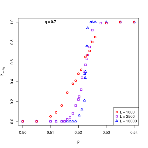
A zero-one behavior has been demonstrated in the case of uncorrelated percolation, stating that either almost all or almost none of the configurations of the square lattice percolate, according to the value of [16]. The mathematical proof is based on the fact that the existence of an infinite cluster is a tail event, that is, it is not affected by a change in the state of a finite number of cells. Hence, the standard zero-one law for uncorrelated sequences of random variables (here, the binary variables describing cells suitability) ensures that the probability of this event is either 0 or 1 [17]. However, the extension of the zero-one law to correlated sequences of random variables is not straightforward [18]. Computing the probability that a configuration contains a spanning cluster as a function of at fixed and increasing numerically supports an all-or-none behavior in infinite lattices (Fig. 1). Although this result has not the status of a rigorous mathematical proof, it gives a strong clue that a zero-one law holds in the case of correlated percolation. We underline here that is a probability in the space of lattice configurations. Accordingly, a zero-one behavior would ensure that almost all configurations (for ) or almost none (for ) percolate. This typicality of individual realizations is a pre-requisite to a numerical study, since it makes possible to detect a bona fide transition on a single realization of the system.
3.1.2 Percolation probability
By analogy with uncorrelated percolation, the order parameter of correlated percolation is the percolation probability , defined as the fraction of sites belonging to the infinite cluster (equal to 0 when there is no infinite cluster). In the case of uncorrelated percolation, percolation probability obeys a scaling law above the threshold, and . The associated exponent is universal insofar as it depends only on the dimension, but not on the geometry of the lattice, in contrast to the lattice-dependent threshold value . Percolation probability should not be confused with the above-mentioned probability that a configuration percolates (i.e. the fraction of percolating configurations).
The transition line , separating the percolating phase from the non-percolating phase in the plane, can be defined as follows (with the condition , mentioned earlier):
| (6) |
or equivalently as a transition line where
| (7) |
The uncorrelated percolation threshold is recovered for .
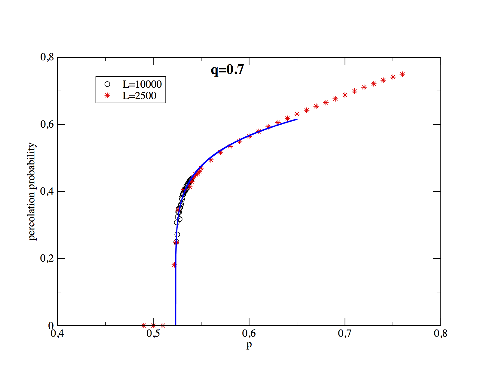
We show on Fig. 2 the numerical estimation of the percolation probability for , but we have also performed simulations for a wide range of values for which the percolation transition occurs. One finds near the threshold a scaling law . The value of the exponent is obtained by a power law fit. This requires a large lattice to avoid too large finite-size effects. For , we find , and for different values of , the results vary from 0.12 to 0.16. This is compatible, within error bars, with the exponent given by uncorrelated percolation, . We checked that a similar error bar range (containing the exact value) is obtained with an uncorrelated percolation model on a lattice of the same size. It is indeed well known [1] that very large lattice sizes are needed in order to accurately determine the critical exponents. Therefore, our results are consistent with a universal exponent for all values of .
3.1.3 Phase diagram
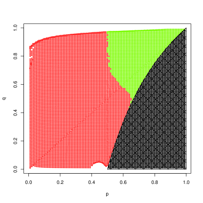
Fig. 3 represents the phase diagram of Hiebeler’s simulated habitats in the plane in terms of percolating or non-percolating phases. Because of the finite size of the configurations, the percolation threshold depends on the size of the lattice. It also varies from one configuration to another and it can be difficult to extrapolate with precision its (deterministic) value in an infinite lattice. However, we checked (see the colored/filled regions) that one can obtain stable results for the sizes studied, except in some regions of parameters (white/empty regions) where the Hiebeler algorithm is too slow to converge to the desired values.
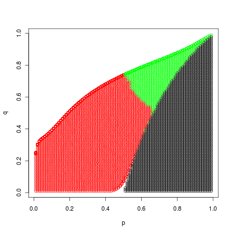
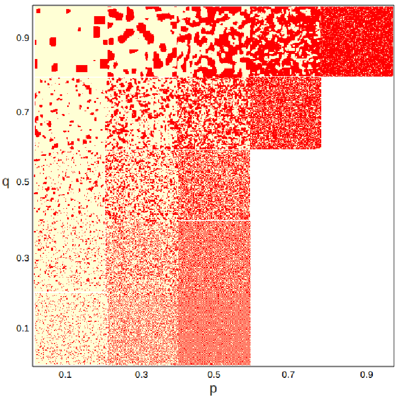
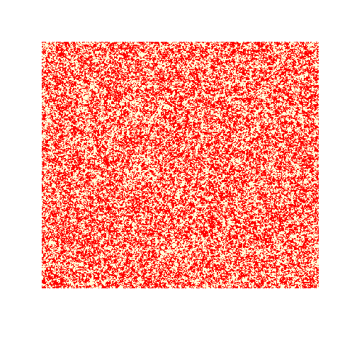
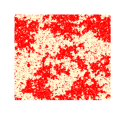
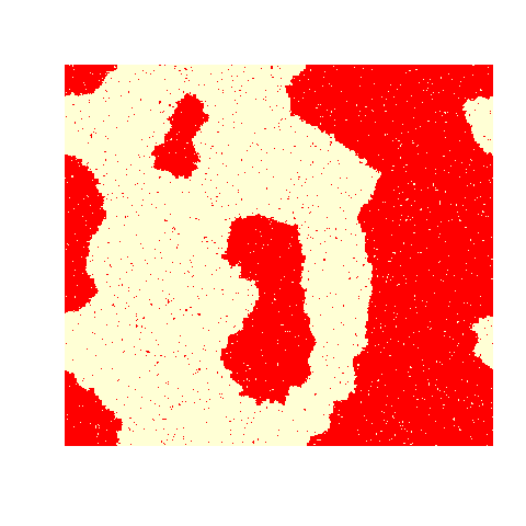
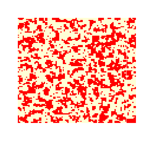
The transition line in the plane between the percolating phase and the non-percolating phase remains the same —up to convergence limitations— when one changes the algorithm generating the configurations. This is illustrated in Fig. 4 which corresponds to the modified algorithm where one proceeds by state permutations of neighboring sites. In this latter case, the convergence is slower than for Hiebeler’s algorithm, which is rather intuitive, considering that this other algorithm introduces space correlations (because of the choice of pairs of neighbors) compared to a single random choice of site. Typical configurations illustrating this percolating transition are presented in Fig. 5.
3.2 Cluster statistics and correlation functions
As in standard percolation theory, configurations of the above correlated percolation model -using Hiebeler’s algorithm- can be spatially characterized by cluster statistics and spatial correlation functions.
3.2.1 Size distribution of finite clusters
The size distribution of finite clusters (connected sets of suitable sites) is of great ecological relevance to characterize the patterns of insularity and fragmentation that constrain biodiversity dynamics. It recovers the general belief that not only habitat loss, but also habitat fragmentation and connectedness, matters to conservation issues [23].
Coniglio and collaborators [24, 25] presented percolation theory as the generic framework to investigate the distribution of clusters given the distribution of the constitutive elements (here suitable sites), with the underlying idea that geometrical clusters capture the physical properties of the substrate.
A relevant quantity is the distribution of clusters of suitable sites not belonging to the infinite cluster and belonging to a cluster of size . In the case of uncorrelated percolation, one has . A power-law behavior is observed only at the percolation transition, where the coherence length diverges according to the scaling law with , and [1].
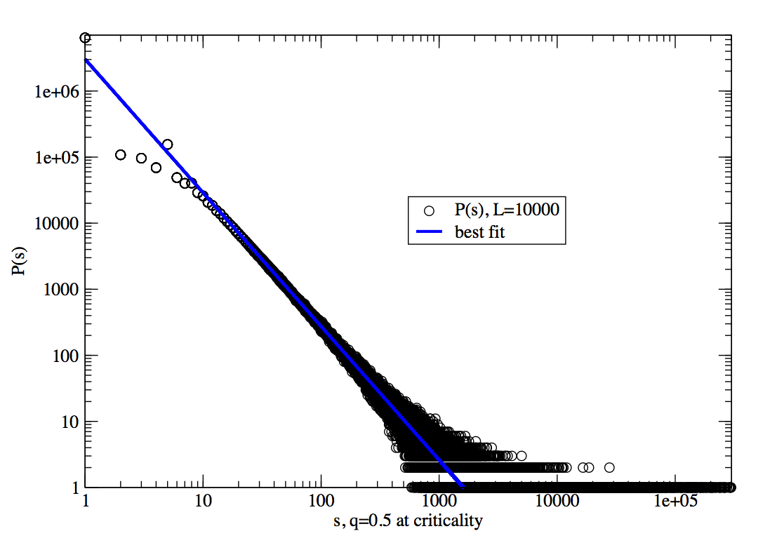
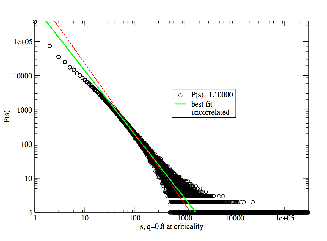
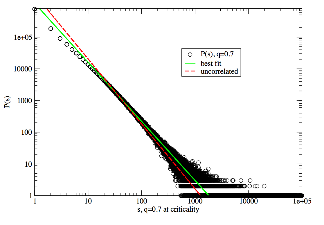
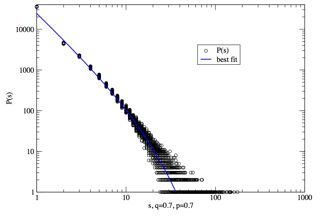
We calculated the cluster size distribution for the Hiebeler’s model at the critical point for various values of . At the percolation threshold, the distribution is a power-law , with an exponent which varies between 1.86 and 2.02 when varies. In all cases the value for uncorrelated percolation lies within the error bars obtained through the fitting procedure (Figs. 6 and 7). We checked that a similar error bar range (containing the exact value) is obtained with the uncorrelated percolation model at criticality () on a lattice of the same size.
Outside the threshold, is not a power law. It can be fitted by where the value of is again consistent with the uncorrelated percolation value. It is not our objective here to characterize precisely the critical behavior of , as it would require extensive simulation as a numerical project in itself. As far as the critical exponent is concerned, we can say that its value is compatible with the value of uncorrelated correlation.
In the case of correlated percolation, results available in the literature are scarce. A power-law decay is claimed to be found only at the transition [26]. Our results tend to confirm this property, together with the fact that critical exponents do not seem to change drastically between uncorrelated and correlated percolation.
3.2.2 Pair connectedness function
The pair connectedness function is defined as the probability that a site at distance from a suitable origin is suitable and belongs to the same finite cluster (the infinite cluster has to be removed from the computation) [25, 24]. Statistical isotropy of the model ensures that depends only on the modulus .
The typical behavior of this correlation function is
| (8) |
where defines another coherence length and characteristic cluster linear size (a priori different from ). For uncorrelated percolation, its has been shown [1] that which yields in (exponent values are rational in , according to conformal invariance arguments).
(i) At the percolation threshold For (uncorrelated percolation) we found = 0.1941, where the small discrepancy with the exact value can be attributed to finite-size effects. The values we found for correlated percolation deviate from the uncorrelated percolation value when increases: for the values of were respectively (Fig. 8). This trend would mean that seem to decrease more quickly as a function of the distance when the aggregation parameter is larger. The statistical analysis has been made using between 30 and 100 different configurations of a lattice of size . Even with such statistics, the results may not be completely converged. However, the discrepancy between the observed exponents and those of uncorrelated percolation still lies within the error bars and the range of finite-size fluctuations. It thus seems reasonable to state that Hiebeler’s model lies in the same universality class as uncorrelated percolation.
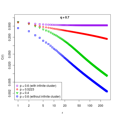
(ii) Outside the percolation threshold Considering only finite clusters, we studied the correlation function outside the percolated threshold and found a steeper decay of than at the threshold (Fig. 9), in agreement with equation (8), though it is not our purpose here to study systematically .
For non-percolating situations () this result is expected because the clusters are smaller than at the threshold. Above the threshold (), the decorrelation is steeper because only a few small isolated cluster remain apart from the dominant cluster (recall that is computed without taking into account the infinite cluster). Above the percolation threshold, when the dominant infinite cluster is considered in the calculation, converges to a value close to : the majority of sites belongs to the infinite cluster (Fig. 9). We compared the results found using different algorithms for generating the configurations (permutations of pairs of neighboring sites, or permutation of any pairs of sites) and found that the overall shape of is not affected.
3.2.3 Correlation function
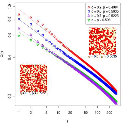
We have also calculated numerically the correlation function , defined as the probability that a site at a distance from a suitable site is also suitable, independently of the cluster it belongs to. Contrarily to which is a more local quantity, is more suitable to characterize the overall structure of the habitat. For = 1, we recover , the probability that a neighboring site of an suitable site is suitable. When increases, we observe a decorrelation and tends to .
Our numerical simulation shows that is always close to a power law (Fig. 11) with an exponent close to 1 at the percolation threshold, i.e. . Moreover we find no qualitative differences between percolating and non percolating situations: the exponent remains close to 1 when varying at a fixed value of , and even for different values of .
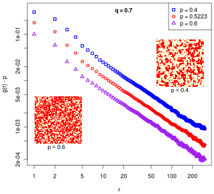
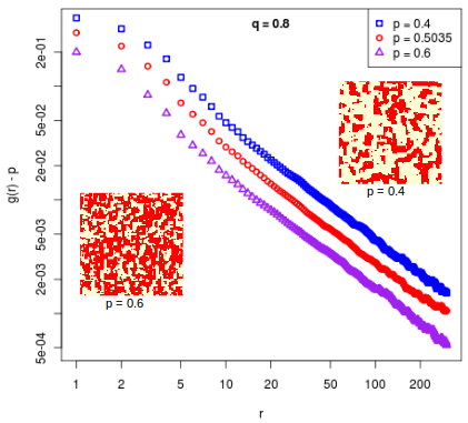
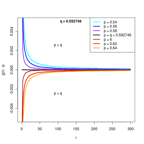
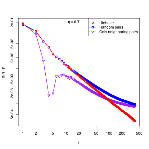
We checked the robustness of this result when one changes the algorithm used for habitat generation (Fig. 12). Strikingly, there are noticeable differences in (we checked, that for the quantity , the changes are minor). When one uses permutations of pairs of neighboring sites, decreases more slowly than a power law at large . At small distances, there exists a noticeable dip in the spatial correlations. Thus, the structure of the habitat is strongly changed at small and large distances. Hence Hiebeler’s original algorithm has its own special properties and cannot be considered as a universal scheme for correlated habitats.
4 Relation to the Ising model
The Hiebeler’s model locally prescribes correlation constraints. It is natural to compare this framework with the Ising’s model, which is the simplest model of short-range interactions in magnetism and a reference model in statistical physics [28, 29]. While nearest-neighbor pair correlations are prescribed in the Hiebeler’s model, they arise from the prescription of nearest-neighbor interactions (interaction parameter ) and the external magnetic field in the Ising’s model. However, even if the nearest-neighbor correlations of the two models coincide, long-range spatial order need not be the same in the two models. In particular, it has been shown that spatial correlations described by in the Ising’s model decrease exponentially fast [30] in marked contrast with the power-law behavior observed in the Hiebeler’s model. Moreover, starting from a given Ising’s model with parameters , one can derive the corresponding Hiebeler’s parameters . The correspondence is rather complex, since it may not be unique, especially in the case of symmetry breaking. This case occurs when one crosses the Ising critical point, at and : then a non-zero magnetization state and its opposite are equally equilibrium states (eq 9). Conversely, starting from the Hiebeler’s prescription, one can find corresponding Ising’s parameters only for a limited range of values.
The benefits of comparing the models is twofold. First, it allows to understand better the phases probed by Hiebeler’s prescriptions, in the light of what we know from the Ising’s phase diagram in the space. Secondly, it allows to probe other kinds of phases in the regions of the space that cannot be mapped onto an Ising’s model.
In the following, we will describe in detail all phases encountered in Hiebeler’s model in the cases where a clear correspondence with the Ising’s model is possible.
4.1 Ising model
The transformation maps the Boolean variables (with values and , used in the context of the Hiebeler’s model) to spin variables (with values or ).
Considering an Ising’s model with reduced [41] ferromagnetic interaction and reduced external field , it is described by the Hamiltonian:
| (9) |
where the second sum runs over the pairs of nearest neighbors. The global distribution (that is, the probability distribution in the space of the configurations on the lattice):
| (10) |
where is the partition function, ensuring a proper normalization of the distribution. The interaction can be either ferromagnetic () or antiferromagnetic .
4.2 Correspondence between Hiebeler’s and Ising’s model parameters
The calculation of and as a function of the Ising’s parameters can be an involved task. Consider for example the definition of : , where and are neighbors . One can write:
| (11) |
Hence comes from the following formula:
| (12) |
Because of non-vanishing terms in the Boltzmann factors involved in the calculation, we deduce that it is not possible at this stage to give an analytical correspondence between and except in the specific case for which .
In the case where , the Hamiltonian is reduced to: . Then, we have for any pair of nearest neighbors: and yielding explicit formulae for and .
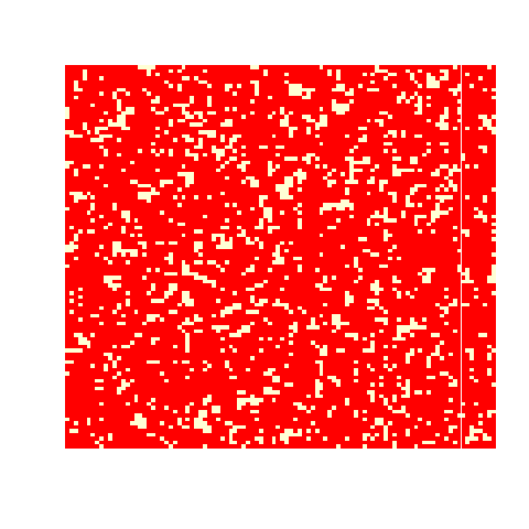
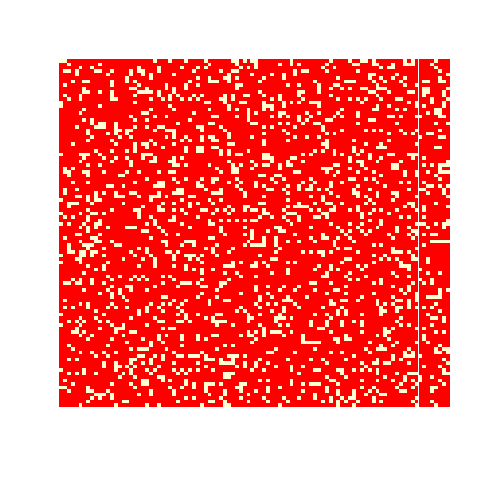
This absence of explicit link between and is due to the difference of constraint prescription in the two models. Starting from and , it is possible to find the corresponding and by numerical simulation, whereas the reverse is not true: the knwoledge of and is not enough to determine uniquely and . As an illustration, one can generate different configurations corresponding to the same values of obtained from two very different values of (Fig. 13).
4.3 Comparison of Hiebeler’s and Ising’s phases
We have simulated the Ising’s model for different values of using the Metropolis algorithm. After the convergence of the algorithm has been reached, we calculated the corresponding values of and (Figs. 14 and 15). Then we tried to relate the phases found for the Ising’s model to the phases studied previously in the plane.
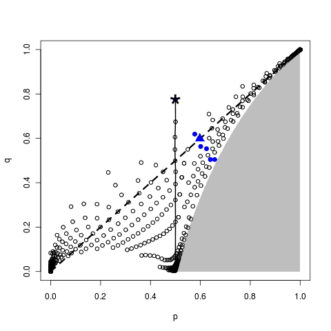
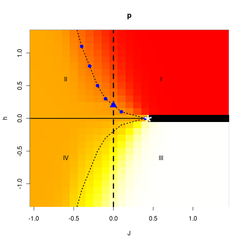
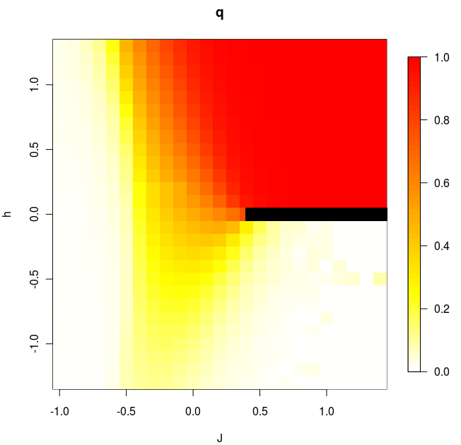
In Fig. 14 and Fig. 15 we represent the space of Hiebeler’s parameters explored by an Ising numerical simulation. We can see that for the (large) amplitude of and simulated, only a small part of the space of Hiebeler’s model parameters is explored (by comparing Fig. 14 and Fig. 5). We also show where the correlation percolation transition line in the plane can be found in the phase diagram for , but the Ising model does not describe the upper part of this percolation line (for and large). The in-depth presentation of the correspondence between the two models is provided in detail in the Appendix.
To conclude, we have seen that an Ising model is also an eligible model for correlated percolation, and that it contains part of the percolation phase diagram of the Hiebeler’s model. However, the Hiebeler’s model is richer in the sense that it generates other types of configurations. Moreover, the direct use of the density and aggregation parameter are somehow more intuitive in order to construct the desired types of habitat.
We underline that Ising’s model is thoroughly defined by the Hamiltonian , Eq. 9, which determines the global probability distribution , Eq. 10. In contrast, the knowledge of and alone does not determine the global probability distribution. It is straightforward to show that, in the domain where corresponds to a pair , the least biased distribution obtained by maximizing the Shannon entropy under the constraints given by and coincides with Ising’s distribution [31]. This remark indicates that additional prescriptions are contained in the Hiebeler’s algorithm which produce the observed phases and correlation structure. Indeed, the global spatial distribution is not only controlled by the parameters but also by the (non unique) way conditional probabilities at a larger distance and higher moments are related to and . A correspondence between the parameters is not enough to enforce an equivalence between Ising’s and Hiebeler’s models. In conclusion, we found that compared to Ising’s model, the Hiebeler’s algorithm richness lies in its diversity of types of generated configurations, both inducing longer-range correlations, and designing new configurations not contained in the Ising description.
5 Discussion
Ecologists often investigate the consequences of highly fragmented habitats in contrasted physical or land-use contexts for the maintenance of biodiversity [23]. Note that dynamical processes occurring on the habitat can change drastically the arrangement of suitable sites: in a dynamical model where the suitability of a site modifies back its suitability (mimicking the degradation of a suitable site due to grazing) [27], a power-law decay is observed for a wide range of values. Here, we limited ourselves to the case of a static habitat. We have investigated the properties of the Hiebeler model representing suitable and unsuitable habitat cells in a square lattice. This model is based on a density parameter, , and a parameter of short-range aggregation, . It is a special case of correlated percolation. The habitat parameterization is appealing for ecologists dealing with the short-range spatial dynamics of organisms in fragmented habitats, and as such it deserves in depth investigation of its spatial properties. We generated a diversity of habitat maps by varying the parameters , from fragmented to continuous, from random-like to highly clustered distributions. An important result is that the diversity of habitat configurations generated by the Hiebeler model is richer than the archetypal Ising model, which a statistical physicist would still choose naturally as a correlated percolation model (Figure 16). In fact, the Hiebeler’s model encompasses all the Ising phases, namely the antiferromagnetic, ferromagnetic and paramagnetic phases, as well as their transition points. However, we have showed that the space of configurations probed by the model can be different according to the algorithm implemented numerically. We thus underline that the parameterization does not provide unambiguous spatial properties, a fact that has been overlooked by ecologists and can strongly influence their models of organism dynamics in fragmented habitats. The parameters and are easy to estimate from experimental data. In ecology, habitat density and patch isolation are basic observable quantities that can be estimated from maps of environmental data. However the parameters should represent spatial contexts of habitats in a non ambiguous way, that is, they should fully prescribe the spatial properties. We have shown here that it requires additional information such as algorithmic constraints. This ambiguity, together with the speed of numerical convergence, are to be taken into account for further ecological studies. Furthermore, we have highlighted other quantities that should be measured by ecologists in order to get more insight on which model to rely on. Remarkably, the pair correlation function -in contrast to the pair-connectedness - can discriminate between different algorithm implementations of the Hiebeler model. Both quantities are hence of interest in ecology. Note that is intuitively useful in the framework of an underlying model with short-range dispersal, whereas is the natural quantity when one is interested by long-range dispersal.
The influence of correlations on the percolation universality class has been previously investigated in the literature, based on the large-distance behavior of . The exponent for the correlation length does not seem to change from its uncorrelated percolation value if the spatial correlations are short-range[9] [8] [32]. The model considered here with rather qualifies for long- range correlations. However, our results indicate that its critical properties do not markedly differ from those of the uncorrelated percolation. For all practical purposes, the universality class looks unaffected when non trivial nearest-neighbor conditional probabilities are prescribed (aggregation parameter ). Note that in the context of porous materials [3] the Hiebeler model (and is algorithmic variants) may correspond either to equilibrated materials or non-equilibrated materials (in the sense of having different synthesis protocols), all with the same prescriptions and . These would correspond to structures with the same critical exponents but different spatial correlations. This would certainly be of interest in future studies of porous materials.
From an ecologist point of view, the Hiebeler’s model can be a good one for simulating realistic habitats, as soon as one has evidence that the habitats to be modelled are indeed characterized by short-range aggregation. This can be checked for instance by measuring empirically and checking that it has an exponent not too far from the value for uncorrelated percolation. Then the aggregation parameter and the density can also be measured empirically and Hiebeler’s habitats can be simulated with these inputs, with an algorithm consistent with the measured . Even better, if one has a good knowledge of the processes underlying habitat formation, its topology, its ecological constraints, it will be easier to relate them to an instance of Hiebeler’s model. This opens the way for further studies of (i) the processes generating these habitats, (ii) the dynamics of organisms living and moving over the fragmented habitats. Although models of population dynamics over suitable localities (metapopulations) were first developed in a mean field perspective on a homogeneous substrate, following the seminal work of Levins [35, 36, 34], the colonization and extinction events depend in reality on the spatial distribution of suitable and unsuitable sites. The colonization process depends on the ability of individuals to move from a suitable occupied site to a suitable unoccupied one, is decreasing rapidly with distance, and therefore critically depends on habitat density and aggregation [38]. In particular, persistence will be related to the interplay between the spatial range of colonization and the aggregation parameter of the habitat. Our knowledge of the typical landscapes generated by the Hiebeler model will hence help us classify the outcome of metapopulation dynamics on such substrates.
6 Appendix
In this Appendix, we provide details on the correspondence between Hiebeler’s model and Ising’s model found in section IV. We refer in particular to Figures 14 and 15 in the main text.
The magnetization, defined for spin systems as , where the average is done over different realizations, is related to by: . We measured the magnetization as a function of for various values of (Fig. 16) and also as a function of for various values of (Fig. 17).
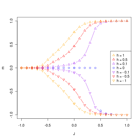
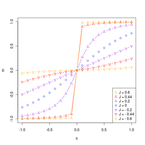
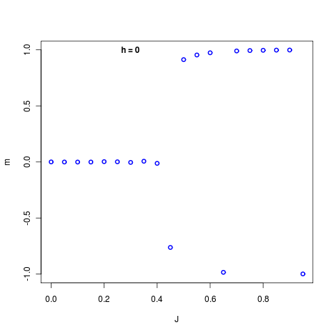
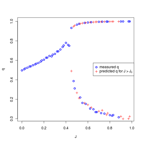
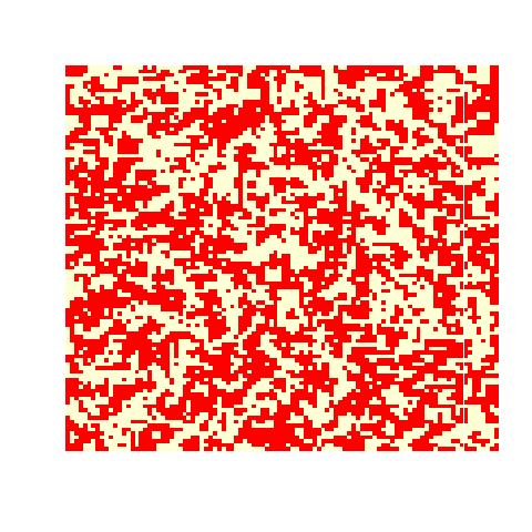
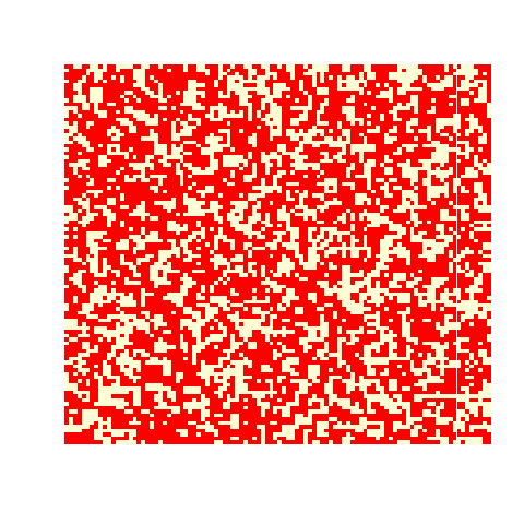
The usual phase transition of the Ising model can be recovered in this study. At zero field () and positive , there is a phase transition at . This is the well-known critical point of the Ising model, separating the paramagnetic phase () and the ferromagnetic phase (). Above the critical point one can illustrate the symmetry breaking as the density takes the value or at equilibrium depending on the initial configurations of the simulation. Similarly, two values of the conditional probability can be found: and (Fig. 18).
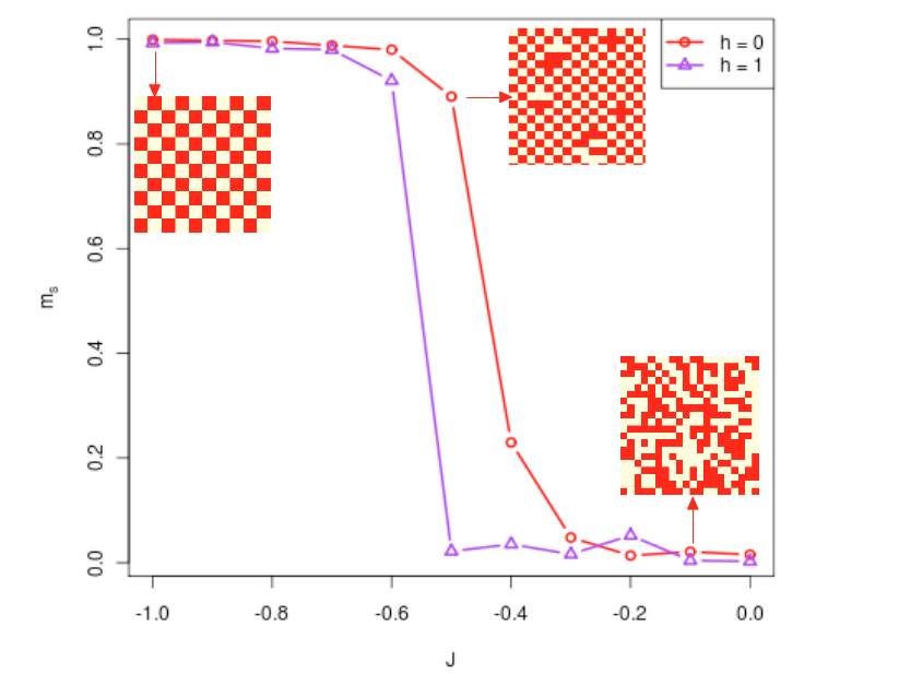
Let us now consider the case where and . It corresponds —in its larger part— to values of close to 1/2 and values of close to 0. It is also well-known that the Ising model undergoes a phase transition at , where the paramagnetic phase () is separated from the antiferromagnetic phase . The antiferromagnetic phase is characterized by a zero magnetization, since it corresponds to antiparallel configurations of spins. However one can characterize this phase by its non-vanishing staggered magnetization . A corresponds to a sub-lattice of lattice unit 2; B is the complementary sub-lattice of lattice unit 2. The antiferromagnetic transition is illustrated in Fig. 21 for two different values of .
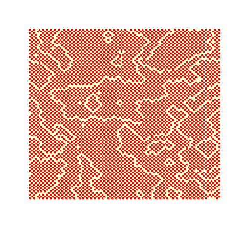
The antiferromagnetic phase can be found in particular in the Hiebeler’s phase diagram in a small region close to ; it is far from the percolating line, and requires a long time to reach equilibrium (for a typical realization, see Fig. 22).
We can now describe systematically the different types of configurations found by calculating the values of in the Ising plane .
In particular, the Ising critical point is on the percolation line of Hiebeler phase diagram. The other points on the percolation line correspond to : they correspond either to paramagnetic or antiferromagnetic phases.
-
1.
Line .
For , one has a ferromagnetic phase, and because there is a symmetry breaking: according to the initial configuration, simulation generates a mixture of such configurations. If , ; if , . If is larger but close to , in finite size, allowed values of and can take two possible values: and .
For there is a paramagnetic phase, with and .
For , and then decreases when decreases. For , and for , .
For there is an antiferromagnetic phase with . As decreases, tends to 0, tends to 1 and a perfectly alternate configuration with suitable and unsuitable sites is observed (Fig. 21).
-
2.
Line .
In this case there is an exact correspondence . This corresponds in Fig. 14 to the diagonal , namely uncorrelated percolation model. Percolation occurs at , which corresponds to a value such that . For there is percolation, for there is no percolation.
-
3.
Transition lines (dashed lines in Fig. 15) correspond either to a paramagnetic/ferromagnetic transition if or to a antiferromagnetic/ferromagnetic transition in non-zero field (cf magnetization and staggered magnetization profiles in Figs. 17 and 21). In fact the transition line in positive field coincide with the percolation line () of the correlated percolation model (blue dots, in both Fig. 14 and Fig. 15). However, one can have other points on the correlated percolation line (as seen in the Hiebeler’s phase diagram, for and ) where there is no possible correspondence with an Ising model. One has also particular points.
These remarkable points and lines allow to distinguish four different regions I, II, III and IV, that we describe here briefly.
-
1.
Region I: , , the symmetry breaking disappears because of the non-zero field; hence one tends to a ferromagnetic phase for with and . For however, one has an antiferromagnetic phase where is close to and varies between 1 and .
-
2.
Region II: , . If , one has a paramagnetic phase, with and close to . If one has an antiferromagnetic phase and .
-
3.
Region III: , , the symmetry breaking disappears because of the non-zero field; hence one tends to a ferromagnetic phase for with and . For however, one has an antiferromagnetic phase where is close to and varies between 0 and .
-
4.
Region IV: , . If , one has a paramagnetic phase, with and close to . If one has an antiferromagnetic phase and .
References
- [1] D. Stauffer and A. Aharony, Introduction to percolation theory (Taylor & Francis, London, 1994).
- [2] M. Laguës and A. Lesne, Scale Invariance, (Springer, Berlin, 2011), chap. 5.
- [3] A. Bejan and J. P. Zane, Design in Nature, Doubleday, New York, 2012. D. A. Nield and A. Bejan, Convection in Porous Media, 4th ed., Springer, 2013.
- [4] R. H. Gardner, B. T. Milne, M. G. Turner, and R. V. O’Neill, Landscape Ecology 1, 19 (1987)
- [5] R. V. O’Neill, R. H. Gardner and M. G. Turner, Landscape Ecology 7, 55 (1992).
- [6] G. P. Boswell, N. F. Britton, and N. R. Franks, Proc. Roy. Soc. B 265, 1921 (1998).
- [7] B. K. Chakrabarti, K. Kaski and J. Kertesz Phys.Lett. A 82, 97 (1981).
- [8] Z. Zhang, Phys. Lett. A 91, 246 (1982)
- [9] A. Weinrib, Phys. Rev. B 29, 387 (1984).
- [10] S. Prakash, S. Havlin, M. Schwartz, and H. E. Stanley, Phys. Rev. A 46, R1724 (1992).
- [11] H. E. Stanley, J. S. Andrade Jr., S. Havlin, H. A. Makse, and B. Suki, Physica A 266, 5 (1999).
- [12] T. Wiegand, K. Moloney, J. Naves and F. Knauer, Am. Nat. 154, 605 (1999).
- [13] D. Hiebeler, Ecology 81, 1629 (2000).
- [14] N. A. Thomson and S. P. Ellner, Theor. Pop. Biol. 64, 271 (2003).
- [15] D. Hiebeler, J. Math. Biol. 54, 337 (2007).
- [16] L. Russo, Z. Wahrscheinlichkeitstheorie verw. Gebiete 43, 39 (1978).
- [17] P. Bártfai and P. Revesz, Z. Wahrscheinlichkeitstheorie verw. Geb. 7, 43 (1967).
- [18] L. Sucheston, J. Math. Anal. Appl. 6, 447 (1963).
- [19] J. Hoshen and R. Kopelman, Phys. Rev. B 14, 3438 (1976).
- [20] J. W. Evans, J. Phys. A 20, 6487 (1987).
- [21] L. Turban, J. Phys. C. 12, 5009 (1979).
- [22] L. Turban and P. Guilmin, J. Phys. C. 12, 961 (1979).
- [23] L. Fahrig, Annu. Rev. Ecol. Evol. Syst. 34, 487 (2003).
- [24] A. Coniglio and L. Russo, J. Phys. A 12, 545 (1979).
- [25] A. Coniglio and A. Fierro, in Encyclopedia of Complexity and Systems Science, edited by R. A. Meyers (Springer, Berlin, 2008) pp. 1596–1615.
- [26] J. van den Berg, Ann. Appl. Prob. 21, 374 (2011).
- [27] S. Kéfi, M. Rietker, C. L. Alados, Y. Pueto, V. P. Papanastasis, A. ElAich, and P. C. de Ruiter, Nature 449, 213 (2007).
- [28] E. Ising, Z. Phys. 31, 253 (1925).
- [29] Baxter, Rodney J. (1982), Exactly solved models in statistical mechanics, London: Academic Press Inc.
- [30] J. W. Evans, D. R. Burgess and D. K. Hoffman, J. Math. Phys. 25, 3051 (1984).
- [31] C. Shannon, Bell System Tech. J. 27, 379 (1948)
- [32] C. M. Chaves and B. Koiller, Physica A 218, 271 (1995).
- [33] R. V. O’Neill, J. R. Krummel, R. H. Gardner, G. Sugihara, B. Jackson, D. L. DeAngelist, B. T. Milne, M. G. Turner, B. Zygmunt, S. W. Christensen, V. H. Dale, and R. L. Graham, Landscape Ecology 1, 153 (1998).
- [34] P. Amarasekare, Am. Nat. 152, 298 (1998).
- [35] R. Levins, Bull. Entomol. Soc. Am. 155, 237 (1969).
- [36] R. Lande, Am. Nat. 130, 624 (1987).
- [37] O. Ovaskainen and I. Hanski, Theor. Pop. Biol. 60, 281 (2001).
- [38] O. Ovaskainen, K. Sato, J. Bascompte, and I. Hanski, J. Theor. Biol. 215, 95 (2002).
- [39] J. Bascompte and R. V. Sole, J. Anim. Ecol. 65, 465 (1996).
- [40] F. Munoz, P. O. Cheptou, and F. Kjellberg, Ecol. Mod. 105, 314 (2007).
- [41] “Reduced” means that we group the temperature factor with the raw interaction strength into a dimensionless coupling constant .