The Idea and Concept of
Metos3D – A Marine Ecosystem Toolkit for Optimization and Simulation in 3-D
Abstract
The simulation and parameter optimization of coupled ocean circulation and ecosystem models in three space dimensions is one of the most challenging tasks in numerical climate research. Here we present a scientific toolkit that aims at supporting researchers by defining clear coupling interfaces, providing state-of-the-art numerical methods for simulation, parallelization and optimization while using only freely available and (to a great extend) platform-independent software. Besides defining a user-friendly coupling interface (API) for marine ecosystem or biogeochemical models, we heavily rely on the Portable, Extensible Toolkit for Scientific computation (PETSc) developed in Argonne Nat. Lab. [1] for a wide variety of parallel linear and non-linear solvers and optimizers. We specifically focus on the usage of matrix-free Newton-Krylov methods for the fast computation of steady periodic solutions, and make use of the Transport Matrix Method (TMM) introduced by Khatiwala et al. in [8].
Key words: Coupled tracer simulation, Optimization, Marine ecosystem models, Biogeochemical models, Matrix-free inexact Newton-Krylov, Coupling interface
1 Introduction
Here we describe the main features of coupled ocean circulation and ecosystem models and how Metos3D will help to flexibly perform simulation and optimization runs for a wide range of model configurations.
1.1 Coupled Ocean Circulation and Ecosystem Models and Simulations
Marine ecosystem models play an important role for the investigation of the global carbon cycle. The ocean water takes up a huge amount of from the atmosphere, and the question how long the carbon (or carbon dioxide) remains in the ocean – especially in the deeper layers – clearly effects the future uptake and thus also prognoses on climate change. Coupled ocean circulation and ecosystem models consist of two parts, namely the ocean circulation itself and the biogeochemistry describing (or trying to describe) the interplay between marine chemistry, marine biology and the geological conditions and processes. The main coupling direction between both parts (at least the one that in many cases is considered only) is the one from ocean circulation to biogeochemistry, whereas the inverse coupling is less clear and often ignored in coupled models and simulations. When running biogeochemistry model with given ocean circulation without taking into account this inverse effect, sometimes the notions offline computation or (for the simulated quantities) passive tracers is used.
Whereas for the ocean circulation the governing equations are quite clear (Navier-Stokes equations, temperature/energy equation, and transport equation for salinity), for biogeochemical models there is a big variety. The models can have from two up to dozen of tracer variables, and consequently a similar different number of transport equations. Moreover, many model parameters (as growth or dying rates) are not directly measurable. Therefore there is a high demand on parameter optimization to obtain those that fit the model output to given observational data, and furthermore a need for a possibility to quickly examine changes within parameters, parameterizations or even number of tracers and model structure. Preferably this should be done within a three dimensional physics, on a global scale and using circulation from an up-to-date ocean circulation or global climate model.
When performing a coupled simulation, both parts (i.e. the simulation of the ocean circulation and of a biogeochemical model) usually require a huge amount of computing time, especially in three space dimensions. In a typical case, a coupled run from a spatially constant tracer distribution to a steady periodic solution takes thousands of years of model time.
1.2 Idea and Structure of Metos3D
The idea of Metos3D is to provide a toolkit that has the following properties:
-
•
It allows a flexible coupling of the ocean model component and the biogeochemistry part for simulation. In the first place it provides a coupling to a transport matrix method introduced by Khatiwala et al., see [8].
-
•
It provides an interface/API between a quite general class of marine biogeochemical models that can be coupled to the ocean model part and to the simulation and optimization methods. It offers the opportunity to use tools of Algorithmic/Automatic Differentiation (AD, see e.g. [6]) for simulation, sensitivity computations and optimization.
-
•
It provides a Newton-based method to compute steady periodic solutions as well as a classical pseudo time-stepping spin-up. It deploys state-of-the-art techniques of scientific computing including equation solvers, optimization routines and parallelization techniques to accelerate all simulation and optimization runs. Here Metos3D is based on the well-established PETSc library, see [1].
-
•
It relies only on software which is freely and public available and runs on different platforms.
-
•
The implementation is platform-independent and allows coupling of models written in C and Fortran.
2 Marine Ecosystem Tracer Simulation
Marine biogeochemical tracers are substances in the ocean water that are undergoing chemical or biochemical reactions. The processes in this ecosystem are thus governed by time dependent transport equations with additional, usual non-linear coupling terms. Since the ocean circulation determines the tracer transport, solving these equations means solving the Navier-Stokes equations to obtain the turbulent mixing/diffusion coefficients and the velocity field for advection.
2.1 Transport Equations
The system of transport equations for the vector of tracers generally reads
| (1) |
where is the velocity vector and the turbulent mixing/diffusion coefficient. Both have to satisfy the Navier-Stokes equations which can be solved simultaneously with (1) or (in the so-called offline mode) in advance.
The usual non-linear coupling term (also called source minus sink or SMS term) models the interaction between the tracers, e.g. photosynthesis and growth and dying or consumption processes. Their modeling involve several only heuristically determined parameters, here summarized in a vector , that are often the subject of parameter optimization in order to fit the model to given data.
2.2 Marine Ecosystem Models
There is a wide range of marine biogeochemical or ecosystem models. They vary in the number of tracers and thus equations, and moreover in the number and types of processes they model and the way how they do this. In these parametrizations the model parameter vector plays an important role: The number and meaning of the parameters differ from model to model. To handle a wide range of ecosystem models thus requires a high flexibility in the number of both tracers and parameters.
Examples for tracers are nitrate, phosphate, chlorofluorocarbons or carbon dioxide. Modeling the carbon cycle for example requires describing alkalinity, a complex reaction of inorganic tracers. A detailed description of this reaction can be found in the online document about the design of OCMIP-2 simulations (Ocean Carbon-Cycle Model Intercomparison Project, http://www.ipsl.jussieu.fr/OCMIP/phase2/simulations/design.ps).
Phosphate on the other hand is a major nutrient for ocean biota (organisms) which is represented by organic tracers in biogeochemical models, either implicitly by dissolved organic phosphorus, nitrogen or carbon or explicitly by phytoplankton or zooplankton. Thus in this case the intent of the model equations is to describe processes like nutrient consumption, growing, grazing or dying rather than chemical reactions.
Most models also admit terms representing sinking of inorganic tracers, like iron or calcite particles, and organic tracers, like detritus (dead matter) or particulate organic phosphorus. Moreover all these processes depend on many external geographic conditions, i.e. precipitation, insolation, air pressure or latitude.
In the following we will describe two simple global models based on inorganic phosphate (, or for short) as an example.
2.2.1 Example 1: The PO4-DOP Model
The PO4-DOP model admits phosphate and dissolved organic phosphorus (DOP). The tracers are denoted by . The biological production (the net community productivity) is calculated as a function of nutrients and light . The production is limited using a half saturation function, also known as Michaelis-Menten kinetics, and a maximum production rate parameter .
Light, here, is a portion of short wave radiation , which is computed as a function of latitude and season following the astronomical formula of Paltridge and Platt [12]. The portion depends on the photo-synthetically available radiation , the ice cover and the exponential attenuation of water.
A fraction of the biological production remains suspended in the water column as dissolved organic phosphorus, which remineralizes with a rate . The remainder of the production sinks as particulate to depth where it is remineralized according to the empirical power law relationship determined by Martin et al. [11]. Similar descriptions for biological production can be found in [13], [4] and [14].
Moreover the model formulation consists of a production (sun lit, euphotic) zone, with a depth of , and a noneuphotic zone, and respectively. The equations read
| in | ||||
| in | ||||
| in | ||||
| in , |
where
The following table summarizes the parameters within the PO4-DOP model:
| Symbol | Description | Unit |
|---|---|---|
| maximum community production rate | ||
| attenuation of water | ||
| half saturation constant of PO4 | ||
| half saturation constant of light | ||
| remineralization rate of DOP | ||
| fraction of DOP, | ||
| sinking velocity exponent |
2.2.2 Example 2: The PO4-DOP-PHY Model
The PO4-DOP-PHY model admits explicitly modeled phytoplankton (PHY), which is implicitly prescribed within the parameter in the former model for example. The tracers are denoted by .
The biological production additionally depends now on the phytoplankton concentration and a growth rate
while the computation of light do not change. The fraction of phytoplankton that is grazed is controlled by . Additionally there are three loss rates and for phytoplankton. They can be considered as parameterization of various processes like mortality rate, aggregation of cells and immediate sinking or viral infections. Their detailed description can be found in Kriest et al [10]. The model equations read
where
Again, the following table summarizes the model parameters:
| Symbol | Description | Unit |
|---|---|---|
| maximum growth rate of PO4 | ||
| attenuation of water | ||
| half saturation constant of PO4 | ||
| half saturation constant of insolation | ||
| remineralization rate of DOP | ||
| fraction of DOP, | ||
| loss rate of PHY, euphotic zone | ||
| quadratic loss rate of PHY, euphotic zone | ||
| loss rate of PHY, whole water column | ||
| grazing fraction, | ||
| sinking velocity exponent |
3 Transport Matrix Approach
In the first place we provide the pre-computed ocean circulation fields by so-called transport matrices. In [8] Khatiwala et al. presented an approach well suited for passive tracer simulation. Their method is a good trade-off between complexity and accuracy. Moreover the assumption they make, i.e. important biogeochemical processes happen within a water column (and a small zone around it), matches ours for the biogeochemical interface (see Section 5.1).
The idea is based on the linearity of the time dependent diffusion and advection operators. The system of transport equations can always be written as
where admits both, diffusion and advection, and becomes a block diagonal matrix after discretization. Due to the locality of the differential operators the matrices remain extremely sparse for large systems of equations. Using basis functions, can be evaluated and stored.
In doing so several aspects have to be taken into account. The choice of appropriate basis functions is crucial to avoid too sharp gradients or too high diffusivity. Moreover modern ocean circulation models consist of operator splitting schemes to tackle the different spacial extents of the ocean. Operators effecting the longitudinal and latitudinal directions are treated explicitly, while vertical effects are computed implicitly in time. This results in two different types of matrices.
A compromise has to be found for storage too. Here Khatiwala et al. propose monthly averaged diffusion and advection matrices, which can be interpolated during computation. Their experiments show that twelve explicit and twelve implicit matrices provide a sufficient accuracy at minimal storage requirements.
Nevertheless, using a transport matrix approach, the whole coupled simulation results in a scheme of matrix-vector multiplications and evaluations of the biogeochemical model. Hence
Its simplicity is clearly an advantage compared to other couplings. There is still a resolved seasonal cycle and a sparse matrix-vector multiplication is a well supported standard operation in numerical libraries. Moreover no diffusion and advection have to be implemented.
4 Spin Up and Computation of Periodic Solutions
Transport equations – after spatial discretization – can be viewed as a subclass of systems of ordinary differential equations. They are in most cases solved by a time-integration procedure, i.e. an Euler or Runge-Kutta type method. Given a coupling term the solution depends on the so called forcing, i.e. the turbulent mixing/diffusion coefficient, the velocity vector, wind, insolation etc., which can be time dependent. These data are either given or can be (pre-)computed by an ocean circulation model. In biogeosciences it is common to search for solutions forced by climatological (time dependent but periodic) data. Here the notion dynamical spin up problem or (for the solution) equilibrium is used.
For a given time interval the process of integration over the whole interval from an initial value defines a mapping with
while for the solution the periodic property reads
Thus a periodic solution is a fixed point for the – in general nonlinear – mapping .
5 Biogeochemical Model Interface
As indicated in the former sections marine ecosystem simulations are complex at all points. On the one hand they are computationally costly, on the other hand they admit a large variety of biogeochemical models. Especially the latter highlights a need for the possibility of quickly examine new model formulations and parameterizations. Consequently our intent is to propose an interface for coupling ocean physics to biogeochemical models.
5.1 Assumptions and Description
The main assumption we make is that, regarding biogeochemistry, the most important processes happen within a water column, even in three space dimensions. This assumption is not definitive and can change in the future, but seems to be reasonable in the beginning. It simplifies the implementation of a model a lot and, as we will see, does not constrain the interface too much. Thus the interface admits, besides the number of layers and tracers, and respectively, an array of given tracer concentrations for a water column and an array for computed tracer concentrations by the model .
The second assumption made is that the year consists of 360 days. This becomes of importance when regarding the ocean time step and the point in time . Moreover it has an effect on the provided, precomputed short wave radiation .
Considering light computations from the latter, see Section 2.2.1, the interface additionally provides the fraction of day , the ice cover as well as the heights and depths for the current water column.
Another important aspect in biogeochemical models is the air-sea gas transfer. It depends on the mentioned ice cover and the wind speed on the surface. Moreover the latitude of the water column, the water temperature and salinity are needed for its computation.
Last by not least the interface provides a possibility to pass parameters to the model. Their number is denoted by and the array by .
The following table summarizes the input and output arguments of the interface, their notations, ranges, units and short descriptions.
| Notation | Range | Unit | Description |
|---|---|---|---|
| - | point in time | ||
| - | ocean time step | ||
| ∘ | latitude | ||
| short wave radiation | |||
| - | fraction of day | ||
| - | ice cover | ||
| wind speed | |||
| - | number of tracers | ||
| - | number of layers | ||
| array of layer heights | |||
| array of layer depths | |||
| array of salinity | |||
| array of temperature | |||
| array of tracer concentrations | |||
| computed source/sink array | |||
| - | number of parameters | ||
| - | array of parameters |
5.2 Realization in C and FORTRAN
In C real numbers are realized as double and natural numbers as int. An array is represented by a pointer and its length is either the according int argument (one-dimensional array) or the product of several corresponding int arguments (multidimensional array). Hence
void bgc(
double t, double dt,
double lat, double insol, double dayfrac, double ice, double wind,
int ntracer, int nlayer,
double *h, double *d, double *salt, double *temp,
double *y, double *ybgc,
int nparam, double *u
);
In FORTRAN real numbers are realized as real*8 and natural numbers as integer. An arrays is denoted as a variable with one or more dimensions (ranks). Its length is either its dimension (one-dimensional array) or the product of dimensions (multidimensional array). Hence
subroutine bgc(
t, dt, lat, insol, dayfrac, ice, wind,
ntracer, nlayer,
h, d, salt, temp, y, ybgc,
nparam, u
)
real*8 :: t, dt, lat, insol, dayfrac, ice, wind
integer :: ntracer, nlayer
real*8 :: h(nlayer), d(nlayer), salt(nlayer), temp(nlayer)
real*8 :: y(nlayer, ntracer), ybgc(nlayer, ntracer)
integer :: nparam
real*8 :: u(nparam)
6 PETSc Solvers
The PETSc library offers several variants of sophisticated nonlinear equation solvers. Its two basic techniques are a globalized Newton method using a cubic interpolation as line search (LS) method and an adaption of the Trust Region Method for nonlinear equations. Detailed descriptions on both can be found in optimization textbooks, e.g. in [3]. Both approaches require solving a linear system of equations with the Jacobian of the nonlinear mapping introduced in Section 4.
6.1 Matrix-Free Linear System Solvers
In many systems resulting from three-dimensional spatial discretizations of PDEs, the Jacobian is too big to even store it, specifically if it is dense. A remedy is to use matrix-free iterative Krylov subspace methods as Conjugate Gradients or GMRES, which are also supplied by PETSc.
The Jacobian-vector product needed in a single Newton (and also Trust Region) step can be approximated by finite differences, or alternatively be computed exactly using Automatic Differentiation.
6.2 Inexact Computation and Compatibility of Stopping Criteria
The linear system of equations is always solved with a prescribed accuracy, but tight tolerances for inexact residuals can lead to ”oversolving”. Eisenstat and Walker described in [5] the fundamentals for inexact (truncated) Newton methods, namely the way how to adjust inner (i.e. linear system solver) and outer (i.e. Newton or Trust Region iteration) stopping tolerances. This methodology is also already implemented in the PETSc library.
7 First Exemplary Results
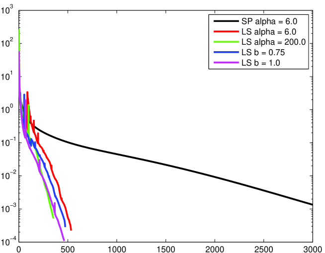
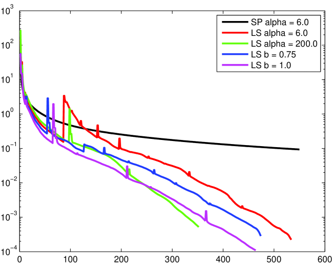
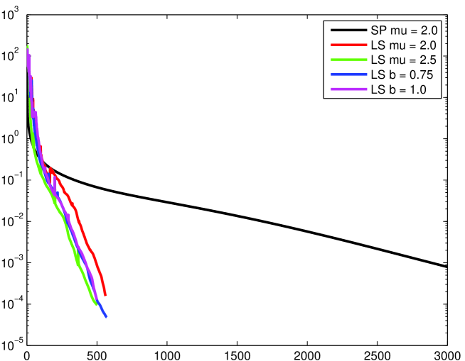
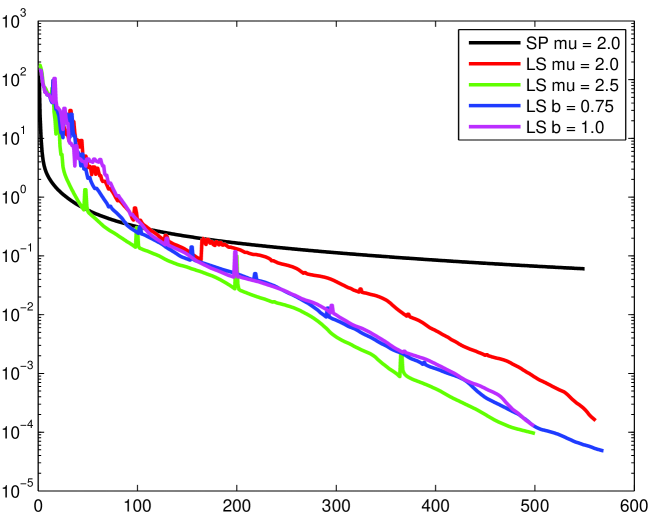
In the following we present different convergence results for the PO4-DOP and PO4-DOP-PHY model. The computations were performed on a Linux cluster with 2.1 GHz AMD Barcelona CPUs. They show the behavior of a globalized Newton-Krylov solver provided by the PETSc library in contrast to a usual spin-up, which can be interpreted as a fixed point iteration.
The ocean circulation is computed using twelve implicit and twelve explicit matrices, which are linearly interpolated over 2880 time steps, corresponding to one year. They represent monthly averaged diffusion and advection and were evaluated using the MIT general circulation model (http://mitgcm.org/) with a latitudinal and longitudinal resolution of and 15 vertical layers. This resolution results in a vector length of 52749 per tracer. More details on the configuration of ocean physics can be found in [8].
The biogeochemical models consist of two euphotic layers and eight internal time steps per one ocean step. They were implemented in FORTRAN and coupled to the ocean circulation using the described interface.
The solution we are looking for is a fixed point for the mapping that integrates the tracers forward in time for one year. The figures show the the Euclidean norm of the difference between the concentrations before and after the integration
where is the vector of all tracers.
The error of the spin-up, i.e. the fixed point iteration, is computed after every year of integration. The convergence results of the nonlinear solver depict the error of the residual after every Newton step and the error of the Krylov solver in between. The former uses a line search technique with cubic backtracking. The latter is a GMRES solver with a finite differences approximation for the Jacobian vector product, a restart parameter of 200 and a modified Gram-Schmidt orthogonalization. The tolerances for the Krylov subspace solver are chosen depending on the residual norm after each Newton step, see [5]. Except restart and orthogonalization standard PETSc settings are used.
8 Flexibility and Portability
Our entitlement is to provide a software that is as flexible and portable as possible. Concerning the biogeochemical models we presented an interface which is a first step towards this requirement.
Regarding the hardware there is demand for flexibility and portability too. On the one hand it should be possible to make low resolution test runs on the home PC with a multi core processor. On the other hand high resolution parameter optimization clearly requires massively parallel hardware. Thus Metos3D is based on PETSc.
First of all the library is open-source and freely available. It has been developed for 15 years now and is well maintained. Moreover there are over 200 applications, extensively tested on different platforms, using PETSc.
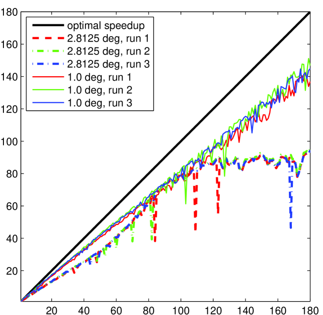
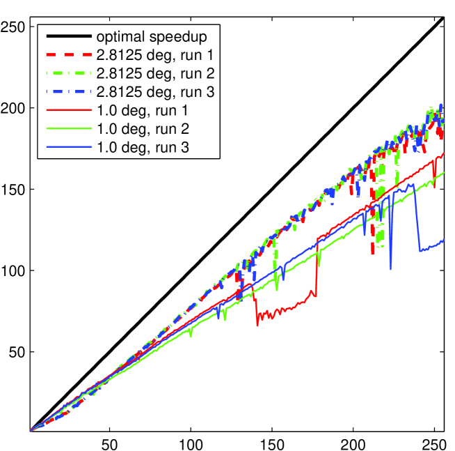
The following figures show speedup test runs on different parallel hardware. One is a Linux cluster (rzcluster) with 192 AMD Barcelona processors located at the University of Kiel. The other is a massively parallel hardware ( 20000 processors) located in Hannover and Berlin. It is part of the North-German Supercomputing Alliance (HLRN, http://www.hlrn.de/).
The tests were performed with a and a resolution to investigate the impact of the different load distributions on the speedup.
9 Next Steps
As already pointed out in the title, this preprint is a first conceptual overview of the desired structure and features of Metos3D. We here additionallly list some keywords that indicate the future direction of our work:
-
•
Krylov subspace methods unfold their whole potential with a preconditioner, compare [9], which is up to now not realized.
-
•
Moreover we can easily integrate an interface for AD processed models/source code.
References
- [1] Satish Balay, Kris Buschelman, William D. Gropp, Dinesh Kaushik, Matthew G. Knepley, Lois Curfman McInnes, Barry F. Smith, and Hong Zhang. PETSc Web page, 2009. http://www.mcs.anl.gov/petsc.
- [2] Peter N. Brown and Youcef Saad. Hybrid krylov methods for nonlinear systems of equations. SIAM J. Sci. Stat. Comput., 11:450–481, May 1990.
- [3] J.E. Dennis and R.B. Schnabel. Numerical methods for unconstrained optimization and nonlinear equations. Society for Industrial Mathematics, 1996.
- [4] S. Dutkiewicz, M. Follows, and P. Parekh. Interactions of the iron and phosphorus cycles: A three-dimensional model study. Global Biogeochem. Cycles, 19:1–22, 2005.
- [5] Stanley C. Eisenstat and Homer F. Walker. Choosing the forcing terms in an inexact newton method. SIAM Journal on Scientific Computing, 17(1):16–32, 1996.
- [6] A. Griewank and A. Walther. Evaluating derivatives: principles and techniques of algorithmic differentiation. Society for Industrial and Applied Mathematics (SIAM), 2008.
- [7] Thomas Kaminski, Ralf Giering, and Michael Voßbeck. Efficient sensitivities for the spin-up phase. In H. M. Bücker, G. Corliss, P. Hovland, U. Naumann, and B. Norris, editors, Automatic Differentiation: Applications, Theory, and Implementations, Lecture Notes in Computational Science and Engineering, pages 285–293. Springer, 2005.
- [8] S. Khatiwala, M. Visbeck, and M.A. Cane. Accelerated simulation of passive tracers in ocean circulation models. Ocean Modelling, 9(1):51–69, 2005.
- [9] Samar Khatiwala. Fast spin up of ocean biogeochemical models using matrix-free newton-krylov. Ocean Modelling, 23(3-4):121 – 129, 2008.
- [10] I. Kriest, S. Khatiwala, and A. Oschlies. Towards an assessment of simple global marine biogeochemical models of different complexity. Progress In Oceanography, 86(3-4):337 – 360, 2010.
- [11] J.H. Martin, G.A. Knauer, D.M. Karl, and W.W. Broenkow. Vertex: carbon cycling in the northeast pacific. Deep Sea Research Part A. Oceanographic Research Papers, 34(2):267–285, 1987.
- [12] G. W. Paltridge and C. M. R. Platt. Radiative processes in meteorology and climatology, 318 pp, 1976.
- [13] P. Parekh, M.J. Follows, and E.A. Boyle. Decoupling iron and phosphate in the global ocean. Global Biogeochemical Cycles, 19, 2005.
- [14] Y. Yamanaka and E. Tajika. Role of dissolved organic matter in the marine biogeochemical cycle: Studies using an ocean biogeochemical general circulation model. Global Biogeochemical Cycles, 11(4):599–612, 1997.