Towards a Compiler for Reals

Abstract

Numerical software, common in scientific computing or embedded systems, inevitably uses an approximation of the real arithmetic in which most algorithms are designed. In many domains, roundoff errors are not the only source of inaccuracy and measurement and other input errors further increase the uncertainty of the computed results. Adequate tools are needed to help users select suitable approximations, especially for safety-critical applications.

We present the source-to-source compiler Rosa which takes as input a real-valued program with error specifications and synthesizes code over an appropriate floating-point or fixed-point data type. The main challenge of such a compiler is a fully automated, sound and yet accurate enough numerical error estimation. We present a unified technique for floating-point and fixed-point arithmetic of various precisions which can handle nonlinear arithmetic, determine closed- form symbolic invariants for unbounded loops and quantify the effects of discontinuities on numerical errors. We evaluate Rosa on a number of benchmarks from scientific computing and embedded systems and, comparing it to state-of-the-art in automated error estimation, show it presents an interesting trade-off between accuracy and performance.

1 Introduction

Numerical software, common in scientific computing and embedded systems, inevitably approximates the real arithmetic in which its algorithms are typically designed. In addition to roundoff errors from finite-precision arithmetics such as floating-point or fixed-point, many problem domains come with additional sources of imprecision, such as measurement and truncation errors, increasing the uncertainty on the computed results. We need adequate tools to help developers understand whether the computed values meet the accuracy requirements and remain meaningful in the presence of the errors. This is particularly important for safety-critical systems.

Today, however, accuracy in numerical computations is often an afterthought. We write programs in a user-selected finite-precision data type and then, perhaps, try to verify that it meets our expectations. This is problematic for several reasons. Firstly, it introduces a mismatch between the real-valued algorithms we write on paper and the low-level implementation details of floating-point or fixed-point arithmetic. Secondly, finite-precision source code semantics prevents the compiler from applying many optimizations (soundly), as, for instance, associativity no longer holds. And lastly, numerical errors remain implicit if they are only the result of some separate analysis tool.

We propose a different strategy. The programmer writes the program in a real-valued specification language and makes numerical errors explicit in pre- and postconditions. It is then up to our compiler to determine an appropriate data type which fulfills the specification but is as efficient as possible and to generate the corresponding code. This is in particular attractive for fixed-point arithmetic, often used in embedded systems, where the code generation can be quite challenging as the programmer has to ensure (implicit) decimal points are aligned correctly.

Clearly, one of the key challenges of such a compiler is to determine how close a finite-precision representation is to its ideal implementation in real numbers. While techniques exist which can handle linear operations successfully [Goubault and Putot (2011), Darulova and Kuncak (2011)], precise and sound error estimation remains difficult in the presence of nonlinear arithmetic. Roundoff errors and error propagation depend on the ranges of variables in complex and non-obvious ways; even determining these ranges precisely for nonlinear code poses a challenge. Furthermore, due to numerical errors, the control flow in the finite-precision implementation may diverge from the ideal real-valued one, taking a different branch and producing a result that is far off the expected one. Quantifying discontinuity errors is hard due to many correlations and nonlinearity but also due to lack of smoothness or continuity of the underlying functions that arise in practice [Chaudhuri et al. (2011)]. In loops, roundoff errors grow, in general, unboundedly. Even if an iteration bound is known, loop unrolling approaches scale poorly when applied to nonlinear code.

We have addressed these challenges and present here our results towards the goal of a verifying compiler for real arithmetic. In particular, we present

• a real-valued implementation and specification language for numerical programs with uncertainties; we define its semantics in terms of verification constraints that they induce.

• an approximation procedure for computing precise range bounds for nonlinear expressions which combines SMT solving with interval arithmetic.

• an approach for sound and fully automatic error estimation for nonlinear expressions for floating-point as well as fixed-point arithmetic of various precisions. We handle roundoff and propagation errors separately with affine arithmetic and a first-order Taylor approximation, respectively. While providing accuracy, this separation also allows us to provide the programmer with useful information about the numerical stability of the computation.

• an extension of the error estimation to programs with simple loops, where we developed a technique to express the total error as a function of the number of loop iterations.

• a sound and scalable technique to estimate discontinuity errors which crucially relies on the use of a nonlinear SMT solver.

• an open-source implementation in a tool called Rosa which we evaluate on a number of benchmarks from the scientific computing and embedded systems domain and compare to state-of-the-art tools.

2 A Compiler for Reals

We first introduce Rosa’s specification language and give a high-level overview of the technical challenges and our solutions on a number of examples.

A Real-Valued Specification Language Rosa is a ‘verifying’ source-to-source compiler which takes as input a program written in a real-valued non-executable specification language and outputs appropriate finite-precision code. A program is written in a functional subset of the Scala programming language and consists of a number of methods over the Real data type. Figures 1,4 and 5 show three such example methods. Pre- and postconditions allow the user to explicitly state possible errors on method inputs and maximum tolerable errors on the output(s), respectively. Taking into account all uncertainties and their propagation, Rosa chooses a data type from a range of floating-point and fixed-point precisions and emits the corresponding implementation in the Scala programming language.

By writing programs in a real-valued source language, programmers can reason about the correctness of the real-valued algorithm, and leave the low-level implementation details to the automated sound analysis in Rosa. Besides this separation of concerns, the real-valued semantics also serves as an unambiguous ideal baseline against which to compute errors. We believe that making numerical errors explicit in pre- and postcondition attached directly to the source code makes it less likely that these will be forgotten or overlooked. Finally, such a language opens the door to sound compiler optimizations exploiting properties which are valid over reals, but not necessarily over finite-precision - as long as the accuracy specification is satisfied.

Compilation Algorithm If a full specification (pre- and postcondition) is present on a method, Rosa analyzes the numerical computation and selects a suitable finite-precision data type which fulfills this specification and synthesizes the corresponding code. The user can specify which data types are acceptable from a range of floating-point and fixed-point precisions. The order in which these possible data types are given is important. Rosa searches through the data types, applying a static analysis for each, and tries to find the first in the list which satisfies the specification. While this analysis is currently repeated for each data type, parts of the computation can be shared and we plan to optimize the compilation process in the future.

The selection and the order of data types may depend on resource limits. If, for example, a floating-point unit is not available or would be very costly, the programmer can prioritize fixed-point data types. In general, the larger the data type (in terms of bits) the more time and memory the execution will take. We illustrate the performance vs. accuracy trade-off for the sine function from Figure 1 in the graph in Figure 2, which shows the runtime and accuracy and in particular the trade-off between the two for different data types. Rosa helps programmers navigate this trade-off space by providing automated sound accuracy estimates.

Rosa can also be used as an analysis tool. By providing one data type (without necessarily a postcondition), Rosa will perform the analysis and report the results, consisting of a real-valued range and maximum error of the result, to the user. These analysis result are also reported during the regular compilation process as they may yield useful insights.

⬇

def sineWithError(x: Real): Real = {

require(x > -1.57079632679 && x < 1.57079632679 && x +/- 1e-11)

x - (x*x*x)/6.0 + (x*x*x*x*x)/120.0 - (x*x*x*x*x*x*x)/5040.0

} ensuring(res => res +/- 1.001e-11)

Figure 1: Approximation of sine with a Taylor expansion

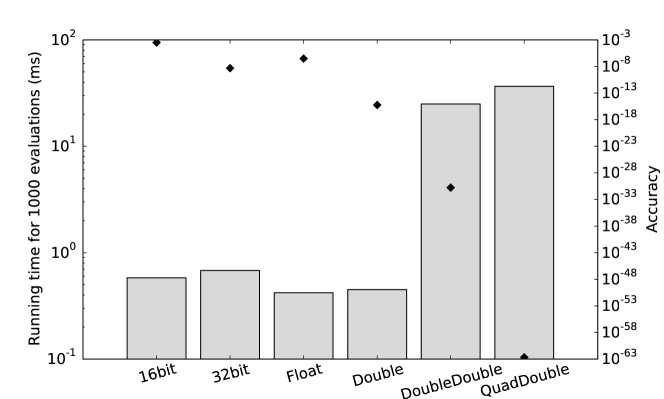
Figure 2: Running times vs accuracy for different finite-precision data types

⬇

/*

@param x (x +/- 1.e-11)

@return ((-1.0003675439019308 <= result && result <= 1.0003675439019308 &&

(result +/- 3.8907801077969955e-09)))

*/

def sineWithError(x : Long): Long = {

require(-1.5707963268 <= x && x <= 1.5707963268)

val _tmp1 = ((x * x) >> 31)

val _tmp2 = ((_tmp1 * x) >> 30)

val _tmp3 = ((_tmp2 << 30) / 1610612736l)

val _tmp4 = ((x << 1) - _tmp3)

val _tmp5 = ((x * x) >> 31)

val _tmp6 = ((_tmp5 * x) >> 30)

val _tmp7 = ((_tmp6 * x) >> 31)

val _tmp8 = ((_tmp7 * x) >> 31)

val _tmp9 = ((_tmp8 << 28) / 2013265920l)

val _tmp10 = ((_tmp4 + _tmp9) >> 1)

val _tmp11 = ((x * x) >> 31)

val _tmp12 = ((_tmp11 * x) >> 30)

val _tmp13 = ((_tmp12 * x) >> 31)

val _tmp14 = ((_tmp13 * x) >> 31)

val _tmp15 = ((_tmp14 * x) >> 30)

val _tmp16 = ((_tmp15 * x) >> 31)

val _tmp17 = ((_tmp16 << 23) / 1321205760l)

val _tmp18 = (((_tmp10 << 1) - _tmp17) >> 1)

val result = _tmp18

}

Figure 3: Sine function implemented in fixed-point arithmetic

2.1 Example 1: Straight-line Nonlinear Computations

We illustrate this compilation process on the example in Figure 1, which shows the code of a method which computes the sine function with a 7th order Taylor approximation. The Real data type denotes an ideal real-valued variable without uncertainty or roundoff. The require clause specifies the range of the input parameter x as well as an initial uncertainty of 1e-11, which may stem from previous computations or measurement imprecisions. We would like to make sure that error on the result does not grow too large, so we constrain the error to 1.001e-11. We leave the data type unconstrained, so that Rosa considers 8, 16 and 32bit fixed-point arithmetic as well as single, double, double double and quad double floating-point precision by default (in this order). Rosa determines that 8 bit fixed-point precision potentially overflows, 16 or 32 bit fixed-point arithmetic is not accurate enough (total error of 2.54e-4 and 3.90e-9 respectively) and that single-precision floating-point arithmetic is neither (error of 2.49e-7). For double floating-point precision, Rosa determines the error of 1.000047e-11, so that it generates code over the Double data type. If we could accept a somewhat larger error, say 5e-9, then Rosa determines that 32bit fixed-point arithmetic is sufficient. We show the generated code in Figure 3. (All intermediate results fit into 32 bits, but as we need up to 64 bits to perform the arithmetic operations, we simulate the arithmetic here with the 64 bit Long data type.) Note that the generated code retains part of the precondition. In Scala, require expressions are actually runtime checks that throw an exception if the given condition is violated. Our error analysis, and code generation as well, is only valid if the range and error of the input is satisfied. We can only check the ranges at runtime, and Rosa generates the constraints such that they check the actual range (i.e. the ideal real-valued ranges $\pm$ all possible errors). Checking the result range with a postcondition is not necessary, since Rosa has already proven those bounds correct.

In order to determine which data type is appropriate, Rosa performs a static analysis which computes a sound estimate of the worst-case absolute error. Since roundoff errors and error propagation depend on the ranges of (all intermediate) computations, Rosa needs to compute these as accurately as possible. We developed a technique which combines interval arithmetic [Moore (1966)] with a nonlinear SMT solver, which provides accuracy as well as automation (section 4). In addition, using an SMT solver allows Rosa to take into account arbitrary additional constraints on the inputs, which, for example, neither interval nor affine arithmetic [de Figueiredo and Stolfi (2004)] can. Rosa decomposes the total error into roundoff errors and propagated initial errors and computes each differently (section 5). The accumulation of roundoff errors is kept track off with affine arithmetic, while propagation errors are soundly estimated with a first-order Taylor approximation. The latter is fully automatically and accurately computed with again the help of a nonlinear SMT solver.

2.2 Example 2: Loops with Constant Ranges

⬇

def sine(x: Real): Real = {

require(-20 <= x && x <= 20)

x - x*x*x/6 + x*x*x*x*x/120

}

def pendulum(t: Real, w: Real, n: LoopCounter): (Real, Real) = {

require(-2 <= t && t <= 2 && -5 <= w && w <= 5 &&

-2.01 <= ~t && ~t <= 2.01 && -5.01 <= ~w && ~w <= 5.01)

if (n < 100) {

val h: Real = 0.01

val L: Real = 2.0

val m: Real = 1.5

val g: Real = 9.80665

val k1t = w

val k1w = -g/L * sine(t)

val k2t = w + h/2*k1w

val k2w = -g/L * sine(t + h/2*k1t)

val tNew = t + h*k2t

val wNew = w + h*k2w

pendulum5(tNew, wNew, n++)

} else {

(t, w)

}

}

Figure 4: Simulation of a pendulum

In general, numerical errors in loops grow unboundedly and the state-of-the-art to compute sound error bounds in complex code is by unrolling. It turns out, however, that our separation of errors into roundoff and propagation errors allows us to express the error as a function of the number of loop iterations. We have identified a class of loops for which we can derive a closed-form expression of the loop error bounds. This expression, on one hand, constitutes an inductive invariant, and, on the other hand, can be used to compute concrete error bounds. While this approach is limited to loops where the variable ranges are bounded, our experiments show that this approach can already analyze interesting loops that are out of reach for current tools.

Figure 4 shows such an example: a Runge Kutta order 2 simulation of a pendulum. t and w are the angle the pendulum forms with the vertical and the angular velocity respectively. We approximate the sine function with its order 5 Taylor series polynomial. We focus on roundoff errors between the system following the real-valued dynamics and the system following the same dynamics but implemented in finite precision (we do not attempt to capture truncation errors due to the numerical integration, nor due to the Taylor approximation of sine). After 100 iterations, for instance, Rosa determines that the error on the results is at most 8.82e-14 and 1.97e-13 (for t and w respectively) when implemented in double-precision floating-point arithmetic and 7.38e-7 and 1.65e-6 in 32 bit fixed-point arithmetic.

2.3 Example 3: Discontinuities

⬇

def jetApproxGoodFitWithError(x: Real, y: Real): Real = {

require(-5<=x && x<=5 && -5<=y && y<=5 && x +/- 0.001 && y +/- 0.001)

if (y < x) {

-0.317581 + 0.0563331*x + 0.0966019*x*x + 0.0132828*y +

0.0372319*x*y + 0.00204579*y*y

} else {

-0.330458 + 0.0478931*x + 0.154893*x*x + 0.0185116*y -

0.0153842*x*y - 0.00204579*y*y

}

}

Figure 5: Approximation of a complex embedded controller

Embedded systems often use piece-wise approximations of more complex functions. In Figure 5 we show a possible piece-wise polynomial approximation of a fairly complex jet engine controller. We obtained this approximation by fitting a polynomial to a sample of values of the original function. Note that the resulting function is not continuous.

A precise constraint encoding the difference between the real-valued and finite-precision computation, if they take different paths, features variables that are tightly correlated. This makes it hard for SMT-solvers to cope with and makes linear approaches imprecise. We explore the separation of errors idea in this scenario as well, to soundly estimate errors due to conditional branches. We separate the real-valued difference from finite-precision artifacts. The individual error components are easier to handle individually, yet preserve enough accuracy.

In our example, the real-valued difference between the two branches is bounded by 0.0428 (making it arguably a reasonable approximation given the large possible range of the result). However, this is not a sound estimate for the discontinuity error in the presence of roundoff and initial errors (in our example 0.001). With Rosa, we can confirm that the discontinuity error is bounded by 0.0450 with double floating-point precision, with all errors taken into account.

3 Problem Definition

Clearly, error computation is the main technical challenge of our compiler for Reals. Before we describe our solution in detail, we first precisely define the error computation problem that Rosa is solving internally. Formally, an input program consists of one or more methods given by the grammar in Figure 6.

⬇

P $::=$ def mName(args): res = {

require(A₁ $\land$ $\ldots$ $\land$ A_n)

( L | D | B )

}

A $::=$ C | $x$ +/- const | S

S $::=$ S $\land$ S | S $\lor$ S | $\neg$ S | C

L $::=$ if (n < const) mName(B, n + 1) else args

D $::=$ if (C) D else D | B

B $::=$ val $x$ = F; B | F

F $::=$ F + F | F - F | F * F | F / F | $\sqrt{\text{F}}$ | X

C $::=$ F $\leq$ F | F < F | F $\geq$ F | F > F

X $::=$ $x$ | const

Figure 6: Rosa’s input language

args denotes possibly multiple arguments and res can be a tuple. The method body may consist of the standard arithmetic operators ${+,-,*,/,\sqrt{}}$, as well as immutable variable declarations (val t1 = ...), functional calls and conditionals. Note that square root is only supported for floating-point arithmetic. The specification language is functional, so we represent loops as recursive functions (denoted L), where n denotes the integer loop iteration counter. For loop-free code D, note that more complex conditions on branches can be expressed with nesting.

Let us denote by $P$ a real-valued function representing our program and by $x$ its input. Denote by $\tilde{P}$ the corresponding finite-precision implementation of the program, which has the same syntax tree but with operations interpreted in finite-precision arithmetic. Let $\tilde{x}$ denote the input to this finite-precision program. The technical challenge of Rosa is to estimate the difference:

$$\max_{x,\tilde{x}}\;\;\lvert P(x)-\tilde{P}(\tilde{x})\rvert$$ (1)

which denotes the absolute error of the result of the program. This error is crucial for selecting an implementation data type.

The domains of $x$ and $\tilde{x}$, over which this expression is to be evaluated, are given by the user-provided precondition in the require clause. It defines range bounds $x_{i}\in[a_{i},b_{i}],\tilde{x}_{i}\in[c_{i},d_{i}]$ for each component of the possibly multivariate input, as well as absolute error bounds on the inputs of the form $x_{i}\;$ +/- $\;\lambda_{i}$ that define the relationship $\lvert x-\tilde{x}\rvert\leq\lambda$, understood component-wise. If no errors are given explicitly, we assume roundoff as the initial error. The ability to specify initial errors in addition to roundoff is important for modular verification where the errors of one method may feed to following ones. Additionally, the require clause may specify further constraints on the inputs, such as x*x + y*y <=20.0. Method calls are handled either by inlining the postcondition or the whole method body.

Corresponding to the syntactic program is a real-valued mathematical expression which is the input to our core error computation procedure. Concretely, the input consists of one or several real-valued functions $f:\mathbb{R}^{m}\to\mathbb{R}^{n}$ over some inputs $x_{i}\in\mathbb{R}$, representing the arithmetic expressions F. We denote by $f$ and $x$ the exact ideal real-valued function and variables and by $\tilde{f}:\mathbb{R}^{m}\to\mathbb{R}^{n},\tilde{x}_{i}\in\mathbb{R}$ their actual finite-precision counter-parts. Note that for our analysis all variables are real-valued; the finite-precision variable $\tilde{x}$ is considered as a noisy versions of $x$. We perform the error computation with respect to some fixed target precision in floating-point or fixed-point arithmetic; this choice gives error bounds for each individual arithmetic operation.

When $P$ consists of a nonlinear arithmetic expression alone (F), then Equation 1 reduces to bounding the absolute error on the result of evaluating $f(x)$ in finite precision arithmetic: $\max_{x,\tilde{x}}\lvert f(x)-\tilde{f}(\tilde{x})\rvert$ (section 5). When the body of $P$ is a loop (L), then the constraint reduces to computing the overall error after $k$-fold iteration $f^{k}$ of $f$, where $f$ corresponds to the loop body. We define for any function $H$: $H^{0}(x)=x$, $H^{k+1}(x)=H(H^{k}(x))$. We are then interested in bounding (section 6):

$$\max_{x,\tilde{x}}\lvert f^{k}(x)-\tilde{f}^{k}(\tilde{x})\rvert$$

For code containing branches (grammar rule D), Equation 1 accounts also for the discontinuity error. For example, if we let $f_{1}$ and $f_{2}$ be the real-valued functions corresponding to the if and the else branch respectively with the if condition $c$, then, if $c(x)\land\lnot c(\tilde{x})$, the discontinuity error is given by $\lvert f_{1}(x)-\tilde{f}_{2}(\tilde{x})\rvert$, i.e., it accounts for the case where the real computation takes the if-branch, and the finite-precision one takes the else branch. The overall error on $P$ from Equation 1 in this case must account for the maximum of discontinuity errors between all pairs of paths, as well as propagation and roundoff errors for each path (section 7).

A note on relative error Our technique soundly overestimates the absolute error of the computation. A sound estimate of the relative error can be computed from this and from the range of the result provided that the range does not include zero. Whenever this is the case, Rosa also reports the relative error in addition to the absolute one.

3.1 Finite-precision Arithmetic

Rosa supports analysis and code generation for floating-point and fixed-point arithmetic of different precisions. We assume IEEE754 floating-point semantics. We regard overflow and underflow as errors and Rosa will report the possibility of these occurring as such. We assume rounding to nearest, however as long as the roundoff error can be determined from the range of possible values, our analysis can be straight-forwardly adapted. Code generation currently supports standard single and double floating-point arithmetic, as well as double-double and quad-double precisions implemented in software [Bailey et al. (2013)].

Fixed-point arithmetic also represents a subset of the rationals, but unlike floating-point arithmetic does not require specialized hardware. Instead, it is implemented with integer operations only, which makes it attractive especially for resource-bound systems. The consequence of this is, however, that the alignment of (implicit) decimal points has to be performed manually with bit shift operations at compile time. For this, the global ranges at each intermediate computation step have to be known, respectively have to be computed. For more details please see Anta2010, whose fixed-point semantics we follow.

While the input and output language is a subset of Scala, the analysis is programming language agnostic, providing the IEEE 754 standard is supported, and adapting Rosa to a different back-end would be straight-forward.

4 Computing Ranges Accurately

The first step to accurately estimating roundoff and propagation errors is to have a procedure to estimate ranges as tightly as possible. This is important as these errors directly depend on the ranges of all, including intermediate, values and coarse range estimates may result in inaccurate errors computed or make the analysis impossible due to spurious potential runtime errors (division by zero, etc.).

4.1 Interval and Affine Arithmetic

Traditionally, guaranteed computations have been performed with interval arithmetic [Moore (1966)]. Interval arithmetic computes a bounding interval for each basic operation as

$$x\circ y=[min(x\circ y),max(x\circ y)]\quad\quad\circ\in\{+,-,*,/\}$$

and analogously for square root. For longer computations, interval arithmetic introduces over-approximations, as it cannot track correlations between variables (e.g. $x-x\neq 0$).

Affine arithmetic [de Figueiredo and Stolfi (2004)] partially addresses this loss of correlation by representing possible values of variables as affine forms

$$\hat{x}=x_{0}+\sum_{i=1}^{n}x_{i}\epsilon_{i}$$

where $x_{0}$ denotes the central value (of the represented interval) and each noise symbol $\epsilon_{i}$ is a formal variable denoting a deviation from this central value, intended to range over $[-1,1]$. The maximum magnitude of each noise term is given by the corresponding $x_{i}$. The range represented by an affine form is computed as

$$[\hat{x}]=[x_{0}-rad(\hat{x}),x_{0}+rad(\hat{x})],\quad\quad rad(\hat{x})=\sum_{i=1}^{n}|x_{i}|$$

Note that the sign of the $x_{i}$s does not matter in isolation, it does, however, reflect the relative dependence between values. E.g., take $x=x_{0}+x_{1}\epsilon_{1}$, then

$$x-x =x_{0}+x_{1}\epsilon_{1}-(x_{0}+x_{1}\epsilon_{1})=x_{0}-x_{0}+x_{1}\epsilon_{1}-x_{1}\epsilon_{1}=0$$

If we subtracted $x^{\prime}=x_{0}-x_{1}\epsilon_{1}$ instead, the resulting interval would have width $2*x_{1}$ and not zero. Linear operations are performed term wise and are computed exactly, whereas nonlinear ones need to be approximated. Affine arithmetic can thus track linear correlations, it is, however, not generally better than interval arithmetic: e.g. $x*y$, where $x=[-5,3],y=[-3,1]$ gives $[-13,15]$ in affine arithmetic and $[-9,15]$ in interval arithmetic.

4.2 Range Estimation using Satisfiability Modulo Theories (SMT) Solvers

⬇

def getRange(expr, precondition, precision, maxIterations):

z3.assertConstraint(precondition)

[aInit, bInit] = evalInterval(expr, precondition.ranges);

//lower bound

if z3.checkSat(expr < a + precision) == UNSAT

a = aInit

b = bInit

numIterations = 0

while (b-a) < precision $\wedge$ numIterations < maxIterations

mid = a + (b - a) / 2

numIterations++

z3.checkSat(expr < mid) match

case SAT $\Rightarrow$ b = mid

case UNSAT $\Rightarrow$ a = mid

case Unknown $\Rightarrow$ break

aNew = a

else

aNew = aInit

//upper bound symmetrically

bNew = ...

return: [aNew, bNew]

Figure 7: Algorithm for computing the range of an expression

While interval and affine arithmetic are reasonably fast for range estimation, they tend to introduce over-approximations, especially if the input intervals are not sufficiently small. We improve over them by combining interval arithmetic with a nonlinear SMT (Satisfiability Modulo Theories) constraint solver to obtain automation and accuracy.

Figure 7 shows the algorithm for computing the lower bound of a range. The computation for the upper bound is symmetric. For each range to be computed, our technique first computes an initial sound estimate of the range with interval arithmetic. It then performs an initial quick check to test whether the computed first approximation bounds are already tight. If not, it uses the first approximation as the starting point and then narrows down the lower and upper bounds using a binary search. At each step of the binary search our tool uses the nonlinear nlsat solver within Z3 [De Moura and Bjørner (2008), Jovanović and de Moura (2012)] to confirm or reject the newly proposed bound. The search stops when either Z3 fails, i.e. returns unknown for a query or cannot answer within a given timeout, the difference between subsequent bounds is smaller than a precision threshold, or the maximum number of iterations is reached. This stopping criterion can be adjusted by the user.

Additional Constraints In our approach, since we are using Z3 to check the soundness of bounds, we can assert the additional constraints and perform all checks with respect to all additional and initial constraints. This is especially useful when taking into account branch conditions from conditionals.

Optimizations Calling an SMT solver is fairly expensive so we want to minimize the number of calls. The algorithm Figure 7 presents several direct knobs to do this: the maximum number of iterations and the precision of the range estimate. Through our experiments we have identified suitable default values, which seem to present a good trade-off between accuracy and performance. In addition to these two parameters, if we are only interested in the final range, we do not need to call Z3 and the algorithm in Figure 7 for every intermediate expression. In principle, we could call Z3 only on the full expression, however, we found that this resulted in suboptimal results as this expression very often was too complex. We found a good compromise in calling Z3 only every 10 arithmetic operations. All of these parameters can be adjusted by the user.

5 Soundly Estimating Numerical Errors in Nonlinear Expressions

Now we address the first challenge of error estimation for a loop-free nonlinear function without branches: $\lvert f(x)-\tilde{f}(\tilde{x})\rvert\text{ where }\lvert x-\tilde{x}\rvert\leq\lambda,f:\mathbb{R}^{m}\to\mathbb{R}^{n}$ and where the ranges for $x$ and $\tilde{x}$ are given by the precondition.

5.1 Error Estimation with Affine Arithmetic

Consider first roundoff errors only that is, we are interested in $\lvert f(x)-\tilde{f}(x)\rvert$, where the input errors are zero. Our procedure executes the computation abstractly by computing an interval and an affine form for each AST node:

⬇

(range: Interval, $\hat{err}$: AffineForm)

range represents the real-valued range, and $\hat{err}$ the accumulated worst-case errors, with essentially one noise term for each roundoff error (together with artifacts from nonlinear approximations). The actual finite-precision range is then given by range + $[\hat{err}]$, where $[\hat{err}]$ denotes the interval represented by the affine form. For each computation step, we compute the

1. new range with our range procedure from section 4

2. propagation of already accumulated errors

3. new roundoff error, which is then added to the propagated affine form.

Since we compute the range at each intermediate node, we also check for possible overflows, underflows, division by zero or negative square root errors without extra effort.

Propagation of Errors with Affine Arithmetic For linear operations, errors are propagated with the standard rules of affine arithmetic. For multiplication, division and square root the error propagation depends on the range of values, so that we have to adapt our computation to use the ranges computed with our Z3-backed procedure. In the following, we denote the real range of a variable $x$ by $[x]$ and its associated error by the affine form $\hat{err_{x}}$. When we write $[x]*\hat{err}_{y}$ we mean that the interval $[x]$ is converted into an affine form and the multiplication is performed in affine arithmetic. Multiplication is computed as

$$x*y =([x]+\hat{err_{x}})([y]+\hat{err_{y}})$$

$$=[x]*[y]+[x]*\hat{err_{y}}+[y]*\hat{err_{x}}+\hat{err_{x}}*\hat{err_{y}}+\rho$$

where $\rho$ is the new roundoff error. Thus the first term contributes to the ideal range and the remaining three to the error affine form. The larger the factors $[x]$ and $[y]$ are, the larger the finally computed errors will be so that a tight range estimation is important for accuracy. Division is computed as

$$\frac{x}{y} =x*\frac{1}{y}=([x]+\hat{err_{x}})([1/y]+\hat{err_{1/y}})$$

$$=[x]*[\frac{1}{y}]+[x]*\hat{err_{\frac{1}{y}}}+[\frac{1}{y}]*\hat{err_{x}}+\hat{err_{x}}*\hat{err_{\frac{1}{y}}}+\rho$$

For square root, we first compute an affine approximation of square root as in our previous work [Darulova and Kuncak (2011)]:

$$\sqrt{x}=\alpha*x+\zeta+\theta$$

and then perform the affine multiplication term wise.

Roundoff Error Computation Roundoff errors for floating-point arithmetic are computed at each computation step as

⬇

$\rho$ = $\delta$ * maxAbs(totalRange)

where $\delta$ is the machine epsilon, and added to $\hat{err}$ as a fresh noise term. Note that this roundoff error computation makes our error computation parametric in the floating-point precision. Since we regard (and report) subnormal numbers as errors, this error abstraction is sound. For fixed-point arithmetic, roundoff errors are computed as

⬇

$\rho$ = getFormat(totalRange, bitWidth).quantizationError

where the getFormat function returns the best fixed-point format [Anta et al. (2010)] that can accommodate the range. This computation is parametric in the bit-width.

5.2 Separation of Errors

We could use the affine arithmetic based procedure to track all errors,not only roundoff errors, by simply adding the initial error as a fresh noise term at the beginning. Such an approach treats all errors equally: the initial errors are propagated in the same way as roundoff errors which are committed during the computation. We found, however, that the over-approximation introduced by affine arithmetic for nonlinear computations increases substantially as the magnitude of the noise terms (i.e. the errors) becomes larger. Instead, we separate the total error as follows:

$$\textstyle\begin{split}\lvert f(x)-\tilde{f}(\tilde{x})\rvert&=\lvert f(x)-f(\tilde{x})+f(\tilde{x})-\tilde{f}(\tilde{x})\rvert\\ &\leq\lvert f(x)-f(\tilde{x})\rvert+\lvert f(\tilde{x})-\tilde{f}(\tilde{x})\rvert\end{split}$$ (2)

The first term, $\lvert f(x)-f(\tilde{x})\rvert$, captures the error on the result of $f$ caused by the initial error between $x$ and $\tilde{x}$. The second term, $\lvert f(\tilde{x})-\tilde{f}(\tilde{x})\rvert$, covers the roundoff error committed when evaluating $f$ in finite precision, but note that we can now compute this roundoff error on the same input $\tilde{x}$. Thus, we separate the overall error into the propagation of existing errors, and the newly committed roundoff errors. We denote by $\sigma_{f}:\mathbb{R}^{m}\to\mathbb{R}^{n}$ the function which returns the roundoff error committed when evaluating an expression $f$ in finite-precision arithmetic: $\sigma_{f}(\tilde{x})=\lvert f(\tilde{x})-\tilde{f}(\tilde{x})\rvert$. We omit the subscript _f, when it is clear from the context. Further, $g:\mathbb{R}^{m}\to\mathbb{R}^{n}$ denotes a function which bounds the difference in $f$, given a difference in its inputs: $\lvert f(x)-f(y)\rvert\leq g(\lvert x-y\rvert)$. When $m,n>1$, the absolute values are component-wise, e.g. $g(\lvert x_{1}-y_{1}\rvert,\dots,\lvert x_{m}-y_{m}\rvert)$, but when it is clear from the context, we will write $g(\lvert x-y\rvert)$ for clarity. Thus, the overall numerical error is given by:

$$\lvert f(x)-\tilde{f}(\tilde{x})\rvert\leq g(\lvert x-\tilde{x}\rvert)+\sigma(\tilde{x})$$ (3)

One alternative to Equation 2 would be to bound the error by $\lvert f(x)-\tilde{f}(x)\rvert$ $+\lvert\tilde{f}(x)-\tilde{f}(\tilde{x})\rvert$. The first term now corresponds to roundoff errors, but the second requires bounding the difference of $\tilde{f}$ over a certain input interval. In the separation that we have chosen, we need to compute the difference over the real-valued $f$. Note that $f$ is a simpler function than its finite-precision counterpart, and its analysis is reusable across different concrete implementations.

The function $\sigma$ is instantiated with the affine arithmetic based procedure from subsection 5.1. Since roundoff errors are local, we found affine arithmetic suitable for this purpose. In contrast, the propagation of existing errors (function $g$) depends highly on the steepness of the function, so we want to capture as much global information, such as correlations between variables, as possible. This is only feasible when looking at the function as a whole.

5.3 Propagation Errors

We instantiate Equation 3 with $g(x)=K\cdot x$, i.e. $\lvert f(x)-f(y)\rvert\leq K\lvert x-y\rvert$ which bounds the deviation on the result due to a difference in the input by a linear function in the input errors. The constant $K$ (or vector of constants $K_{i}$ in the case of a multivariate function) is to be determined for each function $f$ individually, and is usually called the Lipschitz constant. We will also use the in this context more descriptive name propagation coefficient. Note that we need to compute the propagation coefficient $K$ for the mathematical function $f$ and not its finite-precision counterpart $\tilde{f}$.

Error amplification or diminution depends on the derivative of the function at the value of the inputs. The steeper the function, i.e. the larger the derivative, the more the errors are magnified. For $f:\mathbb{R}^{m}\to\mathbb{R}$ we have

$$\lvert f(x)-f(\tilde{x})\rvert\leq\sum^{m}_{i=1}K_{i}\lambda_{i},\qquad\text{ where }K_{i}=\sup_{x,\tilde{x}}\left\lvert\frac{\partial f}{\partial w_{i}}\right\rvert$$ (4)

where $\lambda_{i}$ are the initial errors and $w_{i}$ denote the formal parameters of $f$. This computation naturally extends component-wise to multiple outputs. Thus, the propagation coefficients are computed as a sound bound on the Jacobian.

We formally derive the computation of the propagation coefficients $K_{i}$ for a multivariate function $f:\mathbb{R}^{m}\to\mathbb{R}$ in the following. Let $h:[0,1]\to\mathbb{R}$ such that $h(\theta):=f(y+\theta(z-y))$. Without loss of generality, assume $y<z$. Then $h(0)=f(y)$ and $h(1)=f(z)$ and $\frac{d}{d\theta}h(\theta)=\nabla f(y+\theta(z-y))\cdot(z-y)$. By the mean value theorem: $f(z)-f(y)=h(1)-h(0)=h^{\prime}(\zeta)\text{, where }\zeta\in[0,1]$.

$$\lvert f(z)-f(y)\rvert=\lvert h^{\prime}(\zeta)\rvert=\lvert\nabla f(y+\zeta(z-y))\cdot(z-y)\rvert$$

$$=\left\lvert\left(\left.\frac{\partial f}{\partial w_{1}}\right|_{s},\dots,\left.\frac{\partial f}{\partial w_{m}}\right|_{s}\right)\cdot(z-y)\right\rvert,\quad s=y+\zeta(z-y)$$

$$=\left\lvert\frac{\partial f}{\partial w_{1}}\cdot(z_{1}-y_{1})+\dots+\frac{\partial f}{\partial w_{m}}\cdot(z_{m}-y_{m})\right\rvert$$

$$\leq\sum^{m}_{i=1}\left\lvert\frac{\partial f}{\partial w_{i}}\right\rvert\cdot\left\lvert z_{i}-y_{i}\right\rvert\qquad\text{(**)}$$

where the partial derivatives are evaluated at $s=y+\zeta(z-y)$ (which we omit for readability). The value of $s$ in (**) is constraint to be in $s\in[y,z]$, so for a sound analysis we have to determine the maximum absolute value of the partial derivative over $[y,z]$. $y$ and $z$ in our application range over the values of $x$ and $\tilde{x}$ respectively, so we compute the maximum absolute value of $\frac{\partial f}{\partial x_{i}}$ over all possible values of $x$ and $\tilde{x}$. With $\lvert y_{i}-z_{i}\rvert\leq\lambda_{i}$ we obtain

$$\lvert f(x)-f(\tilde{x})\rvert\leq\sum^{m}_{i=1}K_{i}\lambda_{i},\qquad\text{ where }K_{i}=\sup_{x,\tilde{x}}\left\lvert\frac{\partial f}{\partial w_{i}}\right\rvert$$

Bounding Partial Derivatives We compute the partial derivatives symbolically. Recall that the arithmetic operations permitted are $\{+,-,*,/,\sqrt{}\}$, which leaves the possibility of discontinuities and undefined expressions. We detect these automatically during the bound computation, so we do not need to make or check any assumptions on the derivatives up-front.

We need to soundly bound the partial derivatives over all possible values of $x$ and $\tilde{x}$. Both interval and affine arithmetic suffer from possibly large over-approximations due to nonlinearity and loss of correlations. Furthermore, they cannot take additional constraints into account, for example from branch conditions (e.g. y < x) or user defined constraints on the inputs. We use the range computation from section 4 which allows us to take these into account, making the ranges computed much tighter.

Sensitivity to Input Errors Beyond providing a way to compute the propagated initial errors,  Equation 4 also makes an upper bound on the sensitivity of the function to input errors explicit. The user can use this knowledge, for example, to determine which inputs need to be determined more precisely, e.g. by more precise measurements or by using a larger number of iterations of a numerical algorithm to find them. We report the values of $K$ back to the user.

5.4 Relationship with Affine Arithmetic

Both our presented propagation procedure and propagation using affine arithmetic perform approximations. The question arises then, when is it preferable to use one over the other? Our experience and experiments show empirically that for longer nonlinear computations, error propagation based on Lipschitz continuity gives better results, whereas for shorter and linear computations this is not the case. In this section, we present an analysis of this phenomenon based on a small example.

Suppose we want to compute $x*y-x^{2}$. For this discussion we consider propagation only and disregard roundoff errors. We consider the case where $x$ and $y$ have an initial error of $\delta_{x}\epsilon_{1}$ and $\delta_{y}\epsilon_{2}$ respectively, where $\epsilon_{i}\in[-1,1]$ are the formal noise symbols of affine arithmetic. Without loss of generality, we assume $\delta_{x},\delta_{y}\geq 0$. We first derive the expression for the error with affine arithmetic and take the definition of multiplication from subsection 5.1. We denote by $[x]$ the evaluation of the real-valued range of the variable $x$.

The total range of $x$ is then the real-valued range plus the error: $[x]+\delta_{x}\epsilon_{1}$, where $\epsilon_{1}\in[-1,1]$. Multiplying out, and removing the $[x][y]-[x]^{2}$ term (since it is not an error term), we obtain the expression for the error of $x*y-x^{2}$:

$$\begin{split}\left([y]\delta_{x}\epsilon_{1}+[x]\delta_{y}\epsilon_{2}+\delta_{x}\delta_{y}\epsilon_{3}\right)-\left(2[x]\delta_{x}\epsilon_{1}+\delta_{x}\delta_{x}\epsilon_{4}\right)\\ =([y]-2[x])\delta_{x}\epsilon_{1}+[x]\delta_{y}\epsilon_{2}+\delta_{x}\delta_{y}\epsilon_{3}+\delta_{x}\delta_{x}\epsilon_{4}\end{split}$$ (5)

$\epsilon_{3}$ and $\epsilon_{4}$ are fresh noise symbols introduced by the nonlinear approximation. Now we compute the propagation coefficients:

$$\frac{\partial f}{\partial x}=y-2x\quad\quad\frac{\partial f}{\partial y}=x$$

so that the error is given by

$$\Big{|}[y+\delta_{y}\epsilon_{2}-2(x+\delta_{x}\epsilon_{1})]\Big{|}\delta_{x}+\Big{|}[x+\delta_{x}\epsilon_{1}]\Big{|}\delta_{y}$$ (6)

We obtain this expression by instantiating Equation (**) with the range expressions of $x$ and $y$. Note that the ranges used in the evaluation of the partial derivatives include the errors. Multiplying out Equation 6 we obtain:

$$\Big{|}[y-2x]\Big{|}\delta_{x}+\Big{|}[x]\Big{|}\delta_{x}+\delta_{x}\delta_{y}+\delta_{x}\delta_{x}+\delta_{x}\delta_{x}$$ (7)

With affine arithmetic, we compute ranges for propagation at each computation step, i.e. in Equation 5 we compute $[x]$ and $[y]$ separately. In contrast, with our new technique, the range is computed once, taking all correlations into account between the variables $x$ and $y$. It is these correlations that improve the computed error bounds. For instance, if we choose $x\in[1,5]$ and $y\in[-1,2]$ and we, say, know that $x<y$, then by a step-wise computation we obtain $[y]-2[x]=[-1,2]-2[1,5]=[-11,0]$ whereas taking the correlations into account, we can narrow down the range of $x$ to $[1,2]$ and obtain $[y-2x]=[-1,2]-2[1,2]=[-5,0]$. Hence, since we compute the maximum absolute value of these ranges for the error computation, affine arithmetic will use the factor 11, whereas our approach will use 5.

But, comparing Equation 7 with Equation 5, we also see that one term $\delta_{x}\delta_{x}$ is included twice with our approach, whereas in the affine propagation it is only included once. We conclude that a Lipschitz-based error propagation is most useful for longer computations where it can leverage correlations. In other cases, we keep the existing affine arithmetic-based technique. It does not require a two-step computation, so we want to use it for smaller expressions. We remark that for linear operations the two approaches are equivalent.

5.5 Implementation

We have implemented Rosa in the Scala programming language. Internally, we use a rational data type implemented on top of Java’s BigIntegers for all our computations. This lets us avoid having to deal with roundoff errors ourselves, and easily interface with Z3 which also uses rationals.

5.6 Comparison with State-of-the-Art

We are aware of two other tools which can automatically quantify numerical errors: Fluctuat [Goubault and Putot (2011)] and FPTaylor [Solovyev et al. (2015)].

Fluctuat is an abstract interpreter which uses affine arithmetic for both the ranges of variables and for the error computation. In order to combat the over-approximations introduced by affine arithmetic, Fluctuat can add constraints on noise terms [Ghorbal et al. (2010)]. Further, Fluctuat uses Taylor approximations locally to handle division and square root [Ghorbal et al. (2009)], but the expansion is hard coded and does not consider the global expression

Another technique employed by Fluctuat is interval subdivision, where the user can designate up to two variables in the program whose ranges will be subdivided, analyzed separately and the results then merged. This procedure works for floating- point arithmetic as the decimal point is dynamic, however, for fixed-point arithmetic the global ranges are needed at each point. Naturally, interval subdivision increases the runtime of the analysis, especially for multivariate functions, and the optimal subdivision strategy may not always be obvious. Interval subdivision can also be straight-forwardly added to Rosa - at a performance penalty. We choose here to compare our SMT-based technique against Fluctuat with and without subdivision to obtain a good comparison between the techniques. In the future, we expect a combination of different techniques to work best.

Fluctuat also has a procedure for computing discretization errors, and can handle loops either by computing fixpoints, if such exist, or by unrolling. Finally, Fluctuat also separates errors similarly to our presented approach, although it does not treat the different part fundamentally differently as we do. We want to note that our formalism has also enabled the unified treatment of loops and discontinuities.

FPTaylor [Solovyev et al. (2015)] is a recent tool for computing the roundoff errors of nonlinear expressions, including transcendental functions. It relies similarly to Rosa on Taylor series, but does the expansion with respect to errors, whereas we expand with respect to inputs. Furthermore, FPTaylor uses a global optimization as the backend, which enables the use of transcendental functions (Z3’s nlsat solver only supports arithmetic). FPTaylor currently only supports error computation for straight-line computations in floating-point arithmetic.

Like Rosa, both Fluctuat and FPTaylor also compute relative errors from absolute errors, whenever the resulting range does not straddle zero.

Another framework that can be used for estimating numerical errors is the Frama-C framework 2015 with the Gappa front-end Boldo and Marché (2011). Gappa works internally with interval arithmetic and works best on precise properties when the user can provide hints Solovyev et al. (2015). In this paper we want to focus on automated error estimation, thus we only compare our results against those from Fluctuat and FPTaylor.

5.7 Experimental Results

We have chosen a number of benchmarks from the domains of scientific computing and embedded systems Anta et al. (2010); Woodford and Phillips (2012) to evaluate the accuracy and performance of our technique. The tool and all benchmarks are open-source and available at https://github.com/malyzajko/rosa.

We perform all tests in double floating-point precision as this is the precision supported by both Fluctuat and FPTaylor. Rosa is currently the only tool that also supports fixed-point arithmetic. In our experience, while the absolute errors naturally change with varying precisions and data types, relative differences when comparing different tools on the same precision data type remain similar. Experiments were performed on a desktop computer running Ubuntu 14.04.1 with a 3.5GHz i7 processor and 16GB of RAM, and using the unstable branch (as of 10 December 2014) of Z3.

Absolute errors computed by Rosa, Fluctuat and FPTaylor for double-precision floating-point arithmetic. (r) marks refactored benchmarks, (e) marks benchmarks with additional input errors benchmark Rosa Fluctuat Fluctuat (subdiv) FPTaylor Rosa Fluctuat Fluctuat (subdiv) FPTaylor with roundoff errors only doppler 4.15e-13 3.90e-13 1.54e-13 1.35e-13 8 1 2 7 doppler (r) 2.42e-13 3.90e-13 1.40e-13 1.35e-13 7 1 2 7 jet 5.33e-9 4.08e-8 2.10e-11 1.17e-11 95 1 2 12 jet (r) 4.91e-9 4.08e-8 1.88e-11 1.17e-11 77 1 2 12 rigidBody 3.65e-11 3.65e-11 3.65e-11 3.61e-11 1 1 2 6 rigidBody (r) 3.65e-11 3.65e-11 3.65e-11 3.61e-11 1 1 2 5 sine 5.74e-16 7.97e-16 7.41e-16 5.52e-16 2 1 1 6 sineOrder3 9.96e-16 1.15e-15 1.09e-15 8.90e-16 1 1 1 4 sqroot 2.87e-13 3.21e-13 3.21e-13 2.87e-13 1 1 1 7 turbine1 5.99e-14 9.20e-14 2.21e-14 2.11e-14 5 1 2 8 turbine1 (r) 5.15e-14 9.26e-14 2.21e-14 2.11e-14 2 1 2 8 turbine2 7.68e-14 1.29e-13 2.87e-14 2.62e-14 2 1 2 6 turbine2 (r) 6.30e-14 1.34e-13 2.87e-14 2.62e-14 1 1 2 7 turbine3 4.62e-14 6.99e-14 1.34e-14 1.55e-14 4 1 2 7 turbine3 (r) 4.02e-14 7.03e-14 1.32e-14 1.55e-14 2 1 2 7 total 209 15 27 109 total (-jet) 37 13 23 85 with input errors doppler (re) 1.83e-11 5.45e-11 2.21e-11 1.82e-11 13 1 2 7 jet (re) 3.36e-7 4.67e-4 1.37e-7 3.85e-8 76 1 2 13 turbine1 (re) 4.61e-10 1.82e-9 6.02e-10 4.61e-10 2 1 2 8 turbine2 (re) 5.87e-10 2.82e-9 6.14e-10 5.86e-10 1 1 2 10 turbine3 (re) 3.33e-10 1.24e-9 2.53e-10 3.32e-10 2 1 2 8 rigidBody (re) 1.50e-7 1.50e-7 1.50e-7 1.50e-7 2 1 2 6 sine (e) 1.00e-11 2.09e-11 1.01e-11 1.00e-11 2 1 1 6 total 98 7 13 58 total (-jet) 22 6 11 45 with input constraint doppler (r) 1.76e-14 1.09e-13 4.84e-14 1.57e-14 7 1 2 5 doppler (re) 4.67e-13 1.37e-11 6.28e-12 4.77e-13 12 1 2 11 jet (r) 4.91e-9 4.08e-8 1.88e-11 1.48e-11 84 1 2 1731 jet (re) 3.36e-7 4.67e-4 1.37e-7 - 81 1 2 - rigidBody (r) 1.66e-11 3.65e-11 3.34e-11 1.52e-11 13 1 2 61 rigidBody (re) 8.84e-8 1.50e-7 1.15e-7 6.78e-8 13 1 2 284 turbine1 (r) 4.26e-14 8.66e-14 2.21e-14 2.48e-14 3 1 2 6 turbine1 (re) 4.61e-10 1.94e-9 6.51e-10 4.59e-10 2 1 2 109 turbine2 (r) 5.26e-14 1.45e-13 2.44e-14 2.92e-14 2 1 2 6 turbine2 (re) 5.87e-10 3.02e-9 6.33e-10 4.84e-10 2 1 2 37 turbine3 (r) 3.55e-14 7.32e-14 9.50e-15 1.49e-14 5 1 2 11 turbine3 (re) 3.33e-10 1.33e-09 2.30e-10 2.76e-10 5 1 2 316 total 229 12 24 2577 total (-jet) 64 10 20 846

subsection 5.7 shows our experimental results in terms of accuracy (absolute errors computed) and performance (running time of tool). All running times have been rounded up. We consider three flavors of our benchmarks: inputs with roundoff errors only, inputs with initial larger uncertainties and inputs with an additional nonlinear constraint.

Inputs with Roundoff In the first set of benchmarks in subsection 5.7 we assume only roundoff as the initial error on inputs. We compare against Fluctuat without and with subdivisions. For the subdivisions, we uniformly chose 20 subdivisions for the two inputs where the effect was largest. While choosing more is certainly possible, we found the running time increasing rapidly and disproportionately with the accuracy gains. For FPTaylor we used default settings with the improved rounding model, approximate optimization and the branch and bound optimization procedure, which we believe are the most accurate settings. The annotation ’(ref)’ marks benchmarks that are refactored. Rosa’s technique in general benefits from such a refactoring (see subsection 5.4), which is supported by the experiments. For Fluctuat this is also sometimes the case when subdivisions are used.

FPTaylor is able to compute the tightest error bounds on these benchmarks, but we observe that the difference (except for the jet example) are in many cases not very large. FPTaylor’s computation is also the most time consuming in the majority of cases.

Finally, we would like to remark that subdivisions cannot be directly extended to fixed-point arithmetic as the determination of fixed-point formats and thus roundoff errors requires the knowledge of the global ranges, i.e. the ranges valid over all input and not only over the subdivision.

Inputs with Uncertainties The second set of benchmarks features inputs with uniform uncertainty of 1e-11, aiming to compare the different tools ability to estimate the error propagation accurately. The tools’ settings are the same as for the first set of testcases. Except for the jet example, which is difficult for Z3, Rosa computes essentially as tight error bounds as FPTaylor with a smaller running time.

Inputs with Nonlinear Constraint For the last set of benchmarks, we have constrained the inputs with a nonlinear constraint of the form $x*x+y*y+z*z<c$, where $x,y,z$ are input variables and $c$ is a meaningful benchmark-specific constant. This constraint is representative of constraints that cannot be captured by a linear technique like affine arithmetic. In Rosa, this constraint can be specified naturally in the precondition. In Fluctuat, it is possible to enclose the computation in an if-condition (if(constr) {...}) and the affine terms will be constrained with a linearized branch condition. We used the ’Constraints on noise symbols’ setting. FPTaylor provides syntax to specify additional constraints, however these are only supported with Z3 as the backend, and hence without the improved rounding model. We observe that no one tool consistently provides the most accurate error estimates, but that FPTaylor’s technique turns out to be quite expensive in this case.

6 Loops

We have identified a class of loops for which the propagation of errors idea allows us to express the numerical errors as a function of the number of iterations. Concretely, we assume a single non-nested loop without conditional branches for which the ranges of variables are bounded and fixed statically. We do not attempt to prove that ranges are preserved across loop iterations; we leave the discovery of suitable inductive invariants that implies ranges for future work. Our approach does not include all loops, but it does cover a number of interesting patterns, including simulations of initial value problems in physics. We note that the alternative for analyzing numerical errors in general nonlinear loops is unrolling, which, as our experiments show, does not scale well.

6.1 General Error Propagation

Representing the computation of the loop body by $f$, we want to compute the overall error after $k$-fold iteration $f^{k}$ of $f$: $\lvert f^{k}(x)-\tilde{f}^{k}(\tilde{x})\rvert$. $f,g$ and $\sigma$ are now vector-valued: $f,g,\sigma:\mathbb{R}^{n}\to\mathbb{R}^{n}$, because we are nesting the potentially multivariate function $f$. In essence, we want to compute the effect of iterating Equation 3.

Theorem: Let $g$ be such that $\lvert f(x)-f(y)\rvert\leq g(\lvert x-y\rvert)$, it satisfies $g(x+y)\leq g(x)+g(y)$ and is monotonic. Further, $\sigma$ and $\lambda$ satisfy $\sigma(\tilde{x})\leq\lvert f(\tilde{x})-\tilde{f}(\tilde{x})\rvert$ and $\lvert x-\tilde{x}\rvert\leq\lambda$. The absolute value is taken component-wise. Then the numerical error after $k$ iterations is given by

$$\lvert f^{k}(x)-\tilde{f}^{k}(\tilde{x})\rvert\leq g^{k}(\lvert x-\tilde{x}\rvert)+\sum^{k-1}_{i=0}g^{i}(\sigma(\tilde{f}^{k-i-1}(\tilde{x})))$$ (8)

Thus, the overall error after $k$ iterations can be decomposed into the initial error propagated through $k$ iterations, and the roundoff error from the $i^{th}$ iteration propagated through the remaining iterations.

Proof: We show this by induction. The base case $k=1$ is covered by our treatment of straight-line computations (subsection 5.2). By adding and subtracting $f(\tilde{f}^{k-1}(\tilde{x}))_{1}$ we get

$$\begin{pmatrix}\lvert f^{k}(x)_{1}-\tilde{f}^{k}(\tilde{x})_{1}\rvert\\ \vdots\\ \lvert f^{k}(x)_{n}-\tilde{f}^{k}(\tilde{x})_{n}\rvert\end{pmatrix}$$

$$\leq\begin{pmatrix}\lvert f^{k}(x)_{1}-f(\tilde{f}^{k-1}(\tilde{x}))_{1}\rvert\\ \vdots\\ \lvert f^{k}(x)_{n}-f(\tilde{f}^{k-1}(\tilde{x}))_{n}\rvert\end{pmatrix}+\begin{pmatrix}\lvert f(\tilde{f}^{k-1}(\tilde{x}))_{1}-\tilde{f}^{k}(\tilde{x})_{1}\rvert\\ \vdots\\ \lvert f(\tilde{f}^{k-1}(\tilde{x}))_{n}-\tilde{f}^{k}(\tilde{x})_{n}\rvert\end{pmatrix}$$

Applying the definitions of $g$ and $\sigma$

$$\leq g\begin{pmatrix}\lvert f^{k-1}(x)_{1}-\tilde{f}^{k-1}(\tilde{x})_{1}\rvert\\ \vdots\\ \lvert f^{k-1}(x)_{n}-\tilde{f}^{k-1}(\tilde{x})_{n}\rvert\end{pmatrix}+\sigma(\tilde{f}^{k-1}(\tilde{x}))$$

then using the induction hypothesis and monotonicity of $g$,

$$\leq g\left(g^{k-1}(\vec{\lambda})+\sum^{k-2}_{i=0}g^{i}(\sigma(\tilde{f}^{k-i-1}(\tilde{x})))\right)+\sigma(\tilde{f}^{k-1}(\tilde{x}))$$

then using $g(x+y)\leq g(x)+g(y)$, we finally have

$$\leq g^{k}(\vec{\lambda})+\sum^{k-1}_{i=1}g^{i}(\sigma(\tilde{f}^{k-i-1}(\tilde{x})))+\sigma(\tilde{f}^{k-1}(\tilde{x}))\mspace{250.0mu}$$

$$=g^{k}(\vec{\lambda})+\sum^{k-1}_{i=0}g^{i}(\sigma(\tilde{f}^{k-i-1}(\tilde{x})))\mspace{180.0mu}\blacksquare$$

6.2 Closed Form Expression

We instantiate the propagation function $g$ as before using propagation coefficients. Evaluating Equation 8 as given, with a fresh set of propagation coefficients for each iteration $i$ amounts to loop unrolling, but with a loss of correlation between each loop iteration. We observe that when the ranges are bounded (as by our assumption), then we can compute $K$ as a matrix of propagation coefficients, and similarly obtain $\sigma(\tilde{f}^{i})=\sigma$ as a vector of constants, both valid for all iterations. Then we obtain a closed-form for the expression of the error:

$$\lvert f^{k}(x)-\tilde{f}^{k}(\tilde{x})\rvert \leq K^{k}\lambda+\sum^{k-1}_{i=1}K^{i}\sigma+\sigma=K^{k}\lambda+\sum^{k-1}_{i=0}K^{i}\sigma$$

where $\lambda$ is the vector of initial errors. Denoting by $I$ the identity matrix, if $(I-K)^{-1}$ exists,

$$\lvert f^{k}(x)-\tilde{f}^{k}(\tilde{x})\rvert \leq K^{k}\lambda+((I-K)^{-1}(I-K^{k}))\sigma$$

We obtain $K^{k}$ with power-by-squaring and compute the inverse with the Gauss-Jordan method with rational coefficients to obtain sound results (though a closed-form is not strictly necessary for our purpose because we do know the number of iterations $k$).

Computing $K$ and $\sigma$ When the ranges of the variables of the loop are inductive, that is, both the real-valued and the finite-precision values remain within the initial ranges, then these are clearly the ranges for the computation of $K$ and roundoffs $\sigma$. For loops, we require the user to specify both the real-valued ranges of variables (e.g. a <= x && x <= b) as well as the actual finite-precision ones (c <= ~x && ~x <= d, as in Figure 4). We also require that the actual ranges always include the real ones ($[a,b]\subseteq[c,d]$), and we use the actual ranges ($[c,d]$) for the computation of $K$ and $\sigma$. We believe that it is reasonable to assume that a user writing these applications to have the domain knowledge to be able to provide these specifications.

6.3 Handling Additional Sources of Errors

What if roundoff errors are not the only errors present? If the real-valued computation given by the specification is also the ideal computation, we can simply add the errors in the same way as roundoff errors. If the real-valued computation is, however, already an approximation of some other unknown ideal function, say $f_{*}$, it is not directly clear how our error computation applies.

This may be the case, for example, for truncation errors due to a numerical algorithm. To model such errors, let us suppose that we can compute (or at least overestimate) these by a function $\tau:\mathbb{R}^{n}\to\mathbb{R}^{n}$, i.e. $\tau_{f_{*}}(x)=|f_{*}(x)-f(x)|$.

In the following we consider the one-dimensional case $n=1$ for simplicity of exposition, but it generalizes as before to the $n$-dimensional case. We can apply a similar separation of errors as before:

$$\lvert f_{*}(x)-\tilde{f}(\tilde{x})\rvert$$

$$\qquad\leq\lvert f_{*}(x)-f(x)\rvert+\lvert f(x)-f(\tilde{x})\rvert+\lvert f(\tilde{x})-\tilde{f}(\tilde{x})\rvert$$

$$\qquad=\tau(x)+g(\lvert x-\tilde{x}\rvert)+\sigma(\tilde{x})$$

which lets us decompose the overall error into the truncation error, the propagated initial error and the roundoff error. If we now iterate, we find by a similar argument as before:

$$\lvert f_{*}^{m}(x)-\tilde{f}(\tilde{x})\rvert$$

$$\leq g^{m}(\lvert x-\tilde{x}\rvert)+\sum^{m-1}_{j=0}g^{j}\left(\tau(f_{*}^{m-j-1}(x))\right)+g^{j}\left(\sigma(\tilde{f}^{m-j-1}(\tilde{x}))\right)$$

$$=g^{m}(\lvert x-\tilde{x}\rvert)+\sum^{m-1}_{j=0}g^{j}\left(\tau(f_{*}^{m-j-1}(x))+\sigma(\tilde{f}^{m-j-1}(\tilde{x}))\right)$$

The result essentially means that our previously defined method can also be applied to the case when truncation (or similar) errors are present. We do not pursue this direction further however, and leave a proper automated treatment of truncation errors to future work.

6.4 Experimental Results

We evaluate our technique on three benchmarks in subsection 6.4. We already presented the pendulum benchmark in Figure 4. The mean benchmark computes a running average of values in a range of [-1200, 1200]. The nbody benchmark is a 2-body simulation of Jupiter orbiting around the Sun. For each benchmark we consider different number of iterations of the loop and report the error for one of the loop’s variables. Fluctuat is not able to compute a fixpoint for these benchmarks, as the errors keep growing with each iteration. Instead we manually set the number of times the loop is unrolled. For the pendulum 50 benchmark Rosa is able to compute a tighter error bound with a faster runtime. For larger numbers of iterations, Fluctuat reports an error of $\infty$. This is also the result for the nbody benchmark. For the mean benchmark, where the computation is less complex, Fluctuat can compute tighter error bounds, at the expense of much longer analysis times. This illustrates that our technique outperforms unrolling in Fluctuat for benchmarks that are highly nonlinear, whereas Fluctuat’s strategy may be used for cases where the nonlinearity is limited as is the number of iterations. Note that Rosa’s runtime is independent of the loop’s number of iterations.

Absolute errors and runtimes for different benchmarks and different number of loop iterations Absolute errors Running times benchmark Rosa Fluctuat Rosa Fluctuat pendulum 50 2.21e-14 2.43e-13 8 47 pendulum 100 8.82e-14 - 8 - pendulum 250 2.67e-12 - 8 - pendulum 500 6.54e-10 - 8 - pendulum 1000 3.89e-5 - 8 - mean 100 3.21e-7 9.92e-9 5 1 mean 500 1.62e-6 1.01e-8 6 5 mean 1000 3.30e-6 1.01e-8 7 27 mean 2000 4.51e-6 1.03e-8 4 158 mean 3000 4.96e-6 1.05e-8 4 392 mean 4000 5.12e-6 1.06e-8 5 734 nbody 50 1.30e-11 - 794 - nbody 100 1.35e-8 - 776 -

7 Discontinuities

Recall the piece-wise jet engine approximation from Figure 5. Due to the initial errors on x and y, the real-valued computation may take a different branch than the finite-precision one, and thus produce a different result. We call this difference the discontinuity error.

We will assume that individual branch conditions are of the form e1 $\circ$ e2, where $\circ\in\{<,\leq,>,\geq\}$ and e1, e2 are arithmetic expressions. More complex conditions can be obtained by nesting conditionals. We do not assume the function represented by the conditional to be neither smooth nor continuous. We perform our analysis pairwise for each pair of paths in the program. While this gives, in the worst-case, an exponential number of cases to consider, we found that many of these paths are infeasible due to inconsistent branch conditions; such infeasible paths are eliminated early.

7.1 Applying Separation of Errors

Using our previous notation, let us consider a function with a single branch statement like in the example above and let $f_{1}$ and $f_{2}$ be the real-valued functions corresponding to the if and the else branch respectively. Then, the discontinuity error is given by $\lvert f_{1}(x)-\tilde{f}_{2}(\tilde{x})\rvert$, i.e. the real computation takes branch $f_{1}$, and the finite-precision one $f_{2}$. The opposite case is analogous. We again apply the idea of separation of errors:

$$\lvert f_{1}(x)-\tilde{f}_{2}(\tilde{x})\rvert\leq\lvert f_{1}(x)-f_{1}(\tilde{x})\rvert+\lvert f_{1}(\tilde{x})-f_{2}(\tilde{x})\rvert+\lvert f_{2}(\tilde{x})-\tilde{f}_{2}(\tilde{x})\rvert$$ (9)

The individual components are

1. [topsep=0pt]

2. $\lvert f_{1}(x)-f_{1}(\tilde{x})\rvert$: the difference in $f_{1}$ due to initial errors. We can compute this difference with our propagation coefficients: $\lvert f_{1}(x)-f_{1}(\tilde{x})\rvert\leq K\lvert x-\tilde{x}\rvert$.

3. $\lvert f_{1}(\tilde{x})-f_{2}(\tilde{x})\rvert$: the real-valued difference between $f_{1}$ and $f_{2}$. We can bound this value by the Z3-aided range computation from section 4.

4. $\lvert f_{2}(\tilde{x})-\tilde{f}_{2}(\tilde{x})\rvert$: the roundoff error when evaluating $f_{2}$ in finite-precision arithmetic. We use the procedure from subsection 5.1 as before.

We expect the individual parts to be easier to handle for the underlying SMT-solver since we reduce the number of variables and correlations. We clearly introduce an additional over-approximation, but we observed in our experiments that this is in general small. In contrast, Fluctuat’s approach relies on constraints on the affine forms to capture the different branch conditions Goubault and Putot (2013). A split of the total error into two parts is also possible, e.g. as $\lvert f_{1}(x)-\tilde{f}_{2}(\tilde{x})\rvert\leq\lvert f_{1}(x)-f_{2}(\tilde{x})\rvert+\lvert f_{2}(\tilde{x})-\tilde{f}_{2}(\tilde{x})\rvert$, which performs one computation less. This split, combined with a precise constraint relating $x$ to $\tilde{x}$ would introduce one constraint with many correlations between variables Darulova and Kuncak (2014). Such a precise and complex relation overwhelms the SMT solver quickly, but bounding the ranges without the correlation information yields unsatisfactory results.

7.2 Determining Ranges for $x$ and $\tilde{x}$

As in the previous sections, it is crucial to determine the ranges of $x,\tilde{x}\in\mathbb{R}$ over which to evaluate the individual parts of Equation 9. A sound approach would be to simply use the input ranges, but this would lead to unnecessary over-approximations. In general, not all inputs can exhibit a divergence between the real-valued and the finite-precision computation. They are determined by the branch conditions and the errors on the variables. Consider the branch condition if (e1 < e2) and the case where the real-valued path takes the if-branch, i.e. variable $x$ satisfies $e1<e2$ and $\tilde{x}$ satisfies $e1\geq e2$. The constraint for the finite- precision variables $\tilde{x}$ is then

$$e1+\delta_{1}<e2+\delta_{2}\land e1\geq e2$$

where $\delta_{1},\delta_{2}$ are error intervals on evaluating $e1$ and $e2$ respectively. This constraint expresses that we want those values which satisfy the condition $e1\geq e2$, but are “close enough” to the boundary such that their corresponding ideal real value could take the other path. We create such a constraint both for the variables representing finite-precision values ($\tilde{x}$), as well as the real-valued ones $x$ and use them as additional constraints when computing the individual parts of Equation 9. The procedure for other branch conditions is analogous.

7.3 Experimental Results

We evaluate our technique on a number of benchmarks with discontinuities, which we have either constructed by piece-wise approximating a more complex function or chosen from Goubault and Putot (2013). All the benchmarks’ source code is available online. We compare our results in terms of accuracy and performance against Fluctuat. Fluctuat does not check for discontinuity errors by default; we enable this analysis with the ’Unstable test analysis’ option (this is the only way). Subdivisions, however, do not appear to work with this setting. subsection 7.3 summarizes our results. While Fluctuat is faster than Rosa, Rosa is able to compute significantly tighter error bounds and, we believe, achieves a good compromise between accuracy and performance.

Absolute discontinuity errors computed and runtimes of Rosa and Fluctuat benchmark Rosa Fluctuat Rosa Fluctuat cubicSpline 1.25e-15 12.00 9 1 jetApprox 0.0232 18.40 46 1 jetApprox (err) 0.0242 19.06 44 1 jetApproxBadFit 0.8825 9.305 16 1 jetApproxBadFit (err) 0.8852 10.09 11 1 jetApproxGoodFit 0.0428 5.191 5 1 jetApproxGoodFit (err) 0.0450 5.193 5 1 linearFit 0.6374 1.721 3 1 quadraticFit 0.2548 10.60 21 1 quadraticFit (err) 0.2551 10.96 20 1 quadraticFit2 3.14e-9 0.6321 4 1 quadraticFit2 (err) 0.0009 0.7188 4 1 simpleInterpolator 3.40e-5 1.0e-5 1 1 sortOfStyblinski 1.0878 27.07 5 1 sortOfStyblinski (err) 1.0982 28.82 5 1 squareRoot 0.0238 0.0394 3 1 squareRoot3 2.76e-9 0.4289 6 1 squareRoot3Invalid 3.93e-9 0.4288 6 1 styblinski 4.81e-8 121.16 30 1 styblinski (err) 0.0132 124.10 25 1

8 Related Work

To the best of our knowledge, Fluctuat Goubault and Putot (2011, 2013) and FPTaylor Solovyev et al. (2015) are most related to our work. We are not aware of other tools or techniques that can soundly and automatically quantify numerical errors in the presence of nonlinearity, branches and loops.

In the context of abstract interpretation, domains exist that are sound with respect to floating-points and that can be used to prove the absence of runtime errors such as division by zero Blanchet et al. (2003); Miné (2004); Feret (2004); Chen et al. (2008); Ghorbal et al. (2009). Feret (2005) presents an abstract domain which associates the ranges with the iteration count, similar to our proposed technique for loops. Martel (2002) considers the stability of loops, by proving whether loops can asymptotically diverge. The problem that we are solving is different, however, as we want to quantify the difference between the real-valued and the finite-precision computation.

Floating-points have been formalized in the SMT-LIB format Rümmer and Wahl (2010), and approaches exist which deal with the prohibiting complexity of bit-precise techniques via approximations Brillout et al. (2009); Haller et al. (2012). Efficient combination of theories needed to express roundoff errors is non-trivial, and we are not aware of an approach that is able to quantify the deviation of finite-precision computations with respect to reals. Floating-point precision assertions can also be proven using an interactive theorem prover Boldo and Marché (2011); Linderman et al. (2010); Ayad and Marché (2010); Harrison (2006). These tools can reason about ranges and errors of finite-precision implementations, but target specialized and precise properties, which, in general, require an expert user and interactively guiding the proof. Very tight error bounds have been shown by manual proof for certain special computations, such as powers Graillat et al. (2014). Our work is on the other side of the trade-off between accuracy and automation as well as generality.

Synthesis of specifically fixed-point arithmetic programs has also been an area of active research, with different utilized techniques: simulation or testing Mallik et al. (2007); Jha and Seshia (2013), interval or affine arithmetic Lee et al. (2006) or automatic differentiation Gaffar et al. (2004). Some approaches try to optimize the bit-width whereas in our case we keep it fixed, but provide a sound and accurate analysis, which could be used in combination with an optimization technique, like e.g. Jha and Seshia (2013). A similar approach to our range estimation has been developed independently by Kinsman and Nicolici (2009) in the context of fixed-point arithmetic. We also identify the potential of additional constraints and develop optimizations to make the use of an SMT solver efficient enough. Further, our techniques aim to be generally applicable to various finite-precision arithmetics.

Several approaches also exist to test the stability of numerical programs, e.g. by perturbation of low-order bits and rewriting Tang et al. (2010), or by perturbing the rounding modes Scott et al. (2007). Another common theme is to run a higher-precision program alongside the original one. Benz et al. (2012) does so by instrumentation, Paganelli and Ahrendt (2013) generates constraints which are then discharged with a floating-point arithmetic solver and Chiang et al. (2014) developed a guided search to find inputs which maximize errors. Lam et al. (2013) uses instrumentation to detect cancellation and thus loss of precision. Ivancic et al. (2010) combines abstract interpretation with model checking to check the stability of programs, tracking one input at a time. Majumdar et al. (2010) uses concolic execution to find two sets of inputs which maximize the difference in the outputs. These approach are based on testing, however, and cannot prove sound bounds.

It is natural to use the Jacobian for sensitivity analysis. Related to our work is a proof framework using this idea for showing programs robust in the sense of k-Lipschitz continuity Chaudhuri et al. (2011). Note, however, that our approach does not require programs to be continuous.  Gazeau et al. (2012) relaxes the strict definition of robustness to programs with specified uncertainties and presents a framework for proving while-loops with a particular structure robust. Our work follows the philosophy of these approaches in leveraging Jacobians of program paths, yet we explicitly incorporate the handling of roundoff errors in a fully automated system.

9 Conclusion

We believe that numerical errors, such as roundoff errors, should not be an afterthought and that programming language support is needed and possible to help scientists write numerical code that does what it is expected to do. To this end, we presented, on one hand, a real-valued specification language with explicit error annotations from which our tool Rosa synthesizes finite-precision code that fulfills the given specification. On the other hand, we presented a set of techniques based on unified principles which provides automated, efficient, static error analysis which is crucial towards making such a compiler practical. We have extensively evaluated these techniques against state-of-the-art tools and we believe they represent an interesting compromise between accuracy and efficiency.

References

- (1)
- fra (2015) 2015. Frama-C Software Analyzers. http://frama-c.com/index.html. (2015).
- Anta et al. (2010) Adolfo Anta, Rupak Majumdar, Indranil Saha, and Paulo Tabuada. 2010. Automatic Verification of Control System Implementations. In EMSOFT.
- Ayad and Marché (2010) Ali Ayad and Claude Marché. 2010. Multi-Prover verification of floating-point programs. In IJCAR.
- Bailey et al. (2013) David H. Bailey, Yozo Hida, Xiaoye S. Li, and Brandon Thompson. 2013. C++/Fortran-90 double-double and quad-double package. http://crd-legacy.lbl.gov/~dhbailey/mpdist/. (2013).
- Benz et al. (2012) Florian Benz, Andreas Hildebrandt, and Sebastian Hack. 2012. A dynamic program analysis to find floating-point accuracy problems. In PLDI.
- Blanchet et al. (2003) Bruno Blanchet, Patrick Cousot, Radhia Cousot, Jérome Feret, Laurent Mauborgne, Antoine Miné, David Monniaux, and Xavier Rival. 2003. A static analyzer for large safety-critical software. In PLDI. 196–207.
- Boldo and Marché (2011) Sylvie Boldo and Claude Marché. 2011. Formal verification of numerical programs: from C annotated programs to mechanical proofs. Mathematics in Computer Science (2011).
- Brillout et al. (2009) A. Brillout, D. Kroening, and T. Wahl. 2009. Mixed abstractions for floating-point arithmetic. In FMCAD. 69–76.
- Chaudhuri et al. (2011) Swarat Chaudhuri, Sumit Gulwani, Roberto Lublinerman, and Sara Navidpour. 2011. Proving Programs Robust. In ESEC/FSE.
- Chen et al. (2008) Liqian Chen, Antoine Miné, and Patrick Cousot. 2008. A Sound Floating-Point Polyhedra Abstract Domain. In APLAS.
- Chiang et al. (2014) Wei-Fan Chiang, Ganesh Gopalakrishnan, Zvonimir Rakamaric, and Alexey Solovyev. 2014. Efficient Search for Inputs Causing High Floating-point Errors. In PPoPP.
- Darulova and Kuncak (2011) Eva Darulova and Viktor Kuncak. 2011. Trustworthy Numerical Computation in Scala. In OOPSLA.
- Darulova and Kuncak (2014) Eva Darulova and Viktor Kuncak. 2014. Sound Compilation of Reals. In POPL.
- de Figueiredo and Stolfi (2004) L. H. de Figueiredo and J. Stolfi. 2004. Affine Arithmetic: Concepts and Applications. Numerical Algorithms 37, 1-4 (2004).
- De Moura and Bjørner (2008) Leonardo De Moura and Nikolaj Bjørner. 2008. Z3: an efficient SMT solver. In TACAS.
- Feret (2004) Jérôme Feret. 2004. Static Analysis of Digital Filters. In ESOP.
- Feret (2005) Jérôme Feret. 2005. The Arithmetic-Geometric Progression Abstract Domain. In VMCAI.
- Gaffar et al. (2004) A.A. Gaffar, O. Mencer, and W. Luk. 2004. Unifying bit-width optimisation for fixed-point and floating-point designs. In FCCM.
- Gazeau et al. (2012) Ivan Gazeau, Dale Miller, and Catuscia Palamidessi. 2012. A non-local method for robustness analysis of floating point programs. In QAPL.
- Ghorbal et al. (2009) Khalil Ghorbal, Eric Goubault, and Sylvie Putot. 2009. The Zonotope Abstract Domain Taylor1+. In CAV. Springer Berlin Heidelberg.
- Ghorbal et al. (2010) Khalil Ghorbal, Eric Goubault, and Sylvie Putot. 2010. A Logical Product Approach to Zonotope Intersection. In CAV.
- Goubault and Putot (2011) Eric Goubault and Sylvie Putot. 2011. Static Analysis of Finite Precision Computations. In VMCAI.
- Goubault and Putot (2013) Eric Goubault and Sylvie Putot. 2013. Robustness Analysis of Finite Precision Implementations. In APLAS.
- Graillat et al. (2014) Stef Graillat, Vincent Lefèvre, and Jean-Michel Muller. 2014. On the maximum relative error when computing in floating-point arithmetic. Technical Report <ensl-00945033v2>. Laboratoire d’Informatique de Paris 6, Inria Grenoble Rhône-Alpes.
- Haller et al. (2012) L. Haller, A. Griggio, M. Brain, and D. Kroening. 2012. Deciding floating-point logic with systematic abstraction. In FMCAD.
- Harrison (2006) John Harrison. 2006. Floating-Point Verification using Theorem Proving. In Formal Methods for Hardware Verification.
- Ivancic et al. (2010) F. Ivancic, M.K. Ganai, S. Sankaranarayanan, and A. Gupta. 2010. Numerical stability analysis of floating-point computations using software model checking. In MEMOCODE.
- Jha and Seshia (2013) Susmit Jha and Sanjit A. Seshia. 2013. Synthesis of Optimal Fixed-Point Implementations of Numerical Software Routines. In Proc. Sixth International Workshop on Numerical Software Verification (NSV).
- Jovanović and de Moura (2012) Dejan Jovanović and Leonardo de Moura. 2012. Solving Non-linear Arithmetic. In IJCAR.
- Kinsman and Nicolici (2009) A.B. Kinsman and N. Nicolici. 2009. Finite Precision Bit-Width Allocation using SAT-Modulo Theory. In DATE.
- Lam et al. (2013) Michael O. Lam, Jeffrey K. Hollingsworth, and G.W. Stewart. 2013. Dynamic floating-point cancellation detection. Parallel Comput. 39, 3 (2013).
- Lee et al. (2006) D. Lee, A. A. Gaffar, R. C. C. Cheung, O. Mencer, W. Luk, and G. A. Constantinides. 2006. Accuracy-Guaranteed Bit-Width Optimization. IEEE Trans. on CAD of Integrated Circuits and Systems 25, 10 (2006).
- Linderman et al. (2010) Michael D. Linderman, Matthew Ho, David L. Dill, Teresa H. Meng, and Garry P. Nolan. 2010. Towards program optimization through automated analysis of numerical precision. In CGO.
- Majumdar et al. (2010) R. Majumdar, I. Saha, and Zilong Wang. 2010. Systematic Testing for Control Applications. In MEMOCODE.
- Mallik et al. (2007) A. Mallik, D. Sinha, P. Banerjee, and H. Zhou. 2007. Low-Power Optimization by Smart Bit-Width Allocation in a SystemC-Based ASIC Design Environment. IEEE Trans. on CAD of Integrated Circuits and Systems 26, 3 (2007).
- Martel (2002) Matthieu Martel. 2002. Static Analysis of the Numerical Stability of Loops. In SAS.
- Miné (2004) Antoine Miné. 2004. Relational Abstract Domains for the Detection of Floating-Point Run-Time Errors. In ESOP.
- Moore (1966) R.E. Moore. 1966. Interval Analysis. Prentice-Hall.
- Paganelli and Ahrendt (2013) Gabriele Paganelli and Wolfgang Ahrendt. 2013. Verifying (In-)Stability in Floating-point Programs by Increasing Precision, using SMT Solving. In SYNASC.
- Rümmer and Wahl (2010) Philipp Rümmer and Thomas Wahl. 2010. An SMT-LIB Theory of Binary Floating-Point Arithmetic. In Informal proceedings of 8th International Workshop on Satisfiability Modulo Theories (SMT) at FLoC.
- Scott et al. (2007) N.S. Scott, F. Jézéquel, C. Denis, and J.-M. Chesneaux. 2007. Numerical ‘health check’ for scientific codes: the CADNA approach. Computer Physics Communications (2007).
- Solovyev et al. (2015) Alexey Solovyev, Charles Jacobsen, Zvonimir Rakamaric, and Ganesh Gopalakrishnan. 2015. Rigorous Estimation of Floating-Point Round-off Errors with Symbolic Taylor Expansions. In FM.
- Tang et al. (2010) Enyi Tang, Earl Barr, Xuandong Li, and Zhendong Su. 2010. Perturbing numerical calculations for statistical analysis of floating-point program (in)stability. In ISSTA.
- Woodford and Phillips (2012) C. Woodford and C. Phillips. 2012. Numerical Methods with Worked Examples. Vol. 2nd. Springer.