Heat transfer enhancement on thin wires in superfluid helium forced flows

Abstract

In this paper, we report the first evidence of an enhancement of the heat transfer from a heated wire by an external turbulent flow of superfluid helium. We used a standard Pt-Rh hot-wire anemometer and overheat it up to 21 K in a pressurized liquid helium turbulent round jet at temperatures between 1.9 K and 2.12 K. The null-velocity response of the sensor can be satisfactorily modeled by the counter flow mechanism while the extra cooling produced by the forced convection is found to scale similarly as the corresponding extra cooling in classical fluids. We propose a preliminary analysis of the response of the sensor and show that -contrary to a common assumption- such sensor can be used to probe local velocity in turbulent superfluid helium.

I Introduction

At temperatures below $T_{\lambda}\approx 2.18\,\mathrm{K}$ liquid helium undergoes a phase transition, from a classical fluid (He I) to quantum one (He II). The latter phase exhibits many peculiar properties among which the ability to flow without apparent dissipation through thin capillaries, the quantization of the vorticity in atomic-diameter vortex filaments, and a very efficient heat transport associated with the existence of temperature waves (“second sound”)Van Sciver (2012). Those properties are well understood in the framework of the two-fluid model: He II is described as a mixture of a “normal fluid” and a “superfluid”. The first one is viscous and carries all the entropy of the fluid, while the second is inviscid and irrotational except on the quantum vortices.

The present work was motivated by the experimental study of turbulenceVinen and Niemela (2002); Barenghi, Skrbek, and Sreenivasan (2014) in He II, and associated velocity sensors. In classical fluids, a common picture of turbulent motion is the Richardson cascade: the largest eddies of the flow are continuously stretched producing smaller and smaller eddies with no significant energy loss in the “cascade” process. This process holds until eddies are small enough for the viscous dissipation to become significant. A good illustration of this process is given by the distribution of the kinetic energy as a function of the flow scale. In He II, at large scale, experimental, theoretical, and numerical works (e.g. see ref. Barenghi, L’vov, and Roche (2014) for a review) indicates that the two components of He II are locked (through the so-called "mutual friction" term), and exhibit Kolmogorov-like power spectra. Unfortunately, the smallest scales of turbulent flows are far from being resolved by the existing velocity sensors.

To the best of our knowledge, only two major velocity measurement principles were applied to He II: (i) stagnation pressure measurements, such as total head pressure tubes Maurer and Tabeling (1998); Salort et al. (2010), Pitot tubes Salort et al. (2010, 2012) or cantilevers Salort, Monfardini, and Roche (2012); (ii) particle visualization methods among which Laser Doppler Velocimetry Murakami, Yamazaki, and Nakai (1989), Particle Image VelocimetryZhang and Van Sciver (2004) and Particle Tracking Velocimetry Bewley, Lathrop, and Sreenivasan (2006); *LaMantia13.

One of the most commonly used velocity sensors in classical turbulence is absent from the above list: the hot-wire. The popularity of hot-wires in the field of hydrodynamics is due to their very high spatial and temporal resolution (see e.g. Chanal et al. (2000); Bailey et al. (2010) for extreme miniaturization). Such sensors have already proven very useful at cryogenic temperatures (e.g. Moisy, Tabeling, and Willaime (1999); Chanal et al. (2000); Pietropinto et al. (2003); Quix and Quest (2012)), in particular for the study of very high Reynolds number turbulence in gaseous helium. However, it is often assumed that hot-wires cannot work in He II Vinen (2010). Their measurement principle is based on the heat transfer enhancement when a heated wire is submitted to forced convection. In classical fluids, at length scales typical of hydrodynamic experiments, the forced convection is much more efficient than natural convection and molecular diffusion. However, in superfluid helium, another very efficient thermal transfer mechanism comes to be even more efficient than forced convection. Physically, this mechanism is associated with the generation of a counter-flow between the normal and superfluid components of He II (respectively subscripted $n$ and $s$ hereafter). The normal component flows outward, carrying its entropy away from the heat source, while the entropy-less superfluid component flows inward and ensures net mass conservation. The efficiency of this heat transfer mechanism is limited by the generation of a superfluid vortex tangle self-sustained by the counter-flow itself. Nevertheless, even for large heat fluxes, where the vortex line density is large, the counter-flow mechanism stands very efficient and forced convection does not improve significantly the heat transferJohnson and Jones (1978). For instance, hybrid magnets can be cooled by static He II (Barenghi, Donnelly, and Vinen, 2001, p. 54), even with long distances between the thermal source and sink.

The need for time and space resolved velocity measurements has led us to analyze to which extent the heat transfer improvement due to forced convection in He II can be resolved. A standard Ag coated Pt-Rh Wollaston wire driven by a commercial constant temperature anemometer was used to investigate the effect of forced convection on heat transfer in He II. In this article, we show that the response of the sensor can be successfully used as a local velocity measurement. After a brief description of the experimental apparatus, we first analyze the static response of the sensor, i.e. without external flow. The standard approach for describing heat transfers in He II, is found to satisfactorily predict the response of the sensor. In the presence of an external flow we observe an enhancement of the heat transfer. We present 3 experimental evidences that the local velocity of the external flow is responsible for the enhancement.

II Measurement setup

II.1 Wind tunnel

The experiment is performed in a pressurized cylindrical vessel ($\varnothing 200\,\text{mm}\times 500\,\text{mm}$) where a liquid helium round jet develops from a nozzle with inside diameter $D_{n}=5\,\text{mm}$ (see Duri et al. (2011) for details). The temperature can be continuously varied from 4.2 K to 1.7 K, so that classical (He I) and superfluid (He II) flows can be achieved in the same apparatus respectively above and below the superfluid transition temperature $T_{\lambda}\simeq 2.17K$. The pressure is kept greater than the helium critical pressure ($P_{C}\approx 2.2\,\text{bar}$) in order to avoid the onset of boiling at the surface of the hot-wire.

The hot wire is located on the axis of the jet, at $45\times D_{n}$ or $60\times D_{n}$ downstream from the nozzle. In this region, classical turbulence literature (see e.g. Wygnanski and Fiedler (1969)) show that most of the quantities of interest such as the velocity and its first moments, the integral length scale and the Taylor’s length scale, are self-similar. As we could not map the velocity field of the jet we assumed classical behavior so that the velocity at a particular distance from the nozzle is assumed to follow the same scaling as in Wygnanski and Fiedler (1969). This assumption is supported by the fact that we found a quantitative agreement between the expected integral time and the auto-correlation time of the signal at various Reynolds numbers both in He I and He II.

The mean velocity $U_{45D}$ or $U_{60D}$ seen by the wire is varied typically from 0.1 up to 1.5 m/s, corresponding in He I, to Reynolds number up to $Re=U_{0D}D_{n}/\nu\simeq 1\times 10^{6}$ where $\nu$ is kinematic viscosity of He I.

II.2 Hot-wire

The probes are manufactured using standard Platinum-Rhodium (90%Pt-10%Rh) Wollaston wires of diameter $1.3\,\mathrm{\mu m}$. The length of the sensitive etched part of the wires is $l_{w}\approx 400\,\mathrm{\mu m}$. The wire is welded on the stainless steel prongs of a home made ceramic mounting.

From room temperature down to few tens of Kelvins, the resistivity $\rho(T)$ of Pt-Rh alloy decreases linearly with temperature. Below 30 K, the temperature dependence roughly vanishes as $\rho(T)\simeq\rho_{0}(1+2.10^{-8}T^{4})$, where the residual resistivity $\rho_{0}$ is interpreted as being due to the presence of defects and impurities in the material (here $\rho_{0}$ corresponds to $R_{wire}\approx 50\Omega$). The hot wire was overheated at a temperature set within $T_{w}=20-25~{}$K. In those conditions the fluid that surrounds the wire undergoes a steep but continuous density and temperature variation. We have checked, in He I, that electrical response of the hot-wire did not show peculiar characteristics due to this very high temperature difference with regards to the surrounding fluid temperature: the usual Kings calibration law holds down to the lowest velocities explored with He I.

The wire is driven at constant resistance (“Constant Temperature Anemometry” or CTA mode) using a commercial DISA-55-M10 CTA anemometer bridge. The output voltage signal of the anemometer is proportional to current required to overheat the hot-wire up to the setup resistance (i.e. temperature). The resistance control system was checked to be reliable up to frequencies of order 10 kHz so that the results presented hereafter are low-pass-filtered at 5 kHz.

The signals were acquired either on a NI-PXI4462 or a HP-E1430 acquisition boards, at sampling frequencies up to $100\,\mathrm{kHz}$. For one velocity measurement, typical data set was 30 files with $2^{22}$ points. This corresponds to 4000 integral times at the highest velocities.

III Results

III.1 DC response of the hot-wire

The continuous line of Figure 1(a) presents the mean heat flux $\varphi_{0}$ at the surface of the hot-wire as a function of bath temperature when the jet is turned off and the wire regulated at $T_{w}\approx 21$ K. Right below the superfluid transition ($T_{\lambda}\approx 2.15$ K at 2.6 bars), the heat flux rises sharply, with a 5 fold increase between $T_{\lambda}$ and 1.9 K. To discard possible artifact of the regulation electronics, this measurement has been reproduced independently in open-loop mode, by manual adjustment of an independent voltage source driving the hot-wire (filled circles). For later discussion, it is convenient to introduce here the bath-temperature sensitivity $\gamma$ of the hot-wire heat flux $\varphi_{0}$:

$$\gamma=\frac{1}{\varphi_{0}}\frac{d\varphi_{0}}{dT_{bath}}$$ (1)

Over the explored temperature range, typically $\gamma\simeq-2\,\mathrm{K^{-1}}$.

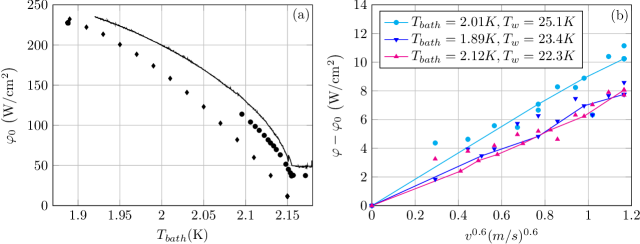
Figure 1: (a): Average heat flux at the surface of a hot wire of size $D_{w}=1.3\,\mathrm{\mu m}$ operated at $T_{w}\simeq 21K$ at null velocity. Continuous line: time series during cooling of the bath, obtained using a constant-resistance CTA electronics. Circles ($\bullet$): open loop constant voltage measurements (see text). Diamonds ($\blacklozenge$): Numerical integration of the model based on conduction function. (b): additional heat flux due to He II forced convection, represented as a function the power 0.6 of the velocity. The points that are linked by a line are the result of a 30 times longer averaging and their temperature is controlled much more carefully than unlinked points.

The observed velocity dependence of the heat flux $\varphi$ (averaged over the whole wire surface) can be written in the same form as in classical fluids:

$$\varphi=\varphi_{0}+Bv^{\alpha},$$ (2)

with $\alpha\simeq 0.5$ in the general case due to the $v^{-0.5}$ scaling of the thermal boundary layer thickness. While in He I data (not shown here), $\alpha=0.5$ is well suited, in He II case, a value $\alpha=0.6$ gives a slightly better fit (see figure 1(b)).

The probe response in He-II and its similarity with the response of classical hot wires are first indications that hot wires can be operated as velocity probes in He-II. Still, heat transfer processes occurring near the wire surface are more complex -as discussed later- and no clear justification can be brought about the slight change in the scaling with the mean flow velocity. Consequently, we have decided to analyze time series data of the raw CTA output $e(t)$ rather than attempting to use Eq. 2 to convert it into velocity time series. Since $\varphi\sim e(t)^{2}$ and $\varphi-\varphi_{0}\ll\varphi_{0}$, the fluctuations of the raw signal $e(t)$ are nearly proportional to the heat flux $\varphi-\varphi_{0}$.

III.2 Power spectra from the hot-wire

Figure 2 presents the power spectral density (PSD) of the voltage $e$ delivered by the hot wire electronics, normalized by its variance $\sigma_{e}^{2}$:

$$E^{*}(f)=E(f)/\sigma_{e}^{2},$$ (3)

where $E$, the PSD of the voltage signal, is computed using Welch periodogram method over windows of $2^{16}$ points. The PSD at four different temperatures, ranging from $1.76\,\mathrm{K}$ up to $2.12\,\mathrm{K}$ ($T<T_{\lambda}$), are represented as a function of the frequency for a mean flow velocity $U_{60D}=1.3\,\mathrm{m.s^{-1}}$ on the wire. Null jet velocity PSD are represented (filled symbols) normalized by the variance of their corresponding non-null-velocity signal. For comparison, the normalized PSD at null jet velocity in He I is also represented (pointing down triangles).

The first observation is that the null velocity “noise” has a much higher level of fluctuations in He II than in He I.

At non-null jet velocities, a Gaussian white PSD is observed up to $f\approx 2\,\mathrm{Hz}$. This is consistent with the expected incoherent motion of the very large scales of the flow. For higher frequencies, the PSD exhibit a power law behavior consistent with Kolmogorov $f^{-5/3}$ scaling. A departure from this power law is observed at frequencies of order $f\approx 2\,\mathrm{kHz}$, except at temperatures close to $T_{\lambda}$: the PSD decreases much less rapidly (roughly as $f^{-0.5}$). As can be seen, at the highest resolved frequencies, the energy density of the signal is always higher than the one observed at null velocity.

The observation of a plateau followed by a Kolmogorov-like spectra in He-II is a second indication that the hot wire is sensitive to velocity fluctuations, at least up to 2 kHz. Indeed, such spectral behavior have already been reported in He-II flows (e.g. Maurer and Tabeling (1998); Salort et al. (2010, 2012)) and their observation is known to be robust to non-linearities in the calibration law.

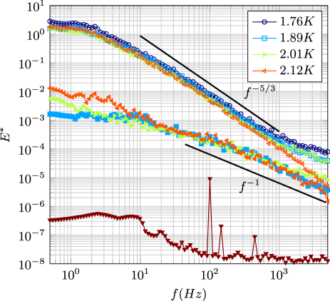
Figure 2: Power spectral density of the CTA electronics output voltage normalized by its variance, for a flow velocity $U_{60D}=1.3\,\mathrm{m.s^{-1}}$ (open symbols) at four temperatures. The corresponding colors with filled symbols correspond to the same temperature but at null velocity. In the latter case, the signal is normalized by the variance of the signal at non-null velocity. Pointing down triangles show the observed noise in He I (the corresponding non-null velocity spectrum is not shown here)

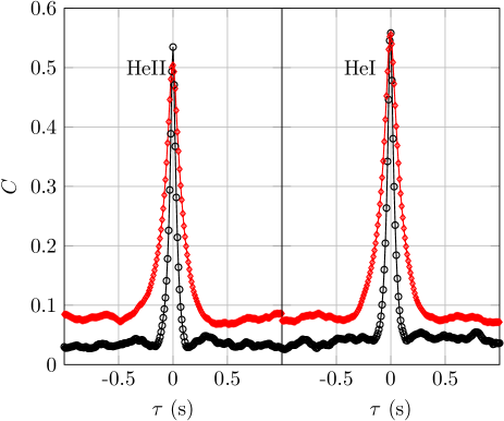
Figure 3: Cross-correlation coefficient of the hot wire signal and of a total head pressure tube situated 4 mm apart (black $\circ$ 1.72 m/s and red $\diamond$ 0.86 m/s, color online). Measurements are performed at 45 $D_{n}$ from the nozzle.

III.3 Correlation with a Pitot tube anemometer

A Pitot-tube anemometer working both in He-I and He-II was specially made to test the correlation between the raw hot-wire signal and velocity fluctuations. It is mounted close to the hot-wire, at a 4 mm transverse distance and 3 mm downstream of it. Its design is based on those found in Salort et al. (2010). Figures 3(a) and (b) present the cross-correlation $C(\tau)$ of the Pitot anemometer raw electrical signal $v(t)$ with the hot wire CTA raw output signal $e(t)$ both in He-I and He-II, where

$$C(\tau)=\frac{\langle(e(t)-\langle e\rangle)(v(t+\tau)-\langle v\rangle)\rangle}{\sigma_{e}\sigma_{v}},$$

$\sigma_{e}$ and $\sigma_{v}$ being the root-mean-squared values of the signals.

In He-I both probes are known to measure velocity. The maximum value of $C$ at small time lag, about 55% is not expected to be 100% because the hot-wire signal is not calibrated and its calibration curve is not expected to be linear. Furthermore, the noises of the sensors that have a non-hydrodynamic origin, are not expected to be correlated and will naturally decrease the correlation coefficient of the signals.

The most striking result is to obtain nearly the same level of correlation in He I and in He II. This gives a strong indication that the most energetic velocity fluctuations of the flow are producing similar response of the hot-wire in He-I -where it is a validated anemometer- and in He-II.

IV Discussion

IV.1 Response without external flow

Due to the 21 K operating temperature of the hot wire, the liquid helium in the vicinity of the wire surface is in the supercritical normal phase (noted He I hereafter for simplicity), while far from the wire, helium is in the He-II phase. These near-wire and far-wire regions are separated by an isotherm interface at $T_{\lambda}$. In the absence of external flow, we will first assume that the temperature distribution has a cylindrical symmetry, $r_{\lambda}$ being the radius of the $T_{\lambda}$ isotherm.

In the cylindrical shell of He-I surrounding the wire, molecular conduction is responsible for most of the heat transport . For a typical heat flux of $\varphi_{0}=100W.cm^{-2}$, numerical integration of Fourier law between $T_{w}\simeq 21K$ (at $r=D_{w}/2$) and $T_{\lambda}\simeq 2.15K$ (at $r=r_{\lambda}$) gives a He-I shell layer thickness of $r_{\lambda}-D_{w}/2\simeq 0.2\,\mathrm{\mu m}$. Although Fourier law may not be accurate over such a small distances and considering the very large temperature gradient, it still provides an estimate and shows that the He-I shell surrounding the wire is significantly thinner than the wire diameter.

In the far-wire region, molecular conduction is complemented by the counter-flow heat transport mechanism, specific to He-II Van Sciver (2012). At scales larger than the typical inter-vortex spacing, the overall mean heat flux in He-II is given by :

$$\tilde{\varphi}=\left(f(T,P)^{-1}\nabla T\right)^{1/m},$$ (4)

$m\simeq 3$ is the so-called Gorter-Mellink exponent (it was shown that $m$=3.4 generally leads to better fits of experimental dataSato et al. (2006); Bon Mardion, Claudet, and Seyfert (1979)) and $f(T,P)^{-1}$, called the conduction function, is a highly temperature and pressure dependent quantity which is null at $T_{\lambda}$ and maximum at $1.93\,\mathrm{K}$ in our experimental conditions.

The efficient heat transport brought by the counter-flow mechanism (Eq. 4) results in significantly smoother temperature gradients in He-II than in He-I (figure 4). The insert in figure 4 illustrates the dimensionless thermal boundary layer thickness $\delta_{T}/r_{\lambda}$ defined as $T(r_{\lambda}+\delta_{T})=(T_{bath}+T_{\lambda})/2$. As can be seen, the thermal boundary layer extends over a typical distance $\delta_{T}\simeq r_{\lambda}/5\simeq D_{w}/10$.

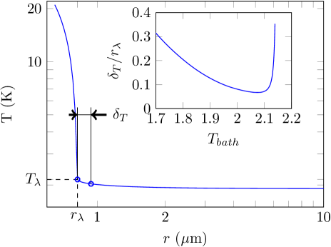
Figure 4: Typical radial temperature profile around the wire, computed for $T_{bath}=1.91$K. Insert: Thermal boundary layer in He II $\delta_{T}$ normalized by $r_{\lambda}$, the radius of He I region.

The conduction function is generally used for systems in which the heat flux is lower than in this experiment. In our case the very high heat flux leads to counter-flow velocities $v_{n}-v_{s}=\tilde{\varphi}/\rho_{s}ST$ that can be of order of the second sound velocity near the wire. For this reason, quantities extracted from the classical literature must be applied to our case with caution. However, it is interesting to use experimental (e.g. Tough (1982) and references there in) and numerical (e.g. Schwarz (1978)) fits to evaluate the superfluid vortex line density $\mathcal{L}_{0}(r)$ sustained by the counter-flow. Neglecting the mean velocity of the vortices in the tangle, the vortex line density can be estimated as:

$$\mathcal{L}_{0}=a\left(v_{n}-v_{s}\right)^{2}$$ (5)

where $a$ is a temperature dependent parameter. Using numerically computed values Schwarz (1978) of $a$, the maximum of $\mathcal{L}_{0}$ is found at $r=r_{\lambda}$, and represents an inter-vortex spacing of order $r_{\lambda}/50\simeq D_{w}/100$. This indicates that close to the wire, the inter-vortex spacing is much lower than the wire diameter. In first approximation, the time averaged vortex line density can be approximated as a continuous field at the wire diameter length scale, which thus justifies a posteriori the use of a continuous model to derive order of magnitude estimates.

Numerical integration of the model in He-I and He-II is done in cylindrical coordinates using Dirichlet boundary conditions:

$$\left\{\begin{array}[]{lcl}T=21\,\mathrm{K}&\mbox{for}&r=D_{w}/2=0.65\,\mathrm{\mu m}\\ T=T_{bath}&\mbox{for}&r=1000D_{w}\par\end{array}\right.$$

On figure 1(a) we have represented experimental (line and circles) and numerical (diamonds) heat flux $\varphi_{0}$ at the surface of the wire, as a function of the bath temperature $T_{bath}$. For temperatures well below $T_{\lambda}$, we find that our simple model accounts reasonably well both for the order of magnitude and temperature dependence of heat flux, showing that the underlying phenomena are mainly driven by the counter-flow mechanism. This is consistent with the previous studies with heated micro-wiresShiotsu, Hata, and Sakurai (1994); Ruzhu (1995), although they were done with wires with diameters 40 to 60 times larger. For bath temperatures $T_{bath}$ close to $T_{\lambda}$, our model predictions are underestimated by typically $50\,\mathrm{Wcm^{-2}}$. Since this offset is also present right above $T_{\lambda}$, it is not He-II related and its origin has not been examined in detail. Possible origins include thermal end-effect associated with the prongs or residual offset introduced by the circuitry. It should also be stressed out that the accuracy of our numerical simulation depends on the accuracy of the data we use for the conduction function: for a given temperature gradient, the computed flux using Hepak^® library (used for the numerical integration above) and correlations by Sato et al. (2006) differ by up to a factor of $\sim 2$ for large heat fluxes.

As a final remark, the observed heat flux without external flow in He II is a time dependent quantity, as illustrated by the PSD of figure 2 (filled symbols). Over 2 -3 decades, a $f^{-1}$ power law roughly fits the spectra. The fluctuating behavior of the heat flux in counter-flows was studied by various authors (for a review, see Nemirovskii and Fiszdon (1995)) and the cause of fluctuations is understood as turbulent nature of the counter-flow.

IV.2 Response to an external flow

In the previous section, we have presented three experimental results that can be interpreted stating that hot-wires can provide a direct measurement of velocity in He-II. Before discussing the velocity dependence, we first discuss (and finally discard) two alternative interpretations, namely the sensitivity to temperature fluctuations and to the vortex line density present in the external flow.

As stated above, the temperature sensitivity is of order $\tilde{\gamma}\approx-2\mathrm{K^{-1}}$. For the temperature driven fluctuations to contribute significantly to the measured signal, the temperature rms fluctuations $\delta T$ should be of order $\delta T=\left(\varphi(v)-\varphi_{0}\right)/(\varphi_{0}\tilde{\gamma})\approx 30\mathrm{mK}$ at the largest measured velocities. Such large temperature fluctuations are not likely to happen in our flow :

• At large time scales, i.e. for frequencies smaller than 10 Hz, the temperature controller maintains the temperature within $\pm 0.1\mathrm{mK}$. Furthermore, the correlation between the velocity and the temperature at large time scale is expected to be null because of the very efficient thermal transfer associated with He II.

• For smaller time scales, the local energy dissipation could produce temperature fluctuations but their order of magnitude would be much smaller. A higher bound for the dissipated energy by unit mass may be computed using the pressure loss through the nozzle which gives the maximum achievable temperature fluctuations in the flow : $\theta^{\prime}_{max}=V_{nozzle}^{2}/2Cp\approx 10\mathrm{mK}$, where $Cp$ is the constant pressure specific heat of helium. Once again the efficient thermalization of the flow due to the counter-flow prevents any such high temperature fluctuations at small time/length scales.

Thus, the temperature effect on the hot wire signal can reasonably be neglected, at least for the low frequency part of the signal.

Now the vortex line density $\mathcal{L}$ of the turbulent external flow could possibly contribute to the hot wire signal. Indeed, as mentioned earlier, the vortex lines are the basic ingredient limiting the heat flow in the counter-flow surrounding the wire and one could argue that the time-dependent vortex lines carried by the external flow will add up to the intrinsic vortex lines generated by the counter-flow. Here again two main arguments lead us to discard the relevance of this mechanism:

• The mean vortex spacing $\delta=\mathcal{L}^{-1/2}$ was found to behave similarly with the Kolmogorov dissipative scale in classical turbulence Salort, Roche, and Lévêque (2011); Babuin et al. (2014), i.e. $\mathcal{L}$ increases with the Reynolds number as $Re^{3/2}$ and thus with velocity. This leads to the conclusion that a higher mean velocity would lead to a degraded heat transfer, which is obviously opposite to the observation of Fig. 1-b.

• Both references cited above provide correlations between $\delta$ and the Reynolds number. In our conditions $\delta\approx 3\,\mathrm{\mu m}$ which is more than 100 times larger that the estimated value near the wire. The vortex line density of the external flow is much sparser than the one produced by the thermal counter-flow near the wire.

To discuss the velocity dependence, we first come back to the calibration law Eq. 2. Obviously the term $\varphi_{0}$ accounts for the heat flux at null velocity. In classical fluids this term is mainly due to natural convection whereas in He-II, it is due to the counter-flow mechanism, as seen previously. Contrary to the classical case, this null-velocity term in He-II is found to remain dominant over the advection term ($\varphi_{0}\gg Bv^{\alpha}$), even in the presence of a vigorous flow slightly exceeding $1\,\mathrm{ms^{-1}}$. Thus, it is reasonable to assume that the flow alters only slightly the underlying counterflow heat transport mechanism in most of the He-II fluid domain. A self consistency test of this assumption can be performed by estimating the local Péclet number defined as the ratio of the advection and counterflow terms

$$Pe(r)=\frac{\rho c_{p}v\left(T(r)-T_{bath}\right)}{\left(f(T,P)^{-1}\nabla T\right)^{1/m}},$$ (6)

where $\rho c_{p}$ is the volumetric heat capacity Van Sciver (2012). Numerical integration shows that $Pe$ remains smaller than one, in agreement with our assumption.

Solving the steady heat equation in He-II at null velocity gives $T(r)-T_{bath}\sim r^{1-m}$ for $r\gg r_{\lambda}+\delta_{T}$ (where $f(T,P)$ can be taken constant). Due to this pronounced power law decay ($1-m<-1$), the heat advected by the external flow in the far-wire region is small compared to the one advected in the wire vicinity, as can be seen by integration of the numerator of the $Pe(r)$. Thus, the velocity dependence of the heat transfer must originate from the near-wire region, say within few $r_{\lambda}+\delta_{T}\simeq 1\mu m$ from the wire axis. This analysis justifies the sensitivity to local fluctuations of the velocity, a key property of classical hot wires.

Modeling what happens in the micron-size region which surrounds the wire, and understanding the resulting velocity dependence is delicate and is beyond the scope of this experimental work. Difficulties arises because this near-wire region embraces a He-I classical fluid domain surrounded by the He-II superfluid and, on top of both the velocity boundary layer produced by the incoming flow impinging the wire. Additional technical difficulties arise from the strong fluid property variations in space, a possible breakdown of the validity of the continuous model, as well as a spatial cross-over from a radial counter-flow around the wire to a translational motion of He-II away from it.

As a final comment, we want to stress the small -if any- temperature dependence of the advection term $Bv^{\alpha}$ in the hot-wire calibration (see Fig. 1.b). This experimental result is very constraining for model development. For example, it undermines a straightforward modeling approach consisting in considering advection as an independent heat transport mechanism which adds up to an underlying counter-flow transport. Indeed, simple models elaborated along this line by integrating the advection term $\rho c_{p}v\left(T(r)-T_{bath}\right)$ using a classical velocity boundary layer successfully predict a $\sim v^{0.5}$ velocity-dependent heat transfer around the hot-wire but over-estimate significantly the temperature dependence of the advection term.

V Conclusion

We have brought three experimental observations, and presented quantitative arguments, that show that a hot-wire can be used as a local velocity sensor in He II turbulent flows.

We showed that the calibration law (against the mean velocity) shares some common scalings with the one observed in classical fluids. The good correlation of the hot-wire signal with a validated local velocity sensor together with the $f^{-5/3}$ scaling of the power spectra are further indications that the response of the hot-wire in He II is mainly related to the local velocity of the fluid.

The microscopic mechanisms near the surface of the wire when submitted to an external flow are delicate to analyze for a number of reasons listed above. Still, we could justify that the observed velocity dependence originates in the near vicinity of the wire, within typically one micron. Thus, the very high effective conductivity of He-II does not spoil the spatial resolution of the sensor.

Although further studies are needed to understand the microscopic physics at play within the micron-thick shell surrounding the hot-wire, such probe can already be counted as local velocity sensor in superfluid helium.

V.1 Acknowledgment

We would like to thank J. Salort for the design and implementation of the Pitot tubes used in preliminary studies. We also acknowledge J. Duplat and B. Rousset for fruitful discussions and P. Charvin for technical support. This work was supported by the French National Research Agency grant ANR-09-BLAN-0094-01 and by the European Community Framework Programme 7, EuHIT - European High-performance Infrastructures in Turbulence, grant agreement no. 312778.

References

- Van Sciver (2012) S. Van Sciver, Helium Cryogenics, International Cryogenics Monograph Series (Springer, 2012).
- Vinen and Niemela (2002) W. F. Vinen and J. J. Niemela, “Quantum turbulence,” Journal of Low Temperature Physics 128, 167–231 (2002).
- Barenghi, Skrbek, and Sreenivasan (2014) C. F. Barenghi, L. Skrbek, and K. R. Sreenivasan, “Introduction to quantum turbulence,” PNAS 111, 4647–4652 (2014).
- Barenghi, L’vov, and Roche (2014) C. F. Barenghi, V. S. L’vov, and P.-E. Roche, “Experimental, numerical, and analytical velocity spectra in turbulent quantum fluid,” PNAS 111, 4683–4690 (2014).
- Maurer and Tabeling (1998) J. Maurer and P. Tabeling, “Local investigation of superfluid turbulence,” Europhys. Lett. 43 (1), 29 (1998).
- Salort et al. (2010) J. Salort, C. Baudet, B. Castaing, B. Chabaud, F. Daviaud, T. Didelot, P. Diribarne, B. Dubrulle, Y. Gagne, F. Gauthier, et al., “Turbulent velocity spectra in superfluid flows,” Physics of Fluids 22, 5102 (2010).
- Salort et al. (2012) J. Salort, B. Chabaud, E. Lévêque, P.-E. Roche, et al., “Energy cascade and the four-fifths law in superfluid turbulence,” Europhysics Letters 97 (2012).
- Salort, Monfardini, and Roche (2012) J. Salort, A. Monfardini, and P.-E. Roche, “Cantilever anemometer based on a superconducting micro-resonator: Application to superfluid turbulence,” Review of Scientific Instruments 83, 125002 (2012).
- Murakami, Yamazaki, and Nakai (1989) M. Murakami, T. Yamazaki, and H. Nakai, “Laser doppler velocimeter measurements of thermal counterflow jet in he {II},” Cryogenics 29, 1143 – 1147 (1989).
- Zhang and Van Sciver (2004) T. Zhang and S. Van Sciver, “Use of the particle image velocimetry technique to study the propagation of second sound shock in superfluid helium,” Physics of Fluids 16, L99–L102 (2004).
- Bewley, Lathrop, and Sreenivasan (2006) G. P. Bewley, D. P. Lathrop, and K. R. Sreenivasan, “Superfluid helium: Visualization of quantized vortices,” Nature 441, 588–588 (2006).
- La Mantia et al. (2013) M. La Mantia, D. Duda, M. Rotter, and L. Skrbek, “Lagrangian accelerations of particles in superfluid turbulence,” Journal of Fluid Mechanics 717, R9 (2013).
- Chanal et al. (2000) O. Chanal, B. Chabaud, B. Castaing, and B. Hébral, “Intermittency in a turbulent low temperature gaseous helium jet,” The European Physical Journal B-Condensed Matter and Complex Systems 17, 309–317 (2000).
- Bailey et al. (2010) S. C. Bailey, G. J. Kunkel, M. Hultmark, M. Vallikivi, J. P. Hill, K. A. Meyer, C. Tsay, C. B. Arnold, and A. J. Smits, “Turbulence measurements using a nanoscale thermal anemometry probe,” Journal of Fluid Mechanics 663, 160–179 (2010).
- Moisy, Tabeling, and Willaime (1999) F. Moisy, P. Tabeling, and H. Willaime, “Kolmogorov equation in a fully developed turbulence experiment,” Physical Review Letters 82, 3994–3997 (1999).
- Pietropinto et al. (2003) S. Pietropinto, C. Poulain, C. Baudet, B. Castaing, B. Chabaud, Y. Gagne, B. Hébral, Y. Ladam, P. Lebrun, O. Pirotte, and P.-E. Roche, “Superconducting instrumentation for high reynolds turbulence experiments with low temperature gaseous helium,” Physica C 386, 512 (2003).
- Quix and Quest (2012) H. Quix and J. Quest, “Hotwires in pressurized, cryogenic environment - it works!” in 50th AIAA Aerospace Sciences Meeting including the New Horizons Forum and Aerospace Exposition (American Institute of Aeronautics and Astronautics, 2012).
- Vinen (2010) W. F. Vinen, “Quantum turbulence: Achievements and challenges,” Journal of Low Temperature Physics 161, 419–444 (2010).
- Johnson and Jones (1978) W. Johnson and M. Jones, “Measurements of axial heat transport in helium ii with forced convection,” in Advances in Cryogenic Engineering, Advances in Cryogenic Engineering, Vol. 23 (Springer US, 1978) pp. 363–370.
- Barenghi, Donnelly, and Vinen (2001) C. F. Barenghi, R. J. Donnelly, and W. Vinen, Quantized vortex dynamics and superfluid turbulence, Vol. 571 (Springer, 2001).
- Duri et al. (2011) D. Duri, C. Baudet, P. Charvin, J. Virone, B. Rousset, J. Poncet, and P. Diribarne, “Liquid helium inertial jet for comparative study of classical and quantum turbulence,” Review of Scientific Instruments 82 (2011).
- Wygnanski and Fiedler (1969) I. J. Wygnanski and H. E. Fiedler, “Some measurements in the self-preserving jet,” Journal of Fluid Mechanics 38, 577–612 (1969).
- Note (1) Comparatively, radiative heat transfer is inefficient due to its scaling, as well as natural convection due to the thinness of the He-I shell . Indeed, all Grashof numbers assessed are found significantly lower than unity, regardless of the chosen fluid properties over the interval .
- Sato et al. (2006) A. Sato, M. Maeda, T. Dantsuka, M. Yuyama, and Y. Kamioka, “Temperature Dependence of the Gorter-Mellink Exponent m Measured in a Channel Containing He II,” in Advances in Cryogenic Engineering: Transactions of the Cryogenic Engineering Conference, Vol. 823 (2006) pp. 387–392.
- Bon Mardion, Claudet, and Seyfert (1979) G. Bon Mardion, G. Claudet, and P. Seyfert, “Practical data on steady state heat transport in superfluid helium at atmospheric pressure,” Cryogenics 19, 45 – 47 (1979).
- Tough (1982) J. Tough, “Superfluid turbulence,” Progress in low temperature physics 8, 133 (1982).
- Schwarz (1978) K. Schwarz, “Turbulence in superfluid helium: Steady homogeneous counterflow,” Physical Review B 18, 245 (1978).
- Shiotsu, Hata, and Sakurai (1994) M. Shiotsu, K. Hata, and A. Sakurai, “Effect of test heater diameter on critical heat flux in he ii,” in Advances in Cryogenic Engineering, Vol. 39, edited by P. Kittel (Plenum Press, New York, 1994) pp. 1797–1804.
- Ruzhu (1995) W. Ruzhu, “Measurement of steady state heat transfer in a bath of sub-cooled superfluid helium,” Journal of Physics D: Applied Physics 28, 25 (1995).
- Nemirovskii and Fiszdon (1995) S. K. Nemirovskii and W. Fiszdon, “Chaotic quantized vortices and hydrodynamic processes in superfluid helium,” Rev. Modern Phys. 67, 37–84 (1995).
- Note (2) To the best of our knowledge, only spectral measurements of the vortex line density have been reported previously. In particular, Ref. Tough (1982) reports vortex line density fluctuations spectra with a power law followed, after a cut-off frequency, by a power law. In this previous experiment, the cut off frequency increases with the heat flux and is thus expected to be very high in our experiment where the heat flux is times higher. The spectra that we measured is therefore expected to correspond to the vortex line density spectra.
- Salort, Roche, and Lévêque (2011) J. Salort, P.-E. Roche, and E. Lévêque, “Mesoscale equipartition of kinetic energy in quantum turbulence,” EPL 94, 24001 (2011).
- Babuin et al. (2014) S. Babuin, E. Varga, L. Skrbek, E. Lévêque, and P.-E. Roche, “Effective viscosity in quantum turbulence: A steady-state approach,” EPL (Europhysics Letters) 106, 24006 (2014).