Instrumental Variables: An Econometrician’s Perspective

Abstract

I review recent work in the statistics literature on instrumental variables methods from an econometrics perspective. I discuss some of the older, economic, applications including supply and demand models and relate them to the recent applications in settings of randomized experiments with noncompliance. I discuss the assumptions underlying instrumental variables methods and in what settings these may be plausible. By providing context to the current applications, a better understanding of the applicability of these methods may arise.

FLA

T1Discussed in d10.1214/14-STS494, d10.1214/14-STS485, d10.1214/14-STS488, d10.1214/14-STS491; rejoinder at r10.1214/14-STS496.

1 Introduction

Instrumental Variables (IV) refers to a set of methods developed in econometrics starting in the 1920s to draw causal inferences in settings where the treatment of interest cannot be credibly viewed as randomly assigned, even after conditioning on additional covariates, that is, settings where the assumption of no unmeasured confounders does not hold. In the last two decades, these methods have attracted considerable attention in the statistics literature. Although this recent statistics literature builds on the earlier econometric literature, there are nevertheless important differences. First, the recent statistics literature primarily focuses on the binary treatment case. Second, the recent literature explicitly allows for treatment effect heterogeneity. Third, the recent instrumental variables literature (starting with Imbens and Angrist (1994); Angrist, Imbens and Rubin (1996); Heckman (1990); Manski (1990); and Robins (1986)) explicitly uses the potential outcome framework used by Neyman for randomized experiments and generalized to observational studies by Rubin (1974, 1978, 1990). Fourth, in the applications this literature has concentrated on, including randomized experiments with noncompliance, the intention-to-treat or reduced-form estimates are often of greater interest than they are in the traditional econometric simultaneous equations applications.

Partly the recent statistics literature has been motivated by the earlier econometric literature on instrumental variables, starting with Wright (1928) (see the discussion on the origins of instrumental variables in Stock and Trebbi (2003)). However, there are also other antecedents, outside of the traditional econometric instrumental variables literature, notably the work by Zelen on encouragement designs (Zelen, 1979, 1990). Early papers in the recent statistics literature include Angrist, Imbens and Rubin (1996), Robins (1989) and McClellan and Newhouse (1994). Recent reviews include Rosenbaum (2010), Vansteelandt et al. (2011) and Hernán and Robins (2006). Although these reviews include many references to the earlier economics literature, it might still be useful to discuss the econometric literature in more detail to provide some background and perspective on the applicability of instrumental variables methods in other fields. In this discussion, I will do so.

Instrumental variables methods have been a central part of the econometrics canon since the first half of the twentieth century, and continue to be an integral part of most graduate and undergraduate textbooks (e.g., Angrist and Pischke, 2009; Bowden and Turkington (1984); Greene (2011); Hayashi (2000); Manski (1995); Stock and Watson (2010); Wooldridge, 2010, 2008). Like the statisticians Fisher and Neyman (Fisher (1925); Splawa-Neyman, 1990), early econometricians such as Wright (1928), Working (1927), Tinbergen (1930) andHaavelmo (1943) were interested in drawing causal inferences, in their case about the effect of economic policies on economic behavior. However, in sharp contrast to the statistical literature on causal inference, the starting point for these econometricians was not the randomized experiment. From the outset, there was a recognition that in the settings they studied, the causes, or treatments, were not assigned to passive units (economic agents in their setting, such as individuals, households, firms or countries). Instead the economic agents actively influence, or even explicitly choose, the level of the treatment they receive. Choice, rather than chance, was the starting point for thinking about the assignment mechanism in the econometrics literature. In this perspective, units receiving the active treatment are different from those receiving the control treatment not just because of the receipt of the treatment: they (choose to) receive the active treatment because they are different to begin with. This makes the treatment potentially endogenous, and creates what is sometimes in the econometrics literature referred to as the selection problem (Heckman (1979)).

The early econometrics literature on instrumental variables did not have much impact on thinking in the statistics community. Although some of the technical work on large sample properties of various estimators did get published in statistics journals (e.g., the still influential Anderson and Rubin, 1949 paper), applications by noneconomists were rare. It is not clear exactly what the reasons for this are. One possibility is the fact that the early literature on instrumental variables was closely tied to substantive economic questions (e.g., interventions in markets), using theoretical economic concepts that may have appeared irrelevant or difficult to translate to other fields (e.g., supply and demand). This may have suggested to noneconomists that the instrumental variables methods in general had limited applicability outside of economics. The use of economic concepts was not entirely unavoidable, as the critical assumptions underlying instrumental variables methods are substantive and require subtle subject matter knowledge. A second reason may be that although the early work by Tinbergen and Haavelmo used a notation that is very similar to what Rubin (1974) later called the potential outcome notation, quickly the literature settled on a notation only involving realized or observed outcomes; see for a historial perspective Hendry and Morgan (1992) and Imbens (1997). This realized-outcome notation that remains common in the econometric textbooks obscures the connections between the Fisher and Neyman work on randomized experiments and the instrumental variables literature. It is only in the 1990s that econometricians returned to the potential outcome notation for causal questions (e.g., Heckman (1990); Manski (1990); Imbens and Angrist (1994)), facilitating and initiating a dialogue with statisticians on instrumental variable methods.

The main theme of the current paper is that the early work in econometrics is helpful in understanding the modern instrumental variables literature, and furthermore, is potentially useful in improving applications of these methods and identifying potential instruments. These methods may in fact be useful in many settings statisticians study. Exposure to treatment is rarely solely a matter of chance or solely a matter of choice. Both aspects are important and help to understand when causal inferences are credible and when they are not. In order to make these points, I will discuss some of the early work and put it in a modern framework and notation. In doing so, I will address some of the concerns that have been raised about the applicability of instrumental variables methods in statistics. I will also discuss some areas where the recent statistics literature has extended and improved our understanding of instrumental variables methods. Finally, I will review some of the econometric terminology and relate it to the statistical literature to remove some of the semantic barriers that continue to separate the literatures. I should emphasize that many of the topics discussed in this review continue to be active research areas, about which there is considerable controversy both inside and outside of econometrics.

The remainder of the paper is organized as follows. In Section 2, I will discuss the distinction between the statistics literature on causality with its primary focus on chance, arising from its origins in the experimental literature, and the econometrics or economics literature with its emphasis on choice. The next two sections discuss in detail two classes of examples. In Section 3, I discuss the canonical example of instrumental variables in economics, the estimation of supply and demand functions. In Section 4, I discuss a modern class of examples, randomized experiments with noncompliance. In Section 5, I discuss the substantive content of the critical assumptions, and in Section 6, I link the current literature to the older textbook discussions. In Section 7, I discuss some of the recent extensions of traditional instrumental variables methods. Section 8 concludes.

2 Choice versus Chance in Treatment Assignment

Although the objectives of causal analyses in statistics and econometrics are very similar, traditionally statisticians and economists have approached these questions very differently. A key difference in the approaches taken in the statistical and econometric literatures is the focus on different assignment mechanisms, those with an emphasis on chance versus those with an emphasis on choice. Although in practice in many observational studies assignment mechanisms have elements of both chance and choice, the traditional starting points in the two literatures are very different, and it is only recently that these literatures have discovered how much they have in common.

2.1 The Statistics Literature: The Focus on Chance

The starting point in the statistics literature, going back to Fisher (1925) and Splawa-Neyman (1990), is the randomized experiment, with both Fisher and Neyman motivated by agricultural applications where the units of analysis are plots of land. To be specific, suppose we are interested in the average causal effect of a binary treatment or intervention, say fertilizer $A$ or fertilizer $B$, on plot yields. In the modern notation and language originating with Rubin (1974), the unit (plot) level causal effect is a comparison between the two potential outcomes, $Y_{i}(A)$ and $Y_{i}(B)$ [e.g., the difference $\tau_{i}=Y_{i}(B)-Y_{i}(A)$], where $Y_{i}(A)$ is the potential outcome given fertilizer $A$ and $Y_{i}(B)$ is the potential outcome given fertilizer $B$, both for plot $i$. In a completely randomized experiment with $N$ plots, we select $M$ (with $M\in\{1,\ldots,N-1\}$) plots at random to receive fertilizer $B$, with the remaining $N-M$ plots assigned to fertilizer $A$. Thus, the treatment assignment, denoted by $X_{i}\in\{A,B\}$ for plot $i$, is by design independent of the potential outcomes. In this specific setting, the work by Fisher and Neyman shows how one can draw exact causal inferences. Fisher focused on calculating exact $p$-values for sharp null hypotheses, typically the null hypothesis of no effect whatsoever, $Y_{i}(A)=Y_{i}(B)$ for all plots. Neyman focused on developing unbiased estimators for the average treatment effect $\sum_{i}(Y_{i}(A)-Y_{i}(B))/N$ and the variance of those estimators.

The subsequent literature in statistics, much of it associated with the work by Rubin and coauthors (Cochran (1968); Cochran and Rubin (1973); Rubin, 1974, 1990, 2006; Rosenbaum and Rubin, 1983; Rubin and Thomas (1992); Rosenbaum, 2002, 2010; Holland (1986)) has focused on extending and generalizing the Fisher and Neyman results that were derived explicitly for randomized experiments to the more general setting of observational studies. A large part of this literature focuses on the case where the researcher has additional background information available about the units in the study. The additional information is in the form of pretreatment variables or covariates not affected by the treatment. Let $V_{i}$ denote these covariates. A key assumption in this literature is that conditional on these pretreatment variables the assignment to treatment is independent of the treatment assignment. Formally,

$$X_{i}\perp\bigl{(}Y_{i}(A),Y_{i}(B)\bigr{)}|V_{i}\quad\mbox{(unconfoundedness)}.$$

Following Rubin (1990), I refer to this assumption as unconfoundedness given $V_{i}$, also known as no unmeasured confounders. This assumption, in combination with the auxiliary assumption that for all values of the covariates the probability of being assigned to each level of the treatment is strictly positive is referred to as strong ignorability (Rosenbaum and Rubin, 1983). If we assume only that $X_{i}\perp Y_{i}(A)|V_{i}$ and $X_{i}\perp Y_{i}(B)|V_{i}$ rather than jointly, the assumption is referred to as weak unconfoundedness (Imbens (2000)), and the combination as weak ignorability. Substantively, it is not clear that there are cases in the setting with binary treatments where the weak version is plausible but not the strong version, although the difference between the two assumptions has some content in the multivalued treatment case (Imbens (2000)). In the econometric literature, closely related assumptions are referred to as selection-on-observables (Barnow, Cain and Goldberger (1980)) or exogeneity.

Under weak ignorability (and thus also under strong ignorability), it is possible to estimate precisely the average effect of the treatment in large samples. In other words, the average effect of the treatment is identified. Various specific methods have been proposed, including matching, subclassification and regression. See Rosenbaum (2010), Rubin (2006), Imbens (2004, 2014), Gelman and Hill (2006), Imbens and Rubin (2014) and Angrist and Pischke (2009) for general discussions and surveys. Robins and coauthors (Robins (1986); Gill and Robins (2001); Richardson and Robins (2013); Van der Laan and Robins, 2003) have extended this approach to settings with sequential treatments.

2.2 The Econometrics Literature: The Focus on Choice

In contrast to the statistics literature whose point of departure was the randomized experiment, the starting point in the economics and econometrics literatures for studying causal effects emphasizes the choices that led to the treatment received. Unlike the original applications in statistics where the units are passive, for example, plots of land, with no influence over their treatment exposure, units in economic analyses are typically economic agents, for example, individuals, families, firms or administrations. These are agents with objectives and the ability to pursue these objectives within constraints. The objectives are typically closely related to the outcomes under the various treatments. The constraints may be legal, financial or information-based.

The starting point of economic science is to model these agents as behaving optimally. More specifically, this implies that economists think of everyone of these agents as choosing the level of the treatment to most efficiently pursue their objectives given the constraints they face. In practice, of course, there is often evidence that not all agents behave optimally. Nevertheless, the starting point is the presumption that optimal behavior is a reasonable approximation to actual behavior, and the models economists take to the data often reflect this.

2.3 Some Examples

Let us contrast the statistical and econometric approaches in a highly stylized example. Roy (1951) studies the problem of occupational choice and the implications for the observed distribution of earnings. He focuses on an example where individuals can choose between two occupations, hunting and fishing. Each individual has a level of productivity associated with each occupation, say, the total value of the catch per day. For individual $i$, the two productivity levels are $Y_{i}(h)$ and $Y_{i}(f)$, for the productivity level if hunting and fishing, respectively. Suppose the researcher is interested in the average difference in productivity in these two occupations, $\tau=\mathbb{E}[Y_{i}(f)-Y_{i}(h)]$, where the averaging is over the population of individuals. The researcher observes for all units in the sample the occupation they chose ($X_{i}$, equal to $h$ for hunters and $f$ for fishermen) and the productivity in their chosen occupation,

$$Y_{i}^{\mathrm{obs}}=Y_{i}(X_{i})=\cases{Y_{i}(h)&$\mbox{if }X_{i}=h$,\vspace*{2pt}\cr Y_{i}(f)&$\mbox{if }X_{i}=f$.}$$

In the Fisher–Neyman–Rubin statistics tradition, one might start by estimating $\tau$ by comparing productivity levels by occupation:

$$\hat{\tau}=\overline{Y}^{\mathrm{obs}}_{f}-\overline{Y}^{\mathrm{obs}}_{h},$$

where

$$\overline{Y}^{\mathrm{obs}}_{f} = \frac{1}{N_{f}}\sum_{i:X_{i}=f}Y^{\mathrm{obs}}_{i},\quad\overline{Y}^{\mathrm{obs}}_{h}=\frac{1}{N_{h}}\sum_{i:X_{i}=h}Y^{\mathrm{obs}}_{i},$$

$$N_{f} = \sum_{i=1}^{N}\mathbf{1}_{X_{i}=f}\quad\mbox{and}\quad N_{h}=N-N_{f}.$$

If there is concern that these unadjusted differences are not credible as estimates of the average causal effect, the next step in this approach would be to adjust for observed individual characteristics such as education levels or family background. This would be justified if individuals can be thought of as choosing, at least within homogenous groups defined by covariates, randomly which occupation to engage in.

Roy, in the economics tradition, starts from a very different place. Instead of assuming that individuals choose their occupation (possibly after conditioning on covariates) randomly, he assumes that each individual chooses her occupation optimally, that is, the occupation that maximizes her productivity:

$$X_{i}=\cases{f&$\mbox{if }Y_{i}(f)\geq Y_{i}(h)$,\cr h&$\mbox{otherwise}$.}$$

There need not be a solution in all cases, especially if there is interference, and thus there are general equilibrium effects, but I will assume here that such a solution exists. If this assumption about the occupation choice were strictly true, it would be difficult to learn much about $\tau$ from data on occupations and earnings. In the spirit of research by Manski (1990, 2000b, 2001), Manski and Pepper (2000), and Manski et al. (1992), one can derive bounds on $\tau$, exploiting the fact that if $X_{i}=f$, then the unobserved $Y_{i}(h)$ must satisfy $Y_{i}(h)\leq Y_{i}(f)$, with $Y_{i}(f)$ observed. For the Roy model, the specific calculations have been reported in Manski (1995), Section 2.6. Without additional information or restrictions, these bounds might be fairly wide, and often one would not learn much about $\tau$. However, the original version of the Roy model, where individuals know ex ante the exact value of the potential outcomes and choose the level of the treatment corresponding to the maximum of those, is ultimately not plausible in practice. It is likely that individuals face uncertainty regarding their future productivity, and thus may not be able to choose the ex post optimal occupation; see for bounds under that scenario Manski and Nagin (1998). Alternatively, and this is emphasized in Athey and Stern (1998), individuals may have more complex objective functions taking into account heterogenous costs or nonmonetary benefits associated with each occupation. This creates a wedge between the outcomes that the researcher focuses on and the outcomes that the agent optimizes over. What is key here in relation to the statistics literature is that under the Roy model and its generalizations the very fact that two individuals have different occupations is seen as indicative that they have different potential outcomes, thus fundamentally calling into question the unconfoundedness assumption that individuals with similar pretreatment variables but different treatment levels are comparable. This concern about differences between individuals with the same values for pretreatment variables but different treatment levels underlies many econometric analyses of causal effects, specifically in the literature on selection models. See Heckman and Robb (1985) for a general discussion.

Let me discuss two additional examples. There is a large literature in economics concerned with estimating the causal effect of educational achievement (measured as years of education) on earnings; see for general discussions Griliches (1977) and Card (2001). One starting point, and in fact the basis of a large empirical literature, is to compare earnings for individuals who look similar in terms of background characteristics, but who differ in terms of educational achievement. The concern in an equally large literature is that those individuals who choose to acquire higher levels of education did so precisely because they expected their returns to additional years of education to be higher than individuals who choose not to acquire higher levels of education expected their returns to be. In the terminology of the returns-to-education literature, the individuals choosing higher levels of education may have higher levels of ability, which lead to higher earnings for given levels of education.

Another canonical example is that of voluntary job training programs. One approach to estimate the causal effect of training programs on subsequent earnings would be to compare earnings for those participating in the program with earnings for those who did not. Again the concern would be that those who choose to participate did so because they expected bigger benefits (financial or otherwise) from doing so than individuals who chose not to participate.

These issues also arise in the missing data literature. The statistics literature (Rubin, 1976, 1987, 1996; Little and Rubin, 1987) has primarily focused on models that assume that units with item nonresponse are comparable to units with complete response, conditional on covariates that are always observed. The econometrics literature (Heckman, 1976, 1979) has focused more heavily on models that interpret the nonresponse as the result of systematic differences between units. Philipson (1997a, 1997b), Philipson and DeSimone (1997), and Philipson and Hedges (1998) take this even further, viewing survey response as a market transaction, where individuals not responding the survey do so deliberately because the costs of responding outweighs the benefits to these nonrespondents. The Heckman-style selection models often assume strong parametric alternatives to the Little and Rubin missing-at-random or ignorability condition. This has often in turn led to estimators that are sensitive to small changes in the data generating process. See Little (1985).

These issues of nonrandom selection are of course not special to economics. Outside of randomized experiments, the exposure to treatment is typically also chosen to achieve some objectives, rather than randomly within homogenous populations. For example, physicians presumably choose treatments for their patients optimally, given their knowledge and given other constraints (e.g., financial). Similarly, in economics and other social sciences one may view individuals as making optimal decisions, but these are typically made given incomplete information, leading to errors that may make the ultimate decisions appear as good as random within homogenous subpopulations. What is important is that the starting point is different in the two disciplines, and this has led to the development of substantially different methods for causal inference.

2.4 Instrumental Variables

How do instrumental variables methods address the type of selection issues the Roy model raises? At the core, instrumental variables change the incentives for agents to choose a particular level of the treatment, without affecting the potential outcomes associated with these treatment levels. Consider a job training program example where the researcher is interested in the average effect of the training program on earnings. Each individual is characterized by two potential earnings outcomes, earnings given the training and earnings in the absence of the training. Each individual chooses to participate or not based on their perceived net benefits from doing so. As pointed out in Athey and Stern (1998), it is important that these net benefits that enter into the individual’s decision differ from the earnings that are the primary outcome of interest to the researcher. They do so by the costs associated with participating in that regime. Suppose that there is variation in the costs individuals incur with participation in the training program. The costs are broadly defined, and may include travel time to the program facilities, or the effort required to become informed about the program. Furthermore, suppose that these costs are independent of the potential outcomes. This is a strong assumption, often made more plausible by conditioning on covariates. Measures of the participation cost may then serve as instrument variables and aid in the identification of the causal effects of the program. Ultimately, we compare earnings for individuals with low costs of participation in the program with those for individuals with high costs of participation and attribute the difference in average earnings to the increased rate of participation in the program among the two groups.

In almost all cases, the assumption that there is no direct effect of the change in incentives on the potential outcomes is controversial, and it needs to be assessed at a case-by-case level. The second part of the assumption, that the costs are independent of the potential outcomes, possibly after conditioning on covariates, is qualitatively very different. In some cases, it is satisfied by design, for example, if the incentives are randomized. In observational studies, it is a substantive, unconfoundedness-type, assumption, that may be more plausible or at least approximately hold after conditioning on covariates. For example, in a number of studies researchers have used physical distance to facilities as instruments for exposure to treatments available at such facilities. Such studies include McClellan and Newhouse (1994) and Baiocchi et al. (2010) who use distance to hospitals with particular capabilities as an instrument for treatments associated with those capabilities, after conditioning on distance to the nearest medical facility, and Card (1995), who uses distance to colleges as an instrument for attending college.

3 The Classic Example: Supply and Demand

In this section, I will discuss the classic example of instrumental variables methods in econometrics, that is, simultaneous equations. Simultaneous equations models are both at the core of the econometrics canon and at the core of the confusion concerning instrumental variables methods in the statistics literature. More precisely, in this section I will look at supply and demand models that motivated the original research into instrumental variables. Here, the endogeneity, that is, the violation of unconfoundedness, arises from an equilibrium condition. I will discuss the model in a very specific example to make the issues clear, as I think that perhaps the level of abstraction used in the older econometric text books has hampered communication with researchers in other fields.

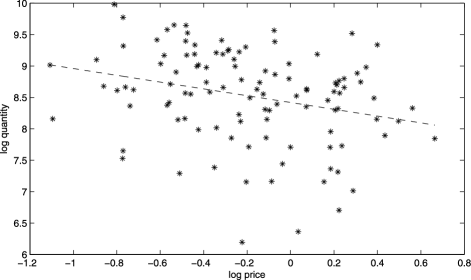
Figure 1: Scatterplot of log prices and log quantities.

3.1 Discussions in the Statistics Literature

To show the level of frustration and confusion in the statistics literature with these models, let me present some quotes. In a comment on Pratt and Schlaifer (1984), Dawid (1984) writes “I despair of ever understanding the logic of simultaneous equations well enough to tackle them,” (page 24). Cox (1992) writes in a discussion on causality “it seems reasonable that models should be specified in a way that would allow direct computer simulation of the data$\ldots$ . This, for example, precludes the use of $y_{2}$ as an explanatory variable for $y_{1}$ if at the same time $y_{1}$ is an explanatory variable for $y_{2}$” (page 294). This restriction appears to rule out the first model Haavelmo considers, that is, equations (1.1) and (1.2) (Haavelmo (1943), page 2):

$$Y=aX+\epsilon_{1},\quad X=bY+\epsilon_{2}$$

(see also Haavelmo, 1944). In fact, the comment by Cox appears to rule out all simultaneous equations models of the type studied by economists. Holland (1988), in comment on structural equation methods in econometrics, writes “why should [this disturbance] be independent of [the instrument]$\ldots$ when the very definition of [this disturbance] involves [the instrument],” (page 460). Freedman writes “Additionally, some variables are taken to be exogenous (independent of the disturbance terms) and some endogenous (dependent on the disturbance terms). The rationale is seldom clear, because—among other things—there is seldom any very clear description of what the disturbance terms mean, or where they come from” (Freedman (2006), page 699).

3.2 The Market for Fish

The specific example I will use in this section is the market for whiting (a particular white fish, often used in fish sticks) traded at the Fulton fish market in New York City. Whiting was sold at the Fulton fish market at the time by a small number of dealers to a large number of buyers. Kathryn Graddy collected data on quantities and prices of whiting sold by a particular trader at the Fulton fish market on 111 days between December 2, 1991, and May 8, 1992 (Graddy, 1995, 1996; Angrist, Graddy and Imbens (2000)). I will take as the unit of analysis a day, and interchangeably refer to this as a market. Each day, or market, during the period covered in this data set, indexed by $t=1,\ldots,111$, a number of pounds of whiting are sold by this particular trader, denoted by $Q_{t}^{\mathrm{obs}}$. Not every transaction on the same day involves the same price, but to focus on the essentials I will aggregate the total amount of whiting sold and the total amount of money it was sold for, and calculate a price per pound (in cents) for each of the 111 days, denoted by $P_{t}^{\mathrm{obs}}$. Figure 1 presents a scatterplot of the observed log price and log quantity data. The average quantity sold over the 111 days was 6335 pounds, with a standard deviation of 4040 pounds, for an average of the average within-day prices of 88 cts per pound and a standard deviation of 34 cts. For example, on the first day of this period 8058 pounds were sold for an average of 65 cents, and the next day 2224 pounds were sold for an average of 100 cents. Table 1 presents averages of log prices and log quantities for the fish data.

=13.5cm Logarithm of price Logarithm of quantity     Number of observations Average Standard deviation Average Standard deviation All $111$ $-0.19$ (0.38) 8.52 (0.74) Stormy $32$ $0.04$ (0.35) 8.27 (0.71) Not-stormy $79$ $-0.29$ (0.35) 8.63 (0.73) Stormy $32$ $0.04$ (0.35) 8.27 (0.71) Mixed $34$ $-0.16$ (0.35) 8.51 (0.77) Fair $45$ $-0.39$ (0.37) 8.71 (0.69)

Table 1: Fulton fish market data ($N=111$)

Now suppose we are interested in predicting the effect of a tax in this market. To be specific, suppose the government is considering imposing a $100\times r$% tax (e.g., a 10% tax) on all whiting sold, but before doing so it wishes to predict the average percentage change in the quantity sold as a result of the tax. We may formalize that by looking at the average effect on the logarithm of the quantity, $\tau=\mathbb{E}[\ln Q_{t}(r)-\ln Q_{t}(0)]$, where $Q_{t}(r)$ is the quantity traded in market/day $t$ if the tax rate were set at $r$. The problem, substantially worse than in the standard causal inference setting where for some units we observe one of the two potential outcomes and for other units we observe the other potential outcome, is that in all 111 markets we observe the quantity traded at tax rate $0$, $Q_{t}^{\mathrm{obs}}=Q_{t}(0)$, and we never see the quantity traded at the tax rate contemplated by the government, $Q_{t}(r)$. Because only $\mathbb{E}[\ln Q_{t}(0)]$ is directly estimable from data on the quantities we observe, the question is how to draw inferences about $\mathbb{E}[\ln Q_{t}(r)]$.

A naive approach would be to assume that a tax increase by 10% would simply raise prices by 10%. If one additionally is willing to make the unconfoundedness assumption that prices can be viewed as set independently of market conditions on a particular day, it follows that those markets after the introduction of the tax where the price net of taxes is $1.00 would on average be like those markets prior to the introduction of the 10% tax where the price was $1.10. Formally, this approach assumes that

$$\mathbb{E}\bigl{[}\ln Q_{t}(r)|P^{\mathrm{obs}}_{t}=p\bigr{]}$$

(1)

$$\quad=\mathbb{E}\bigl{[}\ln Q_{t}(0)|P^{\mathrm{obs}}_{t}=(1+r)\times p\bigr{]},$$

implying that

$$\mathbb{E}\bigl{[}\ln Q_{t}(r)-\ln Q_{t}(0)|P^{\mathrm{obs}}_{t}=p\bigr{]}$$

$$\quad=\mathbb{E}\bigl{[}\ln Q_{t}^{\mathrm{obs}}|P^{\mathrm{obs}}_{t}=(1+r)\times p\bigr{]}$$

$$\qquad{}-\mathbb{E}\bigl{[}\ln Q_{t}^{\mathrm{obs}}|P^{\mathrm{obs}}_{t}=p\bigr{]}$$

$$\quad\approx\mathbb{E}\bigl{[}\ln Q_{t}^{\mathrm{obs}}|\ln P^{\mathrm{obs}}_{t}=r+\ln p\bigr{]}$$

$$\qquad{}-\mathbb{E}\bigl{[}\ln Q_{t}^{\mathrm{obs}}|\ln P^{\mathrm{obs}}_{t}=\ln p\bigr{]}.$$

The last quantity is often estimated using linear regression methods. Typically, the regression function is assumed to be linear in logarithms with constant coefficients,

$$\ln Q_{t}^{\mathrm{obs}}=\alpha^{\mathrm{ls}}+\beta^{\mathrm{ls}}\times\ln P_{t}^{\mathrm{obs}}+\varepsilon_{t}.$$ (2)

Ordinary least squares estimation with the Fulton fish market data collected by Graddy leads to

$$\begin{array}[]{ccccc}\widehat{\ln Q_{t}^{\mathrm{obs}}}=&8.42&-&0.54&\times\ \ln P_{t}^{\mathrm{obs}}.\\ &(0.08)&&(0.18)\end{array}$$

The estimated regression line is also plotted in Figure 1. Interestingly, this is what Working (1927) calls the “statistical ‘demand curve’,” as opposed to the concept of a demand curve in economic theory. This simple regression, in combination with the assumption embodied in (3.2), suggests that the quantity traded would go down, on average, by 5.4% in response to a 10% tax.

$$\hat{\tau}=-0.054\quad(\mbox{s.e. }0.018).$$

Why does this answer, or at least the method in which it was derived, not make any sense to an economist? The answer assumes that prices can be viewed as independent of the potential quantities traded, or, in other words, unconfounded. This assignment mechanism is unrealistic. In reality, it is likely the markets/days, prior to the introduction of the tax, when the price was $1.10 were systematically different from those where the price was $1.00. From an economists’ perspective, the fact that the price was $1.10 rather than $1.00 implies that market conditions must have been different, and it is likely that these differences are directly related to the potential quantities traded. For example, on days where the price was high there may have been more buyers, or buyers may have been interested in buying larger quantities, or there may have been less fish brought ashore. In order to predict the effect of the tax, we need to think about the responses of both buyers and sellers to changes in prices, and about the determination of prices. This is where economic theory comes in.

3.3 The Supply of and Demand for Fish

So, how do economists go about analyzing questions such as this one if not by regressing quantities on prices? The starting point for economists is to think of an economic model for the determination of prices (the treatment assignment mechanism in Rubin’s potential outcome terminology). The first part of the simplest model an economist would consider for this type of setting is a pair of functions, the demand and supply functions. Think of the buyers coming to the Fulton fishmarket on a given market/day (say, day $t$) with a demand function $Q^{d}_{t}(p)$. This function tells us, for that particular morning, how much fish all buyers combined would be willing to buy if the price on that day were $p$, for any value of $p$. This function is conceptually exactly like the potential outcomes set up commonly used in causal inference in the modern literature. It is more complicated than the binary treatment case with two potential outcomes, because there is a potential outcome for each value of the price, with more or less a continuum of possible price values, but it is in line with continuous treatment extensions such as those in Gill and Robins (2001). Common sense, and economic theory, suggests that this demand function is a downward sloping function: buyers would likely be willing to buy more pounds of whiting if it were cheaper. Traditionally, the demand function is specified parametrically, for example, linear in logarithms:

$$\ln Q^{d}_{t}(p)=\alpha^{d}+\beta^{d}\times\ln p+\varepsilon^{d}_{t},$$ (3)

where $\beta^{d}$ is the price elasticity of demand. This equation is not a regression function like (2). It is interpreted as a structural equation or behavioral equation, and in the treatment effect literature terminology, it is a model for the potential outcomes. Part of the confusion between the model for the potential outcomes in (3) and the regression function in (2) may stem from the traditional notation in the econometrics literature where the same symbol (e.g., $Q_{t}$) would be used for the observed outcomes ($Q^{\mathrm{obs}}_{t}$ in our notation) and the potential outcome function [$Q^{d}_{t}(p)$ in our notation], and the same symbol (e.g., $P_{t}$) would be used for the observed value of the treatment ($P^{\mathrm{obs}}_{t}$ in our notation) and the argument in the potential outcome function ($p$ in our notation). Interestingly, the pioneers in this literature, Tinbergen (1930) and Haavelmo (1943), did distinguish between these concepts in their notation, but the subsequent literature on simultaneous equations dropped that distinction and adopted a notation that did not distinguish between observed and potential outcomes. For a historical perspective see Christ (1994) and Stock and Trebbi (2003). My view is that dropping this distinction was merely incidental, and that implicitly the interpretation of the simultaneous equations models remained that in terms of potential outcomes.

Implicit (by the lack of a subscript on the coefficients) in the specification of the demand function in (3) is the strong assumption that the effect of a unit change in the logarithm of the price (equal to $\beta^{d}$) is the same for all values of the price, and that the effect is the same in all markets. This is clearly a very strong assumption, and the modern literature on simultaneous equations (see Matzkin (2007) for an overview) has developed less restrictive specifications allowing for nonlinear and nonadditive effects while maintaining identification. The unobserved component in the demand function, denoted by $\varepsilon^{d}_{t}$, represents unobserved determinants of the demand on any given day/market: a particular buyer may be sick on a particular day and not go to the market, or may be expecting a client wanting to purchase a large quantity of whiting. We can normalize this unobserved component to have expectation zero, where the expectation is taken over all markets or days:

$$\mathbb{E}\bigl{[}\ln Q^{d}_{t}(p)\bigr{]}=\alpha^{d}+\beta^{d}\times\ln p.$$

The interpretation of this expectation is subtle, and again it is part of the confusion that sometimes arises. Consider the expected demand at $p=1$, $\mathbb{E}[\ln Q^{d}_{t}(1)]$, under the linear specification in (3) equal to $\alpha^{d}+\beta^{d}\cdot\ln(1)=\alpha^{d}$. This $\alpha^{d}$ is the average of all demand functions, evaluated at price equal to $1.00, irrespective of what the actual price in the market is, where the expectation is taken over all markets. It is not, and this is key, the conditional expectation of the observed quantity in markets where the observed price is equal to $1.00 (or which is the same the demand function at 1 in those markets), which is $\mathbb{E}[\ln Q^{\mathrm{obs}}_{t}|\mbox{$P^{\mathrm{obs}}_{t}=1$}]=\mathbb{E}[\ln Q^{d}_{t}(1)|P^{\mathrm{obs}}_{t}=1]$. The original Tinbergen and Haavelmo notation and the modern potential outcome version is helpful in making this distinction, compared to the sixties econometrics textbook notation.

Similar to the demand function, the supply function $Q^{s}_{t}(p)$ represents the quantity of whiting the sellers collectively are willing to sell at any given price $p$, on day $t$. Here, common sense would suggest that this function is sloping upward: the higher the price, the more the sellers are willing to sell. As with the demand function, the supply function is typically specified parametrically with constant coefficients:

$$\ln Q^{s}_{t}(p)=\alpha^{s}+\beta^{s}\times\ln p+\varepsilon^{s}_{t},$$ (4)

where $\beta^{s}$ is the price elasticity of supply. Again we can normalize the expectation of $\varepsilon^{s}_{t}$ to zero (where the expectation is taken over markets), and write

$$\mathbb{E}\bigl{[}\ln Q^{s}_{t}(p)\bigr{]}=\alpha^{s}+\beta^{s}\times\ln p.$$

Note that the $\varepsilon^{d}_{t}$ and $\varepsilon^{s}_{t}$ are not assumed to be independent in general, although in some applications that may be a reasonable assumption. In this specific example, $\varepsilon_{t}^{d}$ may represent random variation in the set or number of buyers coming to the market on a particular day, and $\varepsilon^{s}_{t}$ may represent random variation in suppliers showing up at the market and in their ability to catch whiting during the preceding days. These components may well be uncorrelated, but there may be common components, for example, in traffic conditions around the market that make it difficult for both suppliers and buyers to come to the market.

3.4 Market Equilibrium

Now comes the second part of the simple economic model, the determination of the price, or, in the terminology of the treatment effect literature, the assignment mechanism. The conventional assumption in this type of market is that the price that is observed, that is, the price at which the fish is traded in market/day $t$, is the (unique) market clearing price at which demand and supply are equal. In other words, this is the price at which the market is in equilibrium, denoted by $P^{\mathrm{obs}}_{t}$. This equilibrium price solves

$$Q^{d}_{t}\bigl{(}P_{t}^{\mathrm{obs}}\bigr{)}=Q^{s}_{t}\bigl{(}P_{t}^{\mathrm{obs}}\bigr{)}.$$ (5)

The observed quantity on that day, that is the quantity actually traded, denoted by $Q^{\mathrm{obs}}_{t}$, is then equal to the demand function at the equilibrium price (or, equivalently, because of the equilibrium assumption, the supply function at that price):

$$Q^{\mathrm{obs}}_{t}=Q^{d}_{t}\bigl{(}P_{t}^{\mathrm{obs}}\bigr{)}=Q^{s}_{t}\bigl{(}P_{t}^{\mathrm{obs}}\bigr{)}.$$ (6)

Assuming that the demand function does slope downward and the supply function does slope upward, and both are linear in logarithms, the equilibrium price exists and is unique, and we can solve for the observed price and quantities in terms of the parameters of the model and the unobserved components:

$$\ln P^{\mathrm{obs}}_{t} = \frac{\alpha^{d}-\alpha^{s}}{\beta^{s}-\beta^{d}}+\frac{\varepsilon^{d}_{t}-\varepsilon^{s}_{t}}{\beta^{s}-\beta^{d}}\quad\mbox{and}$$

$$\ln Q^{\mathrm{obs}}_{t} = \frac{\beta^{s}\cdot\alpha^{d}-\beta^{d}\cdot\alpha^{s}}{\beta^{s}-\beta^{d}}+\frac{\beta^{s}\cdot\varepsilon^{d}_{t}-\beta^{d}\cdot\varepsilon^{s}_{t}}{\beta^{s}-\beta^{d}}.$$

For economists, this is a more plausible model for the determination of realized prices and quantities than the model that assumes prices are independent of market conditions. It is not without its problems though. Chief among these from our perspective is the complication that, just as in the Roy model, we cannot necessarily infer the values of the unknown parameters in this model even if we have data on equilibrium prices and quantities $P^{\mathrm{obs}}_{t}$ and $Q^{\mathrm{obs}}_{t}$ for many markets.

Another issue is how buyers and sellers arrive at the equilibrium price. There is a theoretical economic literature addressing this question. Often the idea is that there is a sequential process of buyers making bids, and suppliers responding with offers of quantities at those prices, with this process repeating itself until it arrives at a price at which supply and demand are equal. In practice, economists often refrain from specifying the details of this process and simply assume that the market is in equilibrium. If the process is fast enough, it may be reasonable to ignore the fact the specifics of the process and analyze the data as if equilibrium was instantaneous. A related issue is whether this model with an equilibrium prices that equates supply and demand is a reasonable approximation to the actual process that determines prices and quantities. In fact, Graddy’s data contains information showing that the seller would trade at different prices on the same day, so strictly speaking this model does not hold. There is a long tradition in economics, however, of using such models as approximations to price determination and we will do so here.

Finally, let me connect this to the textbook discussion of supply and demand models. In many textbooks, the demand and supply equations would be written directly in terms of the observed (equilibrium) quantities and prices as

$$Q^{\mathrm{obs}}_{t} = \alpha^{s}+\beta^{s}\times\ln P^{\mathrm{obs}}_{t}+\varepsilon^{s}_{t},$$ (7)

$$Q^{\mathrm{obs}}_{t} = \alpha^{d}+\beta^{d}\times\ln P^{\mathrm{obs}}_{t}+\varepsilon^{d}_{t}.$$ (8)

This representation leaves out much of the structure that gives the demand and supply function their meaning, that is, the demand equation (3), the supply equation (4) and the equilibrium condition (5). As Strotz and Wold (1960) write, “Those who write such systems [(8) and (8)] do not, however, really mean what they write, but introduce an ellipsis which is familiar to economists” (page 425), with the ellipsis referring to the market equilibrium condition that is left out. See also Strotz (1960), Strotz and Wold (1965), and Wold (1960)

3.5 The Statistical Demand Curve

Given this set up, let me discuss two issues. First, let us explore, under this model, the interpretation of what Working (1927) called the “statistical demand curve.” The covariance between observed (equilibrium) log quantities and log prices is $\operatorname{cov}(\ln Q_{t}^{\mathrm{obs}},\ln P^{{\mathrm{obs}}}_{t})=(\beta^{s}\cdot\sigma^{2}_{d}+\beta^{d}\cdot\sigma^{2}_{s}-\rho\cdot\sigma_{d}\cdot\sigma_{s}\cdot(\beta^{d}+\beta^{s}))/((\beta^{s}-\beta^{d})^{2})$, where $\sigma_{d}$ and $\sigma_{s}$ are the standard deviations of $\varepsilon_{t}^{d}$ and $\varepsilon_{t}^{s}$, respectively, and $\rho$ is their correlation. Because the variance of $\ln P^{{\mathrm{obs}}}_{t}$ is $(\sigma_{s}^{2}+\sigma^{2}_{d}-2\cdot\rho\cdot\sigma_{d}\cdot\sigma_{s})/(\beta^{s}-\beta^{d})^{2}$, it follows that the regression coefficient in the regression of log quantities on log prices is

$$\frac{\operatorname{cov}(\ln Q_{t}^{{\mathrm{obs}}},\ln P^{{\mathrm{obs}}}_{t})}{\operatorname{var}(\ln P^{{\mathrm{obs}}}_{t})}$$

$$\quad=\frac{\beta^{s}\cdot\sigma^{2}_{d}+\beta^{d}\cdot\sigma^{2}_{s}-\rho\cdot\sigma_{d}\cdot\sigma_{s}\cdot(\beta^{d}+\beta^{s})}{\sigma_{s}^{2}+\sigma^{2}_{d}-2\cdot\rho\cdot\sigma_{d}\cdot\sigma_{s}}.$$

Working focuses on the interpretation of this relation between equilibrium quantities and prices. Suppose that the correlation between $\varepsilon^{d}_{t}$ and $\varepsilon^{s}_{t}$, denoted by $\rho$, is zero. Then the regression coefficient is a weighted average of the two slope coefficients of the supply and demand function, weighted by the variances of the residuals:

$$\frac{\operatorname{cov}(\ln Q_{t}^{{\mathrm{obs}}},\ln P^{{\mathrm{obs}}}_{t})}{\operatorname{var}(\ln P^{{\mathrm{obs}}}_{t})}=\beta^{s}\cdot\frac{\sigma^{2}_{d}}{\sigma_{s}^{2}+\sigma^{2}_{d}}+\beta^{d}\cdot\frac{\sigma^{2}_{s}}{\sigma_{s}^{2}+\sigma^{2}_{d}}.$$

If $\sigma_{d}^{2}$ is small relative to $\sigma^{2}_{s}$, then we estimate something close to the slope of the demand function, and if $\sigma_{s}^{2}$ is small relative to $\sigma^{2}_{d}$, then we estimate something close to the slope of the supply function. In general, however, as Working stresses, the “statistical demand curve” is not informative about the demand function (or about the supply function); see also Leamer (1981).

3.6 The Effect of a Tax Increase

The second question is how this model with supply and demand functions and a market clearing price helps us answer the substantive question of interest. The specific question considered is the effect of the tax increase on the average quantity traded. In a given market, let $p$ be the price sellers receive per pound of whiting, and let $\tilde{p}=p\times(1+r)$ the price buyers pay after the tax has been imposed. The key assumption is that the only way buyers and sellers respond to the tax is through the effect of the tax on prices: they do not change how much they would be willing to buy or sell at any given price, and the process that determines the equilibrium price does not change. The technical econometric term for this is that the demand and supply functions are structural or invariant in the sense that they are not affected by changes in the treatment, taxes in this case. This may not be a perfect assumption, but certainly in many cases it is reasonable: if I have to pay $1.10 per pound of whiting, I probably do not care whether 10 cts of that goes to the government and $1 to the seller, or all of it goes to the seller. If we are willing to make that assumption, we can solve for the new equilibrium price and quantity. Let $P_{t}(r)$ be the new equilibrium price [net of taxes, that is, the price sellers receive, with $(1+r)\cdot P_{t}(r)$ the price buyers pay], given a tax rate $r$, with in our example $r=0.1$. This price solves

$$Q^{d}_{t}\bigl{(}P_{t}(r)\times(1+r)\bigr{)}=Q^{s}_{t}\bigl{(}P_{t}(r)\bigr{)}.$$

Given the log linear specification for the demand and supply functions, this leads to

$$\ln P_{t}(r)=\frac{\alpha^{d}-\alpha^{s}}{\beta^{s}-\beta^{d}}+\frac{\beta^{d}\times\ln(1+r)}{\beta^{s}-\beta^{d}}+\frac{\varepsilon^{d}_{t}-\varepsilon^{s}_{t}}{\beta^{s}-\beta^{d}}.$$

The result of the tax is that the average of the logarithm of the price that sellers receive with a positive tax rate $r$ is less than what they would have received in the absence of the tax rate:

$$\mathbb{E}\bigl{[}\ln P_{t}(r)\bigr{]} = \frac{\alpha^{d}-\alpha^{s}}{\beta^{s}-\beta^{d}}+\frac{\beta^{d}\times\ln(1+r)}{\beta^{s}-\beta^{d}}$$

$$\leq \frac{\alpha^{d}-\alpha^{s}}{\beta^{s}-\beta^{d}}=\mathbb{E}\bigl{[}\ln P_{t}(0)\bigr{]}.$$

(Note that $\beta^{d}<0$.) On the other hand, the buyers will pay more on average:

$$\mathbb{E}\bigl{[}\ln\bigl{(}(1+r)\cdot P_{t}(r)\bigr{)}\bigr{]} = \frac{\alpha^{d}-\alpha^{s}}{\beta^{s}-\beta^{d}}+\frac{\beta^{s}\times\ln(1+r)}{\beta^{s}-\beta^{d}}$$

$$\geq \mathbb{E}\bigl{[}\ln P_{t}(0)\bigr{]}.$$

The quantity traded after the tax increase is

$$\ln Q_{t}(r) = \frac{\beta^{s}\cdot\alpha^{d}-\beta^{d}\cdot\alpha^{s}}{\beta^{s}-\beta^{d}}+\frac{\beta^{s}\cdot\beta^{d}\cdot\ln(1+r)}{\beta^{s}-\beta^{d}}$$

$${}+\frac{\beta^{s}\cdot\varepsilon^{d}_{t}-\beta^{d}\cdot\varepsilon^{s}_{t}}{\beta^{s}-\beta^{d}},$$

which is less than the quantity that would be traded in the absence of the tax increase. The causal effect is

$$\ln Q_{t}(r)-\ln Q_{t}(0)=\frac{\beta^{s}\cdot\beta^{d}\cdot\ln(1+r)}{\beta^{s}-\beta^{d}},$$

the same in all markets, and proportional to the supply and demand elasticities and, for small $r$, proportional to the tax. What should we take away from this discussion? There are three points. First, the regression coefficient in the regression of log quantity on log prices does not tell us much about the effect of new tax. The sign of this regression coefficient is ambiguous, depending on the variances and covariance of the unobserved determinants of supply and demand. Second, in order to predict the magnitude of the effect of a new tax we need to learn about the demand and supply functions separately, or in the econometrics terminology, identify the supply and demand functions. Third, observations on equilibrium prices and quantities by themselves do not identify these functions.

3.7 Identification with Instrumental Variables

Given this identification problem, how do we identify the demand and supply functions? This is where instrumental variables enter the discussion. To identify the demand function, we look for determinants of the supply of whiting that do not affect the demand for whiting, and, similarly, to identify the supply function we look for determinants of the demand for whiting that do not affect the supply. In this specific case, Graddy (1995, 1996) assumes that weather conditions at sea on the days prior to market $t$, denoted by $Z_{t}$, affect supply but do not affect demand. Certainly, it appears reasonable to think that weather is a direct determinant of supply: having high waves and strong winds makes it harder to catch fish. On the other hand, there does not seem to be any reason why demand on day $t$, at a given price $p$, would be correlated with wave height or wind speed on previous days. This assumption may be made more plausible by conditioning on covariates. For example, if one is concerned that weather conditions on land affect demand, one may wish to condition on those, and only look at variation in weather conditions at sea given similar weather conditions on land as an instrument. Formally, the key assumptions are that

$$Q_{t}^{d}(p)\perp Z_{t}\quad\mbox{and}\quad Q_{t}^{s}(p)\not\perp Z_{t},$$

possibly conditional on covariates. If both of these conditions hold, we can use weather conditions as an instrument.

How do we exploit these assumptions? The traditional approach is to generalize the functional form of the supply function to explicitly incorporate the effect of the instrument on the supply of whiting. In our notation,

$$\ln Q^{s}_{t}(p,z)=\alpha^{s}+\beta^{s}\times\ln p+\gamma^{s}\times z+\varepsilon^{s}_{t}.$$

The demand function remains unchanged, capturing the fact that demand is not affected by the instrument:

$$\ln Q^{d}_{t}(p,z)=\alpha^{d}+\beta^{d}\times\ln p+\varepsilon^{d}_{t}.$$

We assume that the unobserved components of supply and demand are independent of (or at least uncorrelated with) the weather conditions:

$$\bigl{(}\varepsilon_{t}^{d},\varepsilon^{s}_{t}\bigr{)}\perp Z_{t}.$$

The equilibrium price $P^{\mathrm{obs}}_{t}$ is the solution for $p$ in the equation

$$Q^{d}(p,Z_{t})=Q^{s}_{t}(p,Z_{t}),$$

which, in combination with the log linear specification for the demand and supply functions, leads to

$$\ln P^{{\mathrm{obs}}}_{t}=\frac{\alpha^{d}-\alpha^{s}}{\beta^{s}-\beta^{d}}+\frac{\varepsilon^{d}_{t}-\varepsilon^{s}_{t}}{\beta^{s}-\beta^{d}}-\frac{\gamma^{s}\cdot Z_{t}}{\beta^{s}-\beta^{d}}$$

and

$$\ln Q^{{\mathrm{obs}}}_{t} = \frac{\beta^{s}\cdot\alpha^{d}-\beta^{d}\cdot\alpha^{s}}{\beta^{s}-\beta^{d}}+\frac{\beta^{s}\cdot\varepsilon^{d}_{t}-\beta^{d}\cdot\varepsilon^{s}_{t}}{\beta^{s}-\beta^{d}}$$

$${}-\frac{\gamma^{s}\cdot\beta^{d}\cdot Z_{t}}{\beta^{s}-\beta^{d}}.$$

Now consider the expected value of the equilibrium price and quantity given the weather conditions:

$${\mathbb{E}}\bigl{[}\ln Q^{{\mathrm{obs}}}_{t}|Z_{t}=z\bigr{]}$$

(9)

$$\quad=\frac{\beta^{s}\cdot\alpha^{d}-\beta^{d}\cdot\alpha^{s}}{\beta^{s}-\beta^{d}}-\frac{\gamma^{s}\cdot\beta^{d}}{\beta^{s}-\beta^{d}}\cdot z$$

and

$$\qquad\quad{\mathbb{E}}\bigl{[}\ln P^{{\mathrm{obs}}}_{t}|Z_{t}=z\bigr{]}=\frac{\alpha^{d}-\alpha^{s}}{\beta^{s}-\beta^{d}}-\frac{\gamma^{s}}{\beta^{s}-\beta^{d}}\cdot z.$$ (10)

Equations (3.7) and (10) are what is called in econometrics the reduced form of the simultaneous equations model. It expresses the endogenous variables (those variables whose values are determined inside the model, price and quantity in this example) in terms of the exogenous variables (those variables whose values are not determined within the model, weather conditions in this example). The slope coefficients on the instrument in these reduced form equations are what in randomized experiments with noncompliance would be called the intention-to-treat effects. One can estimate the coefficients in the reduced form by least squares methods. The key insight is that the ratio of the coefficients on the weather conditions in the two regression functions, $\gamma^{s}\cdot\beta^{d}/(\beta^{s}-\beta^{d})$ in the quantity regression and $\gamma^{s}/(\beta^{s}-\beta^{d})$ in the price regression, is equal to the slope coefficient in the demand function.

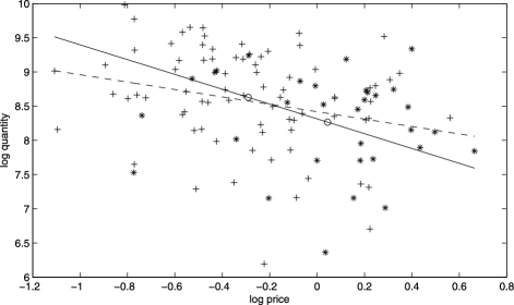
Figure 2: Scatterplot of log prices and log quantities by weather conditions.

For some purposes, the reduced-form or intention-to-treat effects may be of substantive interest. In the Fulton fish market example, people attempting to predict prices and quantities under the current regime may find these estimates of interest. They are of less interest to policy makers contemplating the introduction of a new tax. In simultaneous equations settings, the demand and supply functions are viewed as structural in the sense that they are not affected by interventions in the market such as new taxes. As such they, and not the reduced-form regression functions, are the key components of predictions of market outcomes under new regimes. This is somewhat different in many of the recent applications of instrumental variables methods in the statistics literature in the context of randomized experiments with noncompliance where the intention-to-treat effects are traditionally of primary interest.

Let me illustrate this with the Fulton Fish Market data collected by Graddy. For ease of illustration, let me simplify the instrument to a binary one: the weather conditions are good for catching fish ($Z_{t}=0$, fair weather, corresponding to low wind speed and low wave height) or stormy ($Z_{t}=1$, corresponding to relatively strong winds and high waves). The price is the average daily price in cents for one dealer, and the quantity is the daily quantity in pounds. The two estimated reduced forms are

$$\begin{array}[]{ccccc}\widehat{\ln Q}^{\mathrm{obs}}_{t}=&8.63&-&0.36&\times Z_{t}\\ &(0.08)&&(0.15)\end{array}$$

and

$$\begin{array}[]{ccccc}\widehat{\ln P}^{\mathrm{obs}}_{t}=&\!\!\!-0.29&+&0.34&\times Z_{t}.\\ &\!\!\!\hphantom{-}(0.04)&&(0.07)\end{array}$$

Hence, the instrumental variables estimate of the slope of the demand function is

$$\hat{\beta}^{d}=\frac{-0.36}{0.34}=-1.08\quad(\mbox{s.e. }0.46).$$

Another, perhaps more intuitive way of looking at these estimates is to consider the location of the average log quantity and average log price separately by weather conditions. Figure 2 presents the scatter plot of log quantity and log prices, with the stars indicating stormy days and the plus signs indicating calm days. On fair weather days the average log price is $-0.29$, and the average log quantity is 8.6. On stormy days, the average log price is 0.04, and the average log quantity is 8.3. These two loci are marked by circles in Figure 2. On stormy days, the price is higher and the quantity traded is lower than on fair weather days. This is used to estimate the slope of the demand function. The figure also includes the estimated demand function based on using the indicator for stormy days as an instrument for the price: the estimated demand function goes through the two points defined by the average of the log price and log quantity for stormy and fair weather days.

With the data collected by Graddy, it is more difficult to point identify the supply curve. The traditional route toward identifying the supply curve would rely on finding an instrument that shifts demand without directly affecting supply. Without such an instrument, we cannot point identify the effect of the introduction of the tax on quantity and prices. It is possible under weaker assumptions to find bounds on these estimands (e.g., Leamer (1981); Manski (2003)), but we do not pursue this here.

3.8 Recent Research on Simultaneous Equations Models

The traditional econometric literature on simultaneous equations models is surveyed in Hausman (1983). Compared to the discussion in the preceding sections, this literature focuses on a more general case, allowing for multiple endogenous variables and multiple instruments. The modern econometric literature, starting in the 1980s, has relaxed the linearity and additivity assumptions in specification (3) substantially. Key references to this literature are Brown (1983), Roehrig (1988), Newey and Powell (2003), Chesher (2003, 2010), Benkard and Berry (2006), Matzkin (2003, 2007), Altonji and Matzkin (2005), Imbens and Newey (2009), Hoderlein and Mammen (2007), Horowitz (2011) and Horowitz and Lee (2007). Matzkin (2007) provides a recent survey of this technically demanding literature. This literature has continued to use the observed outcome notation, making it more difficult to connect to the statistical literature. Here, I briefly review some of this literature. The starting point is a structural equation, in the potential outcome notation,

$$Y_{i}(x)=\alpha+\beta\cdot x+\varepsilon_{i}$$

and an instrument $Z_{i}$ that satisfies

$$Z_{i}\perp\varepsilon_{i}\quad\mbox{and}\quad Z_{i}\not\perp X_{i}.$$

The traditional econometric literature would formulate this in the observed outcome notation as

$$Y_{i}=\alpha+\beta\cdot X_{i}+\varepsilon_{i},\quad Z_{i}\perp\varepsilon_{i}\quad\mbox{and}\quad Z_{i}\not\perp X_{i}.$$

There are a number of generalizations considered in the modern literature. First, instead of assuming independence of the unobserved component and the instrument, part of the current literature assumes only that the conditional mean of the unobserved component given the instrument is free of dependence on the instrument, allowing the variance and other distributional aspects to depend on the value of the instrument; see Horowitz (2011). Another generalization of the linear model allows for general nonlinear function forms of the type

$$Y_{i}=g(X_{i})+\varepsilon_{i},\quad Z_{i}\perp\varepsilon_{i}\quad\mbox{and}\quad Z_{i}\not\perp X_{i},$$

where the focus is on nonparametric identification and estimation of $g(x)$; see Brown (1983), Roehrig (1988), Benkard and Berry (2006). Allowing for even more generality, researchers have studied nonadditive versions of these models with

$$Y_{i}=g(X_{i},\varepsilon_{i}),\quad Z_{i}\perp\varepsilon_{i}\quad\mbox{and}\quad Z_{i}\not\perp X_{i},$$

with $g(x,\varepsilon)$ strictly monotone in a scalar unobserved component $\varepsilon$. In these settings, point identification often requires strong assumptions on the support of the instrument and its relation to the endogenous regressor and, therefore, researchers have also explored bounds. See Matzkin (2003, 2007, 2008) and Imbens and Newey (2009).

4 A Modern Example: Randomized Experiments with Noncompliance and Heterogenous Treatment Effects

In this section, I will discuss part of the modern literature on instrumental variables methods that has evolved simultaneously in the statistics and econometrics literature. I will do so in the context of a second example. On the one hand, concern arose in the econometric literature about the restrictiveness of the functional form assumptions in the traditional instrumental variables methods and in particular with the constant treatment effect assumption that were commonly used in the so-called selection models (Heckman (1979); Heckman and Robb (1985)). The initial results in this literature demonstrated the difficulties in establishing point identification (Heckman (1990); Manski (1990)), leading to the bounds approach developed by Manski (1995, 2003). At the same time, statisticians analyzed the complications arising from noncompliance in randomized experiments (Robins (1989)) and the merits of encouragement designs (Zelen, 1979, 1990). By adopting a common framework and notation in Imbens and Angrist (1994) and Angrist, Imbens and Rubin (1996), these literatures have become closely connected and influenced each other substantially.

4.1 The McDonald, Hiu and Tierney (1992) Data

The canonical example in this literature is that of a randomized experiment with noncompliance. To illustrate the issues, I will use here data previously analyzed in Hirano et al. (2000) and McDonald, Hiu and Tierney (1992). McDonald, Hiu and Tierney (1992) carried out a randomized experiment to evaluate the effect of an influenza vaccination on flu-related hospital visits. Instead of randomly assigning individuals to receive the vaccination, the researchers randomly assigned physicians to receive letters reminding them of the upcoming flu season and encouraging them to vaccinate their patients. This is what Zelen (1979, 1990) refers to as an encouragement design. I discuss this using the potential outcome notation used for this particular set up in Angrist, Imbens and Rubin (1996), and in general sometimes referred to as the Rubin Causal Model (Holland (1986)), although there are important antecedents in Splawa-Neyman (1990). I consider two distinct treatments: the first the receipt of the letter, and second the receipt of the influenza vaccination. Let $Z_{i}\in\{0,1\}$ be the indicator for the receipt of the letter, and let $X_{i}\in\{0,1\}$ be the indicator for the receipt of the vaccination. We start by postulating the existence of four potential outcomes. Let $Y_{i}(z,x)$ be the potential outcome corresponding to the receipt of letter equal to $Z_{i}=z$, and the receipt of vaccination equal to $X_{i}=x$, for $z=0,1$ and $x=0,1$. In addition, we postulate the existence of two potential outcomes corresponding to the receipt of the vaccination as a function of the receipt of the letter, $X_{i}(z)$, for $z=0,1$. We observe for each unit in a population of size $N=2861$ the value of the assignment, $Z_{i}$, the treatment actually received, $X_{i}^{\mathrm{obs}}=X_{i}(Z_{i})$ and the potential outcome corresponding to the assignment and treatment received, $Y^{\mathrm{obs}}_{i}=Y_{i}(Z_{i},X_{i}(Z_{i}))$. Table 2 presents the number of individuals for each of the eight values of the triple $(Z_{i},X^{\mathrm{obs}}_{i},Y^{\mathrm{obs}}_{i})$ in the McDonald, Hiu and Tierney data set. It should be noted that the randomization in this experiment is at the physician level. I do not have physician indicators and, therefore, ignore the clustering. This will tend to lead to underestimation of the standard errors.

Table 2: Influenza data ($N=2861$)

Hospitalized for	Influenza
flu-related reasons	vaccine	Letter	Number of
$\bm{Y}_{\bolds{i}}^{\mathbf{obs}}$	$\bolds{X}^{\mathbf{obs}}_{\bolds{i}}$	$\bolds{Z}_{\bolds{i}}$	individuals
No	No	No	$1027$
No	No	Yes	$935$
No	Yes	No	$233$
No	Yes	Yes	$422$
Yes	No	No	$99$
Yes	No	Yes	$84$
Yes	Yes	No	$30$
Yes	Yes	Yes	$31$

4.2 Instrumental Variables Assumptions

There are four key of assumptions underlying instrumental variables methods beyond the no-interference assumption or SUTVA, with different versions for some of them. I will introduce these assumptions in this section, and in Section 5 discuss their substantive content in the context of some examples. The first assumption concerns the assignment to the instrument $Z_{i}$, in the flu example the receipt of the letter by the physician. The assumption requires that the instrument is as good as randomly assigned:

$$Z_{i}\perp\bigl{(}Y_{i}(0,0),Y_{i}(0,1),Y_{i}(1,0),$$ (11)

$$\hskip 48.0ptY_{i}(1,1),X_{i}(0),X_{i}(1)\bigr{)}$$

$$\eqntext{\mbox{(random assignment).}}$$ (12)

This assumption is often satisfied by design: if the assignment is physically randomized, as the letter in the flu example and as in many of the applications in the statistics literature (e.g., see the discussion in Robins (1989)), it is automatically satisfied. In other applications with observational data, common in the econometrics literature, this assumption is more controversial. It can in those cases be relaxed by requiring it to hold only within subpopulations defined by covariates $V_{i}$, assuming the assignment of the instrument is unconfounded:

$$Z_{i}\perp\bigl{(}Y_{i}(0,0),Y_{i}(0,1),Y_{i}(1,0),$$

$$\hskip 48.0ptY_{i}(1,1),X_{i}(0),X_{i}(1)\bigr{)}|V_{i}$$

$$\eqntext{(\mbox{unconfounded assignment given }V_{i}).}$$ (13)

This is identical to the generalization from random assignment to unconfounded assignment in observational studies. Either version of this assumption justifies the causal interpretation of Intention-To-Treat (ITT) effects, the comparison of outcomes by assignment to the treatment. In many cases, these ITT effects are only of limited interest, however, and this motivates the consideration of additional assumptions that do allow the researcher to make statements about the causal effects of the treatment of interest. It should be stressed, however, that in order to draw inferences beyond ITT effects, additional assumptions will be used; whether the resulting inferences are credible will depend on the credibility of these assumptions.

The second class of assumptions limits or rules out completely direct effects of the assignment (the receipt of the letter in the flu example) on the outcome, other than through the effect of the assignment on the receipt of the treatment of interest (the receipt of the vaccine). This is the most critical, and typically most controversial assumption underlying instrumental variables methods, sometimes viewed as the defining characteristic of instruments. One way of formulating this assumption is as

$$Y_{i}(0,x)=Y_{i}(1,x)\quad\mbox{for }x=0,1,\mbox{for all }i$$

$$\eqntext{\mbox{(exclusion restriction).}}$$ (14)

Robins (1989) formulates a similar assumption as requiring that the instrument is “not an independent causal risk factor” (Robins (1989), page 119). Under this assumption, we can drop the $z$ argument of the potential outcomes and write the potential outcomes without ambiguity as $Y_{i}(x)$. This assumption is typically a substantive one. In the flu example, one might be concerned that the physician, in response to the receipt of the letter, takes actions that affect the likelihood of the patient getting infected with the flu other than simply administering the flu vaccine. In randomized experiments with noncompliance, the exclusion restriction is sometimes made implicitly by indexing the potential outcomes only by the treatment $x$ and not the instrument $z$ (e.g., Zelen (1990)).

There are other, weaker versions of this assumption. Hirano et al. (2000) use a stochastic version of the exclusion restriction that only requires that the distribution of $Y_{i}(0,x)$ is the same as the distribution of $Y_{i}(1,x)$. Manski (1990) uses a weaker restriction that he calls a level set restriction, which requires that the average value of $Y_{i}(0,x)$ is equal to the average value of $Y_{i}(1,x)$. In another approach, Manski and Pepper (2000) consider monotonicity assumptions that restrict the sign of $Y_{i}(1,x)-Y_{i}(0,x)$ across individuals without requiring that the effects are completely absent.

Imbens and Angrist (1994) combine the random assignment assumption and the exclusion restriction by postulating the existence of a pair of potential outcomes $Y_{i}(x)$, for $x=0,1$, and directly assuming that

$$Z_{i}\perp\bigl{(}Y_{i}(0),Y_{i}(1)\bigr{)}.$$

A disadvantage of this formulation is that it becomes less clear exactly what role randomization of the instrument plays. Another version of this combination of the exclusion restriction and random assignment assumption does not require full independence, but assumes that the conditional mean of $Y_{i}(0)$ and $Y_{i}(1)$ given the instrument is free of dependence on the instrument. A concern with such assumptions is that they are functional form dependent: if they hold in levels, they do not hold in logarithms unless full independence holds.

A third assumption that is often used, labeled monotonicity by Imbens and Angrist (1994), requires that

$$X_{i}(1)\geq X_{i}(0)\quad\mbox{for all }i\quad\mbox{(monotonicity)},$$

for all units. This assumption rules out the presence of units who always do the opposite of their assignment [units with $X_{i}(0)=1$ and $X_{i}(1)=0$], and is therefore also referred to as the no-defiance assumption (Balke and Pearl (1995)). It is implicit in the latent index models often used in econometric evaluation models (e.g., Heckman and Robb, 1985). In the randomized experiments such as the flu example, this assumption is often plausible. There it requires that in response to the receipt of the letter by their physician, no patient is less likely to get the vaccine. Robins (1989) makes this assumption in the context of a randomized trial for the effect of AZT on AIDS, and describes the assumption as “often, but not always, reasonable” (Robins (1989), page 122).

Finally, we need the instrument to be correlated with the treatment, or the instrument to be relevant in the terminology of Phillips (1989) and Staiger and Stock (1997):

$$X_{i}\not\perp Z_{i}.$$

In practice, we need the correlation to be substantial in order to draw precise inferences. A recent literature on weak instruments is concerned with credible inference in settings where this correlation between the instrument and the treatment is weak; see Staiger and Stock (1997) and Andrews and Stock (2007).

The random assignment assumption and the exclusion restriction are conveniently captured by the graphical model below, although the monotonicity assumption does not fit in as easily. The unobserved component $U$ has a direct effect on both the treatment $X$ and the outcome $Y$ (captured by arrows from $U$ to $X$ and to $Y$). The instrument $Z$ is not related to the unobserved component $U$ (captured by the absence of a link between $U$ and $Z$), and is only related to the outcome $Y$ through the treatment $X$ (as captured by the arrow from $Z$ to $X$ and an arrow from $X$ to $Y$, and the absence of an arrow between $Z$ and $Y$).

I will primarily focus on the case with all four assumptions maintained, random assignment, the exclusion restriction, monotonicity and instrument relevance, without additional covariates, because this case has been the focus of, or a special case of the focus of, many studies, allowing me to compare different approaches. Methodological studies considering essentially this set of assumptions, sometimes without explicitly stating instrument relevance, and sometimes adding additional assumptions, include Robins (1989), Heckman (1990), Manski (1990), Imbens and Angrist (1994), Angrist, Imbens and Rubin (1996), Robins and Greenland (1996), Balke and Pearl (1995, 1997), Greenland (2000), Hernán and Robins (2006), Robins (1994), Robins and Rotnitzky (2004), Vansteelandt and Goetghebeur (2003), Vansteelandt et al. (2011), Hirano et al. (2000), Tan (2006, 2010), Abadie (2002, 2003), Duflo, Glennester and Kremer (2007), Brookhart et al. (2006), Martens et al. (2006), Morgan and Winship (2007), and others. Many more studies make the same assumptions in combination with a constant treatment effect assumption.

The modern literature analyzed this setting from a number of different approaches. Initially, the literature focused on the inability, under these four assumptions, to identify the average effect of the treatment. Some researchers, including prominently Manski (1990), Balke and Pearl (1995) and Robins (1989), showed that although one could not point-identify the average effect under these assumptions, there was information about the average effect in the data under these assumptions and they derived bounds for it. Another strand of the literature, starting with Imbens and Angrist (1994) and Angrist, Imbens and Rubin (1996) abandoned the effort to do inference for the overall average effect, and focused on subpopulations for which the average effect could be identified, the so-called compliers, leading to the local average treatment effect. We discuss the bounds approach in the next section (Section 4.3) and the local average treatment effect approach in Sections 4.4–4.6.

4.3 Point Identification versus Bounds

In a number of studies, the primary estimand is the average effect of the treatment, or the average effect for the treated:

$$\tau = \mathbb{E}\bigl{[}Y_{i}(1)-Y_{i}(0)\bigr{]}\quad\mbox{and}$$

$$\tau_{t} = \mathbb{E}\bigl{[}Y_{i}(1)-Y_{i}(0)|X_{i}=1\bigr{]}.$$

With only the four assumptions, random assignment, the exclusion restriction, monotonicity, and instrument relevance Robins (1989), Manski (1990) and Balke and Pearl (1995) established that the average treatment effect can often not be consistently estimated even in large samples. In other words, that it is often not point-identified.

Following this result, a number of different approaches have been taken. Heckman (1990) showed that if the instrument takes on values such that the probability of treatment given the instrument can be arbitrarily close to zero and one, then the average effect is identified. This is sometimes referred to as identification at infinity. Robins (1989) also formulates assumptions that allow for point identification, focusing on the average effect for the treated, $\tau_{t}$. These assumptions restrict the average value of the potential outcomes when not observed in terms of average outcomes that are observed. For example, Robins formulates the condition that

$$\mathbb{E}\bigl{[}Y_{i}(1)-Y_{i}(0)|Z_{i}=1,X_{i}=1\bigr{]}$$

$$\quad=\mathbb{E}\bigl{[}Y_{i}(1)-Y_{i}(0)|Z_{i}=0,X_{i}=1\bigr{]},$$

which, in combination with the random assignment and the exclusion restriction, this allows for point identification of the average effect for the treated. Robins also formulates two other assumptions, including one where the effects are proportional to survival rates $\mathbb{E}[Y_{i}(1)|Z_{i}=1,X_{i}=1]$ and $\mathbb{E}[Y_{i}(1)|Z_{i}=0,X_{i}=1]$ respectively, that also point-identifies the average effect for the treated. However, Robins questions the applicability of these results by commenting that “it would be hard to imagine that there is sufficient understanding of the biological mechanism$\ldots$ to have strong beliefs that any of the three conditions$\ldots$ is more likely to hold than either of the other two” (Robins (1989), page 122).

As an alternative to adding assumptions, Robins (1989), Manski (1990) and Balke and Pearl (1995), focused on the question what can be learned about $\tau$ or $\tau_{t}$ given these four assumptions that do not allow for point identification. Here, I focus on the case where the three assumptions, random assignment, the exclusion restriction and monotonicity are maintained (without necessarily instrument relevance holding), although Robins (1989) and Manski (1990) also consider other combinations of assumptions. For ease of exposition, I focus on the bounds for the average treatment effect $\tau$ under these assumptions, in the case where $Y_{i}(0)$ and $Y_{i}(1)$ are binary. Then

$$\mathbb{E}\bigl{[}Y_{i}(1)-Y_{i}(0)\bigr{]}$$

$$\quad\in\bigl{[}-\bigl{(}1-{\mathbb{E}}[X_{i}|Z_{i}=1]\bigr{)}\cdot\mathbb{E}[Y_{i}|Z_{i}=1,X_{i}=0]$$

$$\qquad\hskip 2.0pt{}+{\mathbb{E}}[Y_{i}|Z_{i}=1]-{\mathbb{E}}[Y_{i}|Z_{i}=0]$$

$$\qquad\hskip 2.0pt{}+{\mathbb{E}}[X_{i}|Z_{i}=0]\cdot\bigl{(}\mathbb{E}[Y_{i}|Z_{i}=0,X_{i}=1]-1\bigr{)},$$

$$\qquad\hskip 2.0pt\bigl{(}1-{\mathbb{E}}[X_{i}|Z_{i}=1]\bigr{)}$$

$$\qquad\hskip 2.0pt{}\cdot\bigl{(}1-\mathbb{E}[Y_{i}|Z_{i}=1,X_{i}=0]\bigr{)}$$

$$\qquad\hskip 2.0pt{}+{\mathbb{E}}[Y_{i}|Z_{i}=1]-{\mathbb{E}}[Y_{i}|Z_{i}=0]$$

$$\qquad\hskip 32.0pt{}+{\mathbb{E}}[X_{i}|Z_{i}=0]\cdot\mathbb{E}[Y_{i}|Z_{i}=0,X_{i}=1]\bigr{]},$$

which are known at the natural bounds. In this simple setting, this is a straightforward calculation. Work by Manski (1995, 2003, 2005, 2007), Robins (1989) and Hernán and Robins (2006) extends the partial identification approach to substantially more complex settings.

For the McDonald–Hiu–Tierney flu data, the estimated identified set for the population average treatment effect is

$$\mathbb{E}\bigl{[}Y_{i}(1)-Y_{i}(0)\bigr{]}\in[-0.24,0.64].$$

There is a growing literature developing methods for establishing confidence intervals for parameters in settings with partial identification taking sampling uncertainty into account; see Imbens and Manski (2004) and Chernozhukov, Hong and Tamer (2007).

4.4 Compliance Types

Imbens and Angrist (1994) and Angrist, Imbens and Rubin (1996) take a different approach. Rather than focusing on the average effect for the population that is not identified under the three assumptions given in Section 4.2, they focus on different average causal effects. A first key step in the Angrist–Imbens–Rubin set up is that we can think of four different compliance types defined by the pair of values of $(X_{i}(0),X_{i}(1))$, that is, defined by how individuals would respond to different assignments in terms of receipt of the treatment:

$$T_{i}=\cases{n\ (\mbox{never-taker})&$\mbox{if }X_{i}(0)=X_{i}(1)=0$,\cr c\ (\mbox{complier})&$\mbox{if }X_{i}(0)=0,X_{i}(1)=1$,\cr d\ (\mbox{defier})&$\mbox{if }X_{i}(0)=1,X_{i}(1)=0$,\cr a\ (\mbox{always-taker})&$\mbox{if }X_{i}(0)=X_{i}(1)=1$.}$$

Given the existence of deterministic potential outcomes this partitioning of the population into four subpopulations is simply a definition. It clarifies immediately that it will be difficult to identify the average effect of the primary treatment (the receipt of the vaccine) for the entire population: never-takers and always-takers can only be observed exposed to a single level of the treatment of interest, and thus for these groups any point estimates of the causal effect of the treatment must be based on extrapolation.

We cannot infer without additional assumptions the compliance type of any unit: for each unit we observe $X_{i}(Z_{i})$, but the data contain no information about the value of $X_{i}(1-Z_{i})$. For each unit, there are therefore two compliance types consistent with the observed behavior. We can also not identify the proportion of individuals of each compliance type without additional restrictions. The monotonicity assumption implies that there are no defiers. This, in combination with random assignment, implies that we can identify the population shares of the remaining three compliance types. The proportion of always-takers and never-takers are

$$\pi_{a} = \operatorname{pr}(T_{i}=a)=\operatorname{pr}(X_{i}=1|Z_{i}=0)\quad\mbox{and}$$

$$\pi_{n} = \operatorname{pr}(T_{i}=n)=\operatorname{pr}(X_{i}=0|Z_{i}=1),$$

respectively, and the proportion of compliers is the remainder:

$$\pi_{c}=\operatorname{pr}(T_{i}=c)=1-\pi_{a}-\pi_{n}.$$

For the McDonald–Hiu–Tierney data these shares are estimated to be

$$\hat{\pi}_{a}=0.189,\quad\hat{\pi}_{n}=0.692,\quad\hat{\pi}_{c}=0.119,$$

although, as I discuss in Section 5.2, these shares may not be consistent with the exclusion restriction.

4.5 Local Average Treatment Effects

If, in addition to monotonicity, we also assume that the exclusion restriction holds, Imbens and Angrist (1994) and Angrist, Imbens and Rubin (1996) show that the local average treatment effect or complier average causal effect is identified:

$$\tau_{\mathrm{late}} = \mathbb{E}\bigl{[}Y_{i}(1)-Y_{i}(0)|T_{i}=c\bigr{]}$$

$$= \frac{\mathbb{E}[Y_{i}|Z_{i}=1]-\mathbb{E}[Y_{i}|Z_{i}=0]}{\mathbb{E}[X_{i}|Z_{i}=1]-\mathbb{E}[X_{i}|Z_{i}=0]}.$$

The components of the right-hand side of this expression can be estimated consistently from a random sample $(Z_{i},X_{i},Y_{i})_{i=1}^{N}$. For the McDonald–Hiu–Tierney data, this leads to

$$\hat{\tau}_{\mathrm{late}}=-0.125\quad(\mbox{s.e. }0.090).$$

Note that just as in the supply and demand example, the causal estimand is the ratio of the intention-to-treat effects of the letter on hospitalization and of the letter on the receipt of the vaccine. These intention-to-treat effects are

$$\widehat{\mbox{ITT}}_{Y} = -0.015\quad(\mbox{s.e. }0.011),$$

$$\widehat{\mbox{ITT}}_{X} = \hat{\pi}_{c}=0.119\quad(\mbox{s.e. }0.016),$$

with the latter equal to the estimated proportion of compliers in the population.

Without the monotonicity assumption, but maintaining the random assignment assumption and the exclusion restriction, the ratio of ITT effects still has a clear interpretation. In that case, it is equal to a linear combination average of the effect of the treatment for compliers and defiers:

$$\frac{\mathbb{E}[Y_{i}|Z_{i}=1]-\mathbb{E}[Y_{i}|Z_{i}=0]}{\mathbb{E}[X_{i}|Z_{i}=1]-\mathbb{E}[X_{i}|Z_{i}=0]}$$

$$\quad=\frac{\operatorname{pr}(T_{i}=c)}{\operatorname{pr}(T_{i}=c)-\operatorname{pr}(T_{i}=d)}$$

$$\qquad{}\cdot\mathbb{E}\bigl{[}Y_{i}(1)-Y_{i}(0)|T_{i}=c\bigr{]}$$

$$\qquad{}-\frac{\operatorname{pr}(T_{i}=d)}{\operatorname{pr}(T_{i}=c)-\operatorname{pr}(T_{i}=d)}$$

$$\quad\qquad{}\cdot\mathbb{E}\bigl{[}Y_{i}(1)-Y_{i}(0)|T_{i}=d\bigr{]}.$$

This estimand has a clear interpretation if the treatment effect is constant across all units, but if there is heterogeneity in the treatment effects it is a weighted average with some weights negative. This representation shows that if the monotonicity assumption is violated, but the proportion of defiers is small relative to that of compliers, the interpretation of the instrumental variables estimand is not severely impacted.

4.6 Do We Care About the Local Average Treatment Effect?

The local average treatment effect is an unusual estimand. It is an average effect of the treatment for a subpopulation that cannot be identified in the sense that there are no units whom we know for sure to belong to this subpopulation, although there are some units whom we know do not belong to it. A more conventional approach is to start an analysis by clearly articulating the object of interest, say the average effect of a treatment for a well-defined population. There may be challenges in obtaining credible estimates of this object of interest, and along the way one may make more or less credible assumptions, but typically the focus remains squarely on the originally specified object of interest.

Here, the approach appears to be quite different. We started off by defining unit-level treatment effects for all units. We did not articulate explicitly what the target estimand was. In the McDonald–Hiu–Tierney influenza-vaccine application a natural estimand might be the population average effect of the vaccine. Then, apparently more or less by accident, the definition of the compliance types led us to focus on the average effects for compliers. In this example, the compliers were defined by the response in terms of the receipt of the vaccine to the receipt of the letter. It appears difficult to argue that this is a substantially interesting group, and in fact no attempt was made to do so.

This type of example has led distinguished researchers both in economics and in statistics to question whether and why one should care about the local average treatment effect. The economist Deaton writes “I find it hard to make any sense of the LATE [local average treatment effect]” (Deaton (2010), page 430). Pearl similarly wonders “Realizing that the population averaged treatment effect (ATE) is not identifiable in experiments marred by noncompliance, they have shifted attention to a specific response type (i.e., compliers) for which the causal effect was identifiable, and presented the latter [the local average treatment effect] as an approximation for ATE. $\ldots$ However, most authors in this category do not state explicitly whether their focus on a specific stratum is motivated by mathematical convenience, mathematical necessity (to achieve identification) or a genuine interest in the stratum under analysis” (Pearl (2011), page 3). Freedman writes “In many circumstances, the instrumental-variables estimator turns out to be estimating some data-dependent average of structural parameters, whose meaning would have to be elucidated” (Freedman (2006), pages 700–701). Let me attempt to clear up this confusion. See also Imbens (2010). An instrumental variables analysis is an analysis in a second-best setting. It would have been preferable if one had been able to carry out a well-designed randomized experiment. However, such an experiment was not carried out, and we have noncompliance. As a result, we cannot answer all the questions we might have wanted to ask. Specifically, if the noncompliance is substantial, we are limited in the questions we can answer credibly and precisely. Ultimately, there is only one subpopulation we can credibly (point-)identify the average effect of the treatment for, namely, the compliers.

It may be useful to draw an analogy. Suppose a researcher is interested in evaluating a medical treatment and suppose a randomized experiment had been carried out to estimate the average effect of this new treatment. However, the population of the randomized experiment included only men, and the researcher is interested in the average effect for the entire population, including both men and women. What should the researcher do? I would argue that the researcher should report the results for the men, and acknowledge the limitation of the results for the original question of interest. Similarly, in the instrumental variables I see the limitation of the results to the compliers as one that was unintended, but driven by the lack of identification for other subpopulations given the design of the study. This limitation should be acknowledged, but one should not drop the analysis simply because the original estimand cannot be identified. Note that our case with instrumental variables is slightly worse than in the gender example, because we cannot actually identify all individuals with certainty as compliers.

There are alternatives to this view. One approach is to focus solely or primarily on intention-to-treat effects. The strongest argument for that is in the context of randomized experiments with noncompliance. The causal interpretation of intention-to-treat effects is justified by the randomization. As Freedman writes, “Experimental data should therefore be analyzed first by comparing rates or averages, following the intention-to-treat principle. Such comparisons are justified because the treatment and control groups are balanced, within the limits of chance variation, by randomization” (Freedman (2006), page 701). Even in that case one may wish to also report estimates of the local average treatment effects because they may correspond more closely to the object of ultimate interest. The argument for focusing on intention-to-treat or reduced-form estimates is weaker in other settings. For example, in the Fulton Fish Market demand and supply application, the intention-to-treat effects are the effects of weather conditions on prices and quantities. These effects may be of little substantive interest to policy makers interested in tax policy. The substantive interest for these policy makers is almost exclusively in the structural effects of price changes on demand and supply, and reduced form effects are only of interest in sofar as they are informative about those structural effects. Of course, one should bear in mind that the reduced form or intention-to-treat effects rely on fewer assumptions.

A second alternative is associated with the partial identification approach by Manski (1990, 2002, 2003, 2007); see also Robins (1989) and Leamer (1981) for antecedents. In this setting that suggests maintaining the focus on the original estimand, say the overall average effect, we cannot estimate that accurately because we cannot estimate the average value of $Y_{i}(0)$ for always-takers or the average value of $Y_{i}(1)$ for nevertakers, but we can bound the average effect of interest because we know a priori that the average value of $Y_{i}(0)$ for always-takers and the average value of $Y_{i}(0)$ for nevertakers is restricted to lie in the unit interval. Manski’s is a principled and coherent approach. One concern with the approach is that it has often focused on reporting solely these bounds, leading researchers to miss relevant information that is available given the maintained assumptions. Two different data sets may lead to the same bounds even though in one case we may know that the average effect for one subpopulation (the compliers) is positive and statistically significantly different from zero whereas in the other case there need not be any evidence of a nonzero effect for any subpopulation. It would appear to be useful to distinguish between such cases by reporting estimates of both the local average treatment effect and the bounds.

5 The Substantive Content of the Instrumental Variables Assumptions

In this section, I will discuss the substantive content of the three key assumptions, random assignment, the exclusion restriction and the monotonicity assumption. I will not discuss here the fourth assumption, instrument relevance. In practice, the main issue with that assumption concerns the quality of inferences when the assumption is close to being violated. See Section 7.5 for more discussion, and Staiger and Stock (1997) for a detailed study.

5.1 Unconfoundedness of the Instrument

First, consider the random assignment or unconfoundedness assumption. In a slightly different setting, this is a very familiar assumption. Matching methods often rely on random assignment, either unconditionally or conditionally, for their justification.

In some of the leading applications of instrumental variables methods, this assumption is satisfied by design, when the instrument is physically randomized. For example, in the draft lottery example (Angrist, 1990), draft priority is used as an instrument for veteran status in an evaluation of the causal effect of veteran status on mortality and earnings. In that case, the instrument, the draft priority number was assigned by randomization. Similarly, in the flu example (Hirano et al., 2000), the instrument for influenza vaccinations, the letter to the physician, was randomly assigned.

In other cases, the conditional version of this assumption is more plausible. In the McClellan and Newhouse (1994) study, proximity of an individual to a hospital with particular facilities is used as an instrument for the receipt of intensive treatment of acute myocardial infarction. This proximity measure is not randomly assigned, and McClellan and Newhouse use covariates to make the unconfoundedness assumption more plausible. For example, they worry about differences between individuals living in rural versus urban areas. To adjust for such differences, they use as one of the covariates the distance to the nearest hospital (regardless of the facilities at the nearest hospital).

A key issue is that although on its own this random assignment or unconfoundedness assumption justifies a causal interpretation of the intention-to-treat effects, it is not sufficient for a causal interpretation of the instrumental variables estimand, the ratio of the ITT effects for outcome and treatment.

5.2 The Exclusion Restriction

Second, consider the exclusion restriction. This is the most critical and typically most controversial assumption underlying instrumental variables methods.

First of all, it has some testable implications; see Balke and Pearl (1997) and the recent discussions in Kitagawa (2009) and Ramsahai and Lauritzen (2011). This testable restriction can be seen most easily in a binary outcome setting. Under the three assumptions, random assignment, the exclusion restriction and monotonicity, the intention-to-treatment effect of the assignment on the outcome is the product of two causal effects. First, the average effect of the assignment on the outcome for compliers, and second, the intention-to-treat effect of the assignment on receipt of the treatment, which is equal to the population proportion of compliers. If the outcome is binary, the first factor is between $-1$ and 1. Hence, the intention-to-treat effect of the assignment on the outcome has to be bounded in absolute value by the intention-to-treat effect of the assignment on the receipt of the treatment. This is a testable restriction. If the outcomes are multivalued, there is in fact a range of restrictions implied by the assumptions. However, there exist no consistent tests that will reject the null hypothesis with probability going to one as the sample size increases in all scenarios where the null hypothesis is wrong.

Let us assess these restrictions in the flu example. Because

$$\operatorname{pr}(Y_{i}=1,X_{i}=0|Z_{i}=1)$$

$$\quad=\operatorname{pr}\bigl{(}Y_{i}(0)=1|T_{i}=n\bigr{)}\cdot\operatorname{pr}(T_{i}=n)$$

and

$$\operatorname{pr}(Y_{i}=1,X_{i}=0|Z_{i}=0)$$

$$\quad=\operatorname{pr}\bigl{(}Y_{i}(0)=1|T_{i}=n\mbox{ or }c\bigr{)}$$

$$\qquad{}\cdot\operatorname{pr}(T_{i}=n\mbox{ or }c)$$

$$\quad=\operatorname{pr}\bigl{(}Y_{i}(0)=1|T_{i}=n\bigr{)}\cdot\operatorname{pr}(T_{i}=n)$$

$$\qquad{}+\operatorname{pr}\bigl{(}Y_{i}(0)=1|T_{i}=c\bigr{)}\cdot\operatorname{pr}(T_{i}=c)$$

it follows that

$$\operatorname{pr}(Y_{i}=1,X_{i}=0|Z_{i}=1)$$

(18)

$$\quad\leq\operatorname{pr}(Y_{i}=1,X_{i}=0|Z_{i}=0).$$

There are three more restrictions in this setting with a binary outcome, binary treatment and binary instrument; see Imbens and Rubin (1997b), Balke and Pearl (1997) and Richardson, Evans and Robins (2011) for details. For the flu data, the simple frequency estimator for the left-hand side of (5.2) is $30/1389=0.0216$, and the right-hand side is $31/72=0.0211$, leading to a slight violation as pointed out in Richardson, Evans and Robins (2011) and Imbens and Rubin (2014). Although not statistically significant, it shows that these restrictions have content in practice.

To assess the plausibility of the exclusion restriction, it is often helpful to do so separately in subpopulations defined by compliance status. Let us first consider the exclusion restriction for always-takers, who would receive the influenza vaccine irrespective of the receipt of the letter by their physician. Presumably, such patients are generally at higher risk for the flu. Why would such patients be affected by a letter warning their physicians about the upcoming flu season when they will get inoculated irrespective of this warning? It may be that the letter led the physician to take other actions beyond giving the flu vaccine, such as encouraging the patient to avoid exposure. These other actions may affect health outcomes, in which case the exclusion restriction would be violated. The exclusion restriction for never-takers has different content. These patients would not receive the vaccine in any case. If their physicians did not regard the risk of flu as sufficiently high to encourage their patients to have the vaccination, presumably the physician would not take other actions either. For these patients, the exclusion restriction may therefore be reasonable.

Consider the draft lottery example. In that case, the always-takers are individuals who volunteer for military service irrespective of their draft priority number. It seems plausible that the draft priority number has no causal effect on their outcomes. never-takers are individuals who do not serve in the military irrespective of their draft priority number. If this is for medical reasons, or more generally reasons that make them ineligible to serve, this seems plausible. If, on the other hand these are individuals fit but unwilling to serve, they may have had to take actions to stay out of the military that could have affected their subsequent civilian labor market careers. Such actions may include extending their educational career, or temporarily leaving the country. Note that these issues are not addressed by the random assignment of the instrument.

In general, the concern is that the instrument creates incentives not only to receive the treatment, but also to take additional actions that may affect the outcome of interest. The nature of these actions may well differ by compliance type. Most important is to keep in mind that this assumption is typically a substantive assumption, not satisfied by design outside of double-blind, single-dose placebo control randomized experiments with noncompliance.

5.3 Monotonicity

Finally, consider the monotonicity or no-defiers assumption. Even though this assumption is often the least controversial of the three instrumental variables assumptions, it is still sometimes viewed with suspicion. For example, whereas Robins views the assumption as “often, but not always reasonable” (Robins (1989), page 122), Freedman (2006) wonders: “The identifying restriction for the instrumental-variables estimator is troublesome: just why are there no defiers?” (Freedman (2006), page 700). In many applications, it is perfectly clear why there should be no or at most few defiers. The instrument plays the role of an incentive for the individual to choose the active treatment by either making it more attractive to take the active treatment or less attractive to take the control treatment. As long as individuals do not respond perversely to this incentive, monotonicity is plausible with either no or a negligible proportion of defiers in the population. The term incentive is used broadly here: it may be a financial incentive, or the provision of information, or an imperfectly monitored legal requirement, but in all cases something that makes it more likely, at the individual level, that the individual participates in the treatment.

Let us consider some examples. If noncompliance is one-sided, and those assigned to the control group are effectively embargoed from receiving the treatment, monotonicity is automatically satisfied. In that case $X_{i}(0)=0$, and there are no always-takers or defiers. The example discussed in Sommer and Zeger (1991), Imbens and Rubin (1997a) and Greenland (2000) fits this set up.

In the flu application introduced in Section 4, the letter to the physician creates an additional incentive for the physician to provide the flu vaccine to a patient, something beyond any incentives the physician may have had already to provide the vaccine. Some individuals may already be committed to the vaccine, irrespective of the letter (the always-takers), and some may not be swayed by the receipt of the letter (the never-takers), and that is consistent with this assumption. Monotonicity only requires that there is no patient, who, if their physician receives the letter, would not take the vaccine, whereas they would have taken the vaccine in the absence of the letter.

Consider a second example, the influential draft lottery application by Angrist (1990) (see also Hearst, Newman and Hulley (1986)). Angrist is interested in evaluating the effect of military service on subsequent civilian earnings, using the draft priority established by the draft lottery as an instrument. Monotonicity requires that assigning an individual priority for the draft rather than not, may induce them to serve in the military, or may not affect them, but cannot induce them to switch from serving to not serving in the military. Again that seems plausible. Having high priority for the draft increases the cost of staying out of the military: that may not be enough to change behavior, but it would be unusual if the increased cost of staying out of the military induced an individual to switch from serving in the military to not serving.

As a third example, consider the Permutt and Hebel (1989) study of the effect of smoking on birthweight. Permutt and Hebel use the random assignment to a smoking-cessation program as an instrument for the amount of smoking. In this case, the monotonicity assumption requires that there are no individuals who as a causal effect of the assignment to the smoking-cessation program end up smoking more. There may be individuals who continue to smoke as much under either assignment and individuals who reduce smoking as a result of the assignment, but the assumption is that there is nobody who increases their smoking as a result of the smoking-cessation program. In all these examples, monotonicity requires individuals not to respond perversely to changes in incentives. Systematic and major violations in such settings seem unlikely.

In other settings, the assumption is less attractive. Suppose a program has assignment criteria that are checked by two administrators. Individuals entering the assignment process are assigned randomly to one of the two administrators. The assignment criteria may be interpreted slightly differently by the two administrators, with on average administrator A being more strict than administrator B. Monotonicity requires that anyone admitted by administrator A would also be admitted by administrator B, or vice-versa. In this type of setting, monotonicity does not appear to be as plausible as it is in the settings where the instrument can be viewed as creating an incentive to participate in the treatment. For example, in an analysis of the effect of prison time on recidivism, Aizer and Doyle (2013) use random assignment of cases to judges, and in an analysis of the effect of bankruptcy, Dobbie and Song (2013) use random assignment of bankruptcy applications to judges.

The discussion in this section focuses primarily on the case with a binary treatment and a binary instrument. In cases with multivalued treatments, the monotonicity can be generalized in two different ways. In both cases, it may be less plausible than in the binary case. Let $X_{i}(z)$ be the potential treatment level associated with the assignment $z$. One can generalize the monotonicity assumption for the binary instrument case to this case as

$$X_{i}(z)\mbox{ is nondecreasing in }z\quad\mbox{for all }i$$

$$\eqntext{\mbox{(monotonicity in instrument)}.}$$ (19)

This generalization is used in Angrist and Imbens (1995). It is consistent with the view of the instrument as changing the incentive to participate in the treatment: increasing the incentive cannot decrease the level of the treatment received. Angrist and Imbens show that this assumption has testable implications.

An alternative generalization is

$$\mbox{if }X_{i}(z)>X_{j}(z)\quad$$

$$\quad\mbox{then }X_{i}\bigl{(}z^{\prime}\bigr{)}\geq X_{j}\bigl{(}z^{\prime}\bigr{)}\quad\mbox{for all }z,z^{\prime},i,j$$

$$\eqntext{\mbox{(monotonicity in unobservables).}}$$ (20)

This assumption, referred to as rank preservation in Robins (1986), implicitly ranks all units in terms of some unobservables (Imbens (2007)). It assumes this ranking is invariant to the level of the instrument. It implies that if $X_{i}(z)>X_{j}(z)$, then it cannot be that $X_{j}(z^{\prime})>X_{i}(z^{\prime})$. It is equivalent to the “continuous prescribing preference” in Hernán and Robins (2006).

In both cases, the special case with a binary treatment is identical to the previously stated monotonicity. In settings with multivalued treatments, these assumptions are more restrictive than in the binary treatment case. In the demand and supply example in Section 3 with linear supply and demand functions, both the monotonicity in the instrument and monotonicity in the unobservables conditions are satisfied.

6 The Link to the Textbook Discussions of Instrumental Variables

Most textbook discussions of instrumental variables use a framework that is quite different at first sight from the potential outcome set up used in Sections 4 and 5. These textbook discussions (graduate texts include Wooldridge, 2010; Angrist and Pischke (2009); Greene (2011); and Hayashi (2000), and introductory undergraduate textbooks include Wooldridge (2008); and Stock and Watson (2010)) are often closer to the simultaneous equations example from Section 3. An exception is Manski (2007) who uses the potential outcome set up used in this discussion. In this section I will discuss the standard textbook set up and relate it to the potential outcome framework and the simultaneous equations set up.

The textbook version of instrumental variables does not explicitly define the potential outcomes. Instead the starting point is a linear regression function describing the relation between the realized (observed) outcome $Y_{i}$, the endogenous regressor of interest $X_{i}$ and other regressors $V_{i}$:

$$Y^{\mathrm{obs}}_{i}=\beta_{0}+\beta_{1}X_{i}+\beta_{2}^{\prime}V_{i}+\varepsilon_{i}.$$ (21)

These other regressors a well as the instruments are often referred to in the econometric literature as exogenous variables. Although this term does not have a well-defined meaning, informally it includes variables that Cox (1992) called attributes, as well as potential causes whose assignment is unconfounded. This set up covers both the demand function setting and the randomized experiment example. Although this equation looks like a standard regression function, that similarity is misleading. Equation (21) is not an ordinary regression function in the sense that the first part does not represent the conditional expectation of the outcome $Y_{i}$ given the right-hand side variables $X_{i}$ and $V_{i}$. Instead it is what is sometimes called a structural equation representing the causal response to changes in the input $X_{i}$.

The key assumption in this formulation is that the unobserved component $\varepsilon_{i}$ in this regression function is independent of the exogenous regressors $V_{i}$ and the instruments $Z_{i}$, or, formally

$$\varepsilon_{i}\perp(Z_{i},V_{i}).$$ (22)

The unobserved component is not independent of the endogenous regressor $X_{i}$ though. The value of the regressor $X_{i}$ may be partly chosen by individual $i$ to optimize some objection function as in the noncompliance example, or the result of an equilibrium condition as in the supply and demand model. The precise relation between $X_{i}$ and $\varepsilon_{i}$ is often not fully specified.

How does this set up relate to the earlier discussion involving potential outcomes? Implicitly, there is in the background of this set up a causal, unit-level response function. In the potential outcome notation, let $Y_{i}(x)$ denote this causal response function for unit $i$, describing for each value of $x$ the potential outcome corresponding to that level of the treatment for that unit. Suppose the conditional expectation of this causal response function is linear in $x$ and some exogenous covariates:

$$\mathbb{E}\bigl{[}Y_{i}(x)|V_{i}\bigr{]}=\beta_{0}+\beta_{1}\cdot x+\beta_{2}^{\prime}V_{i}.$$ (23)

Moreover, let us make the (strong) assumption that the difference between the response function $Y_{i}(x)$ and its conditional expectation does not depend on $x$, so we can define the residual unambiguously as

$$\varepsilon_{i}=Y_{i}(x)-\bigl{(}\beta_{0}+\beta_{1}\cdot x+\beta_{2}^{\prime}V_{i}\bigr{)},$$

with the equality holding for all $x$. The residual $\varepsilon_{i}$ is now uncorrelated with $V_{i}$ by definition. We will assume that it is in fact independent of $V_{i}$. Now suppose we have an instrument $Z_{i}$ such that

$$Y_{i}(x)\perp Z_{i}|V_{i}.$$

This assumption is, given the linear representation for $Y_{i}(x)$, equivalent to

$$\varepsilon_{i}\perp Z_{i}|V_{i}.$$

In combination with the assumption that $\varepsilon_{i}\perp V_{i}$, this gives us the textbook version of the assumption given in (22). We observe $V_{i}$, $X_{i}$, the instrument $Z_{i}$, and the realized outcome

$$Y^{\mathrm{obs}}_{i}=Y_{i}(X_{i})=\beta_{0}+\beta_{1}X_{i}+\beta_{2}^{\prime}V_{i}+\varepsilon_{i},$$

which is the starting point in the econometric textbook discussion (21).

This set up is more restrictive than it needs to be. For example, the assumption that the difference between the response function $Y_{i}(x)$ and its conditional expectation does not depend on $x$ can be relaxed to allow for variation in the slope coefficient,

$$Y_{i}(x)-Y_{i}(0)=\beta_{1}\cdot x+\eta_{i}\cdot x,$$

as long as the $\eta_{i}$ satisfies conditions similar to those on $\varepsilon_{i}$. The modern literature (e.g., Matzkin (2007)) discusses such models in more detail.

One key feature of the textbook version is that there is no separate role for the monotonicity assumption. Because the linear model implicitly assumes that the per-unit causal effect is constant across units and levels of the treatment, violations of the monotonicity assumption do not affect the interpretation of the estimand. A second feature of the textbook version is that the exclusion restriction and the random assignment assumption are combined in (22). Implicitly, the exclusion restriction is captured by the absence of $Z_{i}$ in the equation (21), and the (conditional) random assignment is captured by (22).

7 Extensions and Generalizations

In this section, I will briefly review some of other approaches taken in the instrumental variables literature. Some of these originate in the statistics literature, some in the econometrics literature. They reflect different concerns with the traditional instrumental variables methods, sometimes because of different applications, sometimes because of different traditions in econometrics and statistics. This discussion is not exhaustive. I will focus on highlighting the most interesting developments and provide some references to the relevant literature.

7.1 Model-based Approaches to Estimation and Inference

Traditionally, instrumental variables analyses relied on linear regression methods. Additional explanatory variables are incorporated linearly in the regression function. The recent work in the statistics literature has explored more flexible approaches to include covariates. These approaches often involve modeling the conditional distribution of the endogenous regressor given the instruments and the exogenous variables. This is in contrast to the traditional econometric literature which has focused on settings and methods that do not rely on such models.

Robins (1989, 1994), Hernán and Robins (2006), Greenland (2000), Robins and Rotnitzky (2004) and Tan (2010) developed an approach that allow for identification of average treatment effect by adding parametric modelling assumptions. This approach starts with the specification of what they call the structural mean, the expectation of $Y_{i}(x)$. This structural mean can be the conditional mean given covariates, or the marginal mean, labeled the marginal structural mean. The specification for this expectation is typically parametric. Then estimating equations for the parameters of these models are developed. In the simple setting considered here, this would typically lead to the same estimators considered already. An important virtue of the method is that it has been extended to much more general settings, in particular with time-varying covariates and dynamic treatment regimes in a series of papers. In other settings, it has also led to the development of doubly robust estimators (Robins and Rotnitzky (2004)). A key feature of the models is that the models are robust in a particular sense. Specifically, the estimators for the average treatment effects are consistent irrespective of the misspecification of the model, in the absence of intention-to-treat effects (what they call the conditional ITT null).

Imbens and Rubin (1997a) and Hirano et al. (2000) propose building a parametric model for the compliance status in terms of additional covariates, combined with models for the potential outcomes conditional on compliance status and covariates. Given the monotonicity assumption, there are three compliance types: never-takers, always-takers and compliers. A natural model for compliance status given individual characteristics $V_{i}$ is therefore a trinomial logit model:

$$\operatorname{pr}(T_{i}=n|V_{i}=v) = \frac{\exp(v^{\prime}\gamma_{n})}{1+\exp(v^{\prime}\gamma_{n})+\exp(v^{\prime}\gamma_{n})},$$

$$\operatorname{pr}(T_{i}=a|V_{i}=v) = \frac{\exp(v^{\prime}\gamma_{a})}{1+\exp(v^{\prime}\gamma_{n})+\exp(v^{\prime}\gamma_{n})}$$

and

$$\operatorname{pr}(T_{i}=c|V_{i}=v)=\frac{1}{1+\exp(v^{\prime}\gamma_{n})+\exp(v^{\prime}\gamma_{n})}.$$

With continuous outcomes, the conditional outcome distributions given compliance status and covariates may be normal:

$$Y_{i}(x)|T_{i}=t,\quad V_{i}=v\sim\mathcal{N}\bigl{(}\beta_{tx}^{\prime}v,\sigma^{2}_{tx}\bigr{)},$$

for $(t,x)=(n,0),(a,1),(c,0),(c,1)$. With binary outcomes, one may wish to use logistic regression models here. This specification defines the likelihood function. Hirano et al. (2000) apply this to the flu data discussed before. Simulations in Richardson, Evans and Robins (2011) suggest that the modeling of the compliance status here is key. Specifically, they point out that even in the absence of ITT effects there can be biases if the model of the compliance status is misspecified.

Like Hirano et al. (2000), Richardson, Evans and Robins (2011) build parametric model only for the identified distributions. They use them to estimate the bounds so that the parametric assumptions do not contain identifying information.

Little and Yau (1998) and Yau and Little (2001) similarly model the conditional expectation of the outcome given compliance status and covariates. In their application, there are no always-takers, only never-takers and compliers. Their specification specifies parametric forms for the conditional means given the compliance types and the treatment status:

$$\mathbb{E}\bigl{[}Y_{i}(0)|T_{i}=n,V_{i}=v\bigr{]} = \beta_{n0}+\beta_{n1}^{\prime}v,$$

$$\mathbb{E}\bigl{[}Y_{i}(0)|T_{i}=c,V_{i}=v\bigr{]} = \beta_{c00}+\beta_{c01}^{\prime}v$$

and

$$\mathbb{E}\bigl{[}Y_{i}(1)|T_{i}=c,V_{i}=v\bigr{]}=\beta_{c00}+\beta_{c11}^{\prime}v.$$

7.2 Principal Stratification

Frangakis and Rubin (2002) generalize the latent compliance type approach to instrumental variables in an important and novel way. Their focus is on the causal effect of a binary treatment on some outcome. However, it is not the average effect of the treatment they are interested in, but the average within a subpopulation. It is the way this subpopulation is defined that creates the complications as well as the connection to instrumental variables. There is a post-treatment variable that may be affected by the treatment. Frangakis and Rubin postulate the existence of a pair of potential outcomes for this post-treatment variable. The subpopulation of interest is then defined by the values for the pair of potential outcomes for this post-treatment variables.

Let us consider two examples: first, the randomized experiment with noncompliance. The treatment here is the random assignment. The post-treatment variable is the actual receipt of the treatment. The pair of potential outcomes for this post-treatment variable captures the compliance status. The subpopulation of interest is the subpopulation of compliers.

The second example shows how principal stratification generalizes the instrumental variables set up to other cases. Examples of this type are considered in Zhang, Rubin and Mealli (2009), Frumento et al. (2012) and Robins (1986). Suppose we have a randomized experiment with perfect compliance. The primary outcome is survival after one year. For patients who survive, a quality of life measure is observed. We may be interested in the effect of the treatment on quality of life. This is only defined for patients who survive up to one year. The principal stratification approach suggests focusing on the subpopulation or principal stratum of patients who survive irrespective of the treatment assignment. Membership in this stratum is not observed, and so we cannot directly estimate the average effect of the treatment on quality of life for individuals in this stratum, but the data are generally still informative about such effects, particularly under monotonicity assumptions.

7.3 Randomization Inference with Instrumental Variables

Most of the work on inference in instrumental variables settings is model-based. After specifying a model relating the treatment to the outcome, the conditional distribution or conditional mean of outcomes given instruments is derived. The resulting inferences are conditional on the values of the instruments. A very different approach is taken in Rosenbaum (1996) and Imbens and Rosenbaum (2005).

Rosenbaum focuses on the distribution for statistics generated by the random assignment of the instruments. In the spirit of the work by Fisher (1925) confidence intervals for the parameter of interest, $\beta_{1}$ in equation (23) are based on this randomization distribution. Similar to confidence intervals for treatment effects based on inverting conventional Fisher $p$-values, these intervals have exact coverage under the stated assumptions. However, these results rely on arguably restrictive constant treatment effect assumptions.

7.4 Matching and Instrumental Variables

In many observational studies using instrumental variables approaches, the instruments are not randomly assigned. In that case, adjustment for additional pretreatment variables can sometimes make causal inferences more credible. Even if the instrument is randomly assigned, such adjustments can make the inferences more precise. Traditionally, in econometrics these adjustments are based on regression methods. Recently, in the statistics literature matching methods have been proposed as a way to do the adjustment for pretreatment variables (Baiocchi et al., 2010).

7.5 Weak Instruments

One concern that has arisen in the econometrics literature is about weak instruments. For an instrument to be helpful in estimating the effect of the treatment, it not only needs to have no direct effect on the outcome, it also needs to be correlated with the treatment. Suppose this correlation is very close to zero. In the simple case, the IV estimator is the ratio of covariances,

$$\hat{\beta}_{1,\mathrm{iv}} = \frac{\widehat{\operatorname{cov}}(Y_{i},Z_{i})}{\widehat{\operatorname{cov}}(X_{i},Z_{i})}$$

$$= \frac{({1}/{N})\sum_{i=1}^{N}(Y_{i}-\overline{Y})(Z_{i}-\overline{Z})}{({1}/{N})\sum_{i=1}^{N}(X_{i}-\overline{X})(Z_{i}-\overline{Z})}.$$

The distribution of this ratio can be approximated by a normal distribution in large samples, as long as the covariance in the denominator is nonzero in the population. If the population value of the covariance in the denominator is exactly zero, the distribution of the ratio $\hat{\beta}_{1,\mathrm{iv}}$ is Cauchy in large samples, rather than normal (Phillips (1989); Staiger and Stock (1997)). The weak instrument literature is concerned with the construction of confidence intervals in the case the covariance is close to zero. Interest in this problem rose sharply after a study by Angrist and Krueger (1991), which remains the primary empirical motivation for this literature. Angrist and Krueger were interested in estimating the causal effect of years of education on earnings. They exploited variation in educational achievement by quarter of birth attributed to differences in compulsory schooling laws. These differences in average years of education by quarter of birth were small, and they attempted to improve precision of their estimators by including interactions of the basic instruments, the three quarter of birth dummies, with indicators for year and state of birth. Bound, Jaeger and Baker (1995) showed that the estimates using the interactions as additional instruments were potentially severely affected by the weakness of the instruments. In one striking analysis, they reestimated the Angrist–Krueger regressions using randomly generated quarter of birth data (uncorrelated with earnings or years of education). One might have expected, and hoped, that in that case one would find an imprecisely estimated effect. Surprisingly, Bound, Jaeger and Baker (1995) found that the confidence intervals constructed by Angrist and Krueger suggested precisely estimated effects for the effect of years of education on earnings. It was subsequently found that with weak instruments the TSLS estimator, especially with many instruments, was biased, and that the standard variance estimator led to confidence intervals with substantial undercoverage (Bound, Jaeger and Baker (1995); Staiger and Stock (1997); Chamberlain and Imbens (2004)).

Motivated by the Bound–Jaeger–Baker findings, the weak and many instruments literature focused on point and interval estimators with better properties in settings with weak instruments. Starting with Staiger and Stock (1997), a literature developed to construct confidence intervals for the instrumental variables estimand that remained valid irrespective of the strength of the instruments. A key insight was that confidence intervals based on the inversion of Anderson–Rubin (1949) statistics have good properties in settings with weak instruments; see also Moreira (2003), Andrews and Stock (2007), Kleibergen (2002) and Andrews, Moreira and Stock (2006).

Let us look at the simplest case with a single endogenous regressor, a single instrument, and no additional regressors and normally distributed residuals:

$$Y_{i}(x)=\beta_{0}+\beta_{1}\cdot x+\varepsilon_{i}\quad\mbox{with }\varepsilon_{i}|Z_{i}\sim\mathcal{N}\bigl{(}0,\sigma^{2}_{\varepsilon}\bigr{)}.$$

The Anderson–Rubin statistic is, for a given value of $b$

$$\operatorname{AR}(b) = \Biggl{(}\frac{1}{\sqrt{N}}\sum_{i=1}^{N}(Z_{i}-\overline{Z})\cdot(Y_{i}-b\cdot X_{i})\Biggr{)}^{2}$$

$${}\bigg{/}\Biggl{(}\frac{1}{N}\sum_{i=1}^{N}(Z_{i}-\overline{Z})^{2}\cdot\hat{\sigma}^{2}_{\varepsilon}\Biggr{)},$$

where $\overline{Z}=\sum_{i=1}^{N}Z_{i}/N$, and for some estimate of the residual variance $\sigma^{2}_{\varepsilon}$. At the true value $b=\beta_{1}$, the AR statistic has in large samples a chi-squared distribution with one degree of freedom. Staiger and Stock (1997) propose constructing a confidence interval by inverting this test statistic:

$$\mathrm{CI}^{0.95}(\beta_{1})=\bigl{\{}b|\operatorname{AR}(b)\leq 3.84\bigr{\}}.$$

The subsequent literature has extended this by allowing for multiple instruments and developed various alternatives, all with the focus on methods that remain valid irrespective of the strength of the instruments; see Andrews and Stock (2007) for an overview of this literature.

7.6 Many Instruments

Another strand of the literature motivated by the Angrist–Krueger study focused on settings with many weak instruments. The concern centered on the Bound, Jaeger and Baker (1995) finding that in a setting similar to the Angrist–Krueger setting using TSLS with many randomly generated instruments led to confidence intervals that had very low coverage rates.

To analyze this setting, Bekker (1994) considered the behavior of various estimators under an asymptotic sequence where the number of instruments increases with the sample size. Asymptotic approximations to sampling distributions based on this sequence turned out to be much more accurate than those based on conventional asymptotic approximations. A key finding in Bekker (1994) is that under such sequences one of the leading estimators, Two-Stage-Least-Squares (TSLS, see the Appendix for details) estimator is no longer consistent, whereas another estimator, Limited Information Maximum Likelihood (LIML, again see the Appendix for details) estimator remains consistent although the variance under this asymptotic sequence differs from that under the standard sequence; see also Kunitomo (1980), Morimune (1983), Bekker and van der Ploeg (2005), Chamberlain and Imbens (2004), Chao and Swanson (2005), Hahn (2002), Hansen, Hausman and Newey (2008), Kolesár et al. (2013).

7.7 Proxies for Instruments

Hernán and Robins (2006) and Chalak (2011) explores settings where the instrument is not directly observed. Instead a proxy variable $Z^{*}_{i}$ is observed. This proxy variable is correlated with the underlying instrument $Z_{i}$, but not perfectly so. The potential outcomes $Y_{i}(z,x)$ are still defined in terms of the underlying, unobserved instrument $Z_{i}$. The unobserved instrument $Z_{i}$ satisfies the instrumental variables assumptions, random assignment, the exclusion restriction and the monotonicity assumption. In addition, the observed proxy $Z_{i}^{*}$ satisfies

$$Z_{i}^{*} \perp Y_{i}(0,0),Y_{i}(0,1),Y_{i}(1,0),$$

$${}Y_{i}(1,1),X_{i}(0),X_{i}(1)|Z_{i}.$$

Chalak shows that the ratio of covariances (now no longer the ratio of intention-to-treat effects) still has an interpretation of an average causal effect.

7.8 Regression Discontinuity Designs

Regression Discontinuity (RD) designs attempt to estimate causal effects of a binary treatment in settings where the assignment mechanism is a deterministic function of a pretreatment variable. In the sharp version of the RD design, the assignment mechanism takes the form

$$X_{i}=\mathbf{1}_{V_{i}\geq c},$$

for some fixed threshold $c$: all units with a value for the covariate $V_{i}$ exceeding $c$ receive the treatment and all units with a value for $V_{i}$ less than $c$ are in the control group. Under smoothness assumptions, it is possible in such settings to estimate the average effect of the treatment for units with a value for the pretreatment variable equal to $V_{i}\approx c$:

$$\mathbb{E}\bigl{[}Y_{i}(1)-Y_{i}(0)|V_{i}=c\bigr{]}$$

$$\quad=\lim_{w\uparrow c}\mathbb{E}[Y_{i}|V_{i}=w]-\lim_{w\downarrow c}\mathbb{E}[Y_{i}|V_{i}=w].$$

These designs were introduced by Thistlewaite and Campbell (1960), and have been used in psychology, sociology, political science and economics. For example, many educational programs have eligibility criteria that allow for the application of RD methods; see Cook (2008) for a recent historical perspective and Imbens and Wooldridge (2009) for a recent review.

A generalization of the sharp RD design is the Fuzzy Regression Discontinuity or FRD design. In this case, the probability of receipt of the treatment increases discontinuously at the threshold, but not necessarily from zero to one:

$$\lim_{w\downarrow c}\operatorname{pr}(X_{i}=1|V_{i}=w)\neq\lim_{w\uparrow c}\operatorname{pr}(X_{i}=1|V_{i}=w).$$

In that case, it is no longer possible to consistently estimate the average effect of the treatment for all units at the threshold. Hahn, Todd and Van der Klaauw (2001) demonstrate that there is a close link to the instrumental variables set up. Specifically Hahn, Todd and Van der Klaauw show that one can estimate a local average treatment effect at the threshold. To be precise, one can identify the average effect of the treatment for those who are on the margin of getting the treatment:

$$\mathbb{E}\Bigl{[}Y_{i}(1)-Y_{i}(0)\big{|}$$

$$\quad\hskip 2.0pt{}V_{i}=c,\lim_{w\uparrow c}X_{i}(w)=0,\lim_{w\downarrow c}X_{i}(w)=1\Bigr{]}$$

$$\quad=\frac{\lim_{w\uparrow c}\mathbb{E}[Y_{i}|V_{i}=w]-\lim_{w\downarrow c}\mathbb{E}[Y_{i}|V_{i}=w]}{\lim_{w\uparrow c}\mathbb{E}[X_{i}|V_{i}=w]-\lim_{w\downarrow c}\mathbb{E}[X_{i}|V_{i}=w]}.$$

This estimand can be estimated as the ratio of an estimator for the discontinuity in the regression function for the outcome and an estimator for the discontinuity in the regression function for the treatment of interest.

8 Conclusion

In this paper, I review the connection between the recent statistics literature on instrumental variables and the older econometrics literature. Although the econometric literature on instrumental variables goes back to the 1920s, until recently it had not made much of an impact on the statistics literature. The recent statistics literature has combined some of the older insights from the econometrics instrumental variables literature with the separate literature on causality, enriching both in the process.

Appendix: Estimation and Inference, Two-Stage-Least-Squares and Other Traditional Methods

.1 Set up

In this section, I will discuss the traditional econometric approaches to estimation and inference in instrumental variables settings. Part of the aim of this section is to provide easier access to the econometric literature and terminology on instrumental variables, and to provide a perspective and context for the recent advances.

The textbook setting is the one discussed in the previous section, where a scalar outcome $Y_{i}$ is linearly related to a scalar covariate of interest $X_{i}$. In addition, there may be additional exogenous covariates $V_{i}$. The traditional model is

$$Y_{i}=\beta_{0}+\beta_{1}X_{i}+\beta_{2}^{\prime}V_{i}+\varepsilon_{i}.$$ (24)

In addition, we have a vector of instrumental variables $Z_{i}$, with dimension $K$.

An important distinction in the traditional econometric literature is between the case with a single instrument ($K=1$), and the case with more than one instrument ($K>1$). More generally, with more than one endogenous regressor, the distinction is between the case with the number of instruments equal to the number of endogenous regressors and the case with the number of instruments larger than the number of endogenous regressors. In the empirical literature, there are few credible examples with more than one endogenous regressor, so I focus here on the case with a single endogenous regressor. The first case, with a single instrument, is referred to as the just-identified case, and the second, with multiple instruments and a single endogenous regressor, as the over-identified case. In the textbook setting with a linear model and constant coefficients, this distinction has motivated different estimators and specification tests. In the modern literature, with its explicit allowance for heterogeneity in the treatment effects, these tests, and the distinction between the various estimators, are of less interest. In the recent statistics literature, little attention has been paid to the over-identified case with multiple instruments. An exception is Small (2007).

Obviously, it is often difficult in applications to find even a single variable that satisfies the conditions for it to be a valid instrument. This raises the question how relevant the literature focusing on methods to deal with multiple instruments is for empirical practice. There are two classes of applications where multiple instruments could credible arise. First, suppose one has a single continuous (or multivalued) instrument that satisfies the instrumental variables assumptions, monotonicity, random assignment and the exclusion restriction. Then any monotone function of the instruments also satisfies these assumptions, and one can use multiple monotone functions of the original instrument as instruments. Second, if one has a single instrument in combination with exogenous covariates, then one can use interactions of the instrument and the covariates to generate additional instruments.

Consider, for example, the Fulton fish market study by Graddy (1995, 1996). Graddy uses weather conditions as an instrument that affects supply but not demand. Specifically, she measures wind speed and wave height, giving her two basic instruments. She also constructs functions of these basic instruments, such as indicators that the wind speed or wave height exceeds some threshold.

.2 The Just-Identified Case with no Additional Covariates

The traditional approach to estimation in this case is to use what is known in the econometrics literature as the instrumental variables estimator. In the case without additional exogenous covariates, the most widely used estimator is simply the ratio of two covariances:

$$\hat{\beta}_{1,\mathrm{iv}} = \frac{\widehat{\operatorname{cov}}(Y_{i},Z_{i})}{\widehat{\operatorname{cov}}(X_{i},Z_{i})}$$

$$= \frac{({1}/{N})\sum_{i=1}^{N}(Y_{i}-\overline{Y})(Z_{i}-\overline{Z})}{({1}/{N})\sum_{i=1}^{N}(X_{i}-\overline{X})(Z_{i}-\overline{Z})},$$

where $\overline{Y}$, $\overline{Z}$ and $\overline{X}$ denote sample averages. If the instrument $Z_{i}$ is binary, this is also known as the Wald estimator:

$$\hat{\beta}_{1,\mathrm{iv}}=\frac{\overline{Y}_{1}-\overline{Y}_{0}}{\overline{X}_{1}-\overline{X}_{0}},$$

where for $z=0,1$

$$\overline{Y}_{z}=\frac{1}{N_{z}}\sum_{i:Z_{i}=z}Y_{i},\quad\overline{X}_{z}=\frac{1}{N_{z}}\sum_{i:Z_{i}=z}X_{i},$$

and $N_{1}=\sum_{i=1}^{N}Z_{i}$ and $N_{0}=\sum_{i=1}^{N}(1-Z_{i})$.

One can interpret this estimator in two different ways. These interpretations are useful for motivating extensions to settings with multiple instruments and additional exogenous regressors. First, the indirect least squares interpretation. This relies on first estimating separately the two reduced form regressions, the regressions of the outcome on the instrument:

$$Y_{i}=\pi_{10}+\pi_{11}\cdot Z_{i}+\varepsilon_{1i},$$

and the regression of the endogenous regressor on the instrument:

$$X_{i}=\pi_{20}+\pi_{21}\cdot Z_{i}+\varepsilon_{2i}.$$

The indirect least squares estimator is the ratio of the least squares estimates of $\pi_{11}$ and $\pi_{21}$, or $\hat{\beta}_{1,\mathrm{ils}}=\hat{\pi}_{11}/\hat{\pi}_{21}$. Note that in the randomized experiment example where $X_{i}$ and $Z_{i}$ are binary, the $\pi_{11}$ and $\pi_{12}$ are the intention-to-treat effects, with $\hat{\pi}_{11}=\overline{Y}_{1}-\overline{Y}_{0}$ and $\hat{\pi}_{12}=\overline{X}_{1}-\overline{X}_{0}$.

Second, I discuss the two-stage-least-squares interpretation of the instrumental variables estimator. First, estimate the reduced form regression of the treatment on the instruments and the exogenous covariates. Calculate the predicted value for the endogenous regressor from this regression:

$$\hat{X}_{i}=\hat{\pi}_{20}+\hat{\pi}_{21}\cdot Z_{i}.$$

The estimate the regression of the outcome on the predicted endogenous regressor and the additional covariates,

$$Y_{i}=\beta_{0}+\beta_{1}\hat{X}_{i}+\eta_{i},$$

by least squares to get the TSLS estimator $\hat{\beta}_{\mathrm{tsls}}$. In this just-identified setting, the three estimators for $\beta_{1}$ are numerically identical: $\hat{\beta}_{1,\mathrm{iv}}=\hat{\beta}_{1,\mathrm{ils}}=\hat{\beta}_{1,\mathrm{tsls}}$.

.3 The Just-Identified Case with Additional Covariates

In most econometric applications, the instrument is not physically randomized. There is in those cases no guarantee that the instrument is independent of the potential outcomes. Often researchers use covariates to weaken the requirement on the instrument to conditional independence given the exogenous covariates. In addition, the additional exogenous covariates can serve to increase precision. In that case with additional covariates, the estimation strategy changes slightly. The two reduced form regressions now take the form

$$Y_{i}=\pi_{10}+\pi_{11}\cdot Z_{i}+\pi_{12}^{\prime}V_{i}+\varepsilon_{1i},$$

and the regression of the endogenous regressor on the instrument:

$$X_{i}=\pi_{20}+\pi_{21}\cdot Z_{i}+\pi_{22}^{\prime}V_{i}+\varepsilon_{2i}.$$

The indirect least squares estimator is again the ratio of the least squares estimates of $\pi_{11}$ and $\pi_{21}$, or $\hat{\beta}_{1,\mathrm{ils}}=\hat{\pi}_{11}/\hat{\pi}_{21}$.

For the two-stage-least-squares estimator, we again first estimate the regression of the endogenous regressor on the instrument, now also including the exogenous regressors. The next step is to predict the endogenous covariate:

$$\hat{X}_{i}=\hat{\pi}_{20}+\hat{\pi}_{21}\cdot Z_{i}+\hat{\pi}_{22}^{\prime}V_{i}.$$

Finally, the outcome is regressed on the predicted value of the endogenous regressor and the actual values of the exogenous variables:

$$Y_{i}=\beta_{0}+\beta_{1}\hat{X}_{i}+\beta_{2}^{\prime}V_{i}+\eta_{i}.$$

The TSLS estimator is again identical to the ILS estimator.

For inference, the traditional approach is to assume homoscedasticity of the residuals $Y_{i}-\beta_{0}-\beta_{1}X_{i}-\beta_{2}^{\prime}V_{i}$ with variance $\sigma^{2}_{\varepsilon}$. In large samples, the distribution of the estimator $\hat{\beta}_{\mathrm{iv}}$ is approximately normal, centered around the true value $\beta_{1}$. Typically, the variance is estimated as

$$\widehat{\mathbb{V}}=\hat{\sigma}^{2}_{\varepsilon}\cdot\left(\left(\begin{array}[]{@{}c@{}}1\\ \hat{X}_{i}\\ V_{i}\end{array}\right)\left(\begin{array}[]{@{}c@{}}1\\ \hat{X}_{i}\\ V_{i}\end{array}\right)^{\prime}\right)^{-1}.$$

See the textbook discussion in Wooldridge (2010).

.4 The Over-Identified Case

The second case of interest is the overidentified case. The main equation remains

$$Y_{i}=\beta_{0}+\beta_{1}X_{i}+\beta_{2}^{\prime}V_{i}+\varepsilon_{i},$$

but now the instrument $Z_{i}$ has dimension $K>1$. We continue to assume that the residuals $\varepsilon_{i}$ are independent of the instruments with mean zero and variance $\sigma^{2}_{\varepsilon}$. This case is the subject of a large literature, and many estimators have been proposed. I will briefly discuss two. For a more detailed discussion, see Wooldridge (2010).

.5 Two-Stage-Least-Squares

The TSLS approach extends naturally to the setting with multiple instruments. First, estimate the reduced form regression of the endogenous variable $X_{i}$ on the instruments $Z_{i}$ and the exogenous variables $V_{i}$,

$$X_{i}=\pi_{20}+\pi_{21}^{\prime}Z_{i}+\pi_{22}^{\prime}V_{i}+\varepsilon_{2i},$$

by least squares. Next, calculate the predicted value,

$$\hat{X}_{i}=\hat{\pi}_{20}+\hat{\pi}_{21}^{\prime}Z_{i}+\hat{\pi}_{22}^{\prime}V_{i}.$$

Finally, regress the outcome on the predicted value from this regression:

$$Y_{i}=\beta_{0}+\beta_{1}\hat{X}_{i}+\beta_{2}^{\prime}V_{i}+\eta_{i}.$$

The fact that the dimension of the instrument $Z_{i}$ is greater than one does not affect the mechanics of the procedure.

To illustrate this, consider the Graddy Fulton Fish Market data. Instead of simply using the binary indicator stormy/not-stormy as the instrument, we can use the trivalued weather indicator, stormy/mixed/fair to generate two instruments. This leads to TSLS estimates equal to

$$\hat{\beta}_{1,\mathrm{tsls}}=-1.014\quad(\mbox{s.e. }0.384).$$

.6 Limited-Information-Maximum-Likelihood

The second most popular estimator in this over-identified setting is the limited-information-maximum-likelihood (LIML) estimator, originally proposed by Anderson and Rubin (1949) in the statistics literature. The likelihood is based on joint normality of the joint endogenous variables, $(Y_{i},X_{i})^{\prime}$, given the instruments and exogenous variables $(Z_{i},V_{i})$:

$$\left(\begin{array}[]{@{}c@{}}Y_{i}\\ X_{i}\end{array}\right)\bigg{|}Z_{i},V_{i}\sim\mathcal{N}\left(\left(\begin{array}[]{@{}c@{}}\vspace*{2pt}\pi_{10}+\beta_{1}\pi_{21}^{\prime}Z_{i}+\pi_{12}^{\prime}V_{i}\\ \pi_{20}+\pi_{21}^{\prime}Z_{i}+\pi_{22}^{\prime}V_{i}\end{array}\right),\Omega\right).$$

The LIML estimator can be expressed in terms of some eigenvalue calculations, so that it is computationally fairly simple, though more complicated than the TSLS estimator which only requires matrix inversion. Although motivated by a normal-distribution-based likelihood function, the LIML estimator is consistent under much weaker conditions, as long as $(\varepsilon_{1i},\varepsilon_{2i})^{\prime}$ are independent of $(Z_{i},V_{i})$ and the model (24) is correct with $\varepsilon_{i}$ independent of $(Z_{i},V_{i})$.

Both the TSLS and LIML estimators are consistent and asymptotically normally distributed with the same variance. In the just-identified case, the two estimators are numerically identical. The variance can be estimated as in the just-identified case as

$$\widehat{\mathbb{V}}=\hat{\sigma}^{2}_{\varepsilon}\cdot\left(\left(\begin{array}[]{@{}c@{}}1\\ \hat{X}_{i}\\ V_{i}\end{array}\right)\left(\begin{array}[]{@{}c@{}}1\\ \hat{X}_{i}\\ V_{i}\end{array}\right)^{\prime}\right)^{-1}.$$

In practice, there can be substantial differences between the TSLS and LIML estimators when the instruments are weak (see Section 7.5) or when there are many instruments (see Section 7.6), that is, when the degree of overidentification is high.

For the fish data, the LIML estimates are

$$\hat{\beta}_{1,\mathrm{liml}}=-1.016\quad(\mbox{s.e. }0.384).$$

.7 Testing the Over-Indentifying Restrictions

The indirect least squares procedure does not work well in the case with multiple instruments. The two reduced form regressions are

$$X_{i}=\pi_{20}+\pi_{21}^{\prime}Z_{i}+\pi_{22}^{\prime}V_{i}+\varepsilon_{2i}$$

and

$$Y_{i}=\pi_{10}+\pi_{11}^{\prime}Z_{i}+\pi_{12}^{\prime}V_{i}+\varepsilon_{1i}.$$

If the model is correctly specified, the $K$-component vector $\pi_{11}$ should be equal to $\beta_{1}\cdot\pi_{21}$. However, there is nothing in the reduced form estimates that imposes proportionality of the estimates. In principle, we can use any element of the $K$-component vector or ratios $\hat{\pi}_{21}/\pi_{11}$ as an estimator for $\beta_{1}$. If the assumption that $\varepsilon_{1i}$ is independent of $Z_{i}$ is true for each component of the instrument, all estimators will estimate the same object, and differences between them should be due to sampling variation. Comparisons of these $K$ estimators can therefore be used to test the assumptions that all instruments are valid.

Although such tests have been popular in the econometrics literature, they are also sensitive to the other maintained assumptions in the model, notably linearity in the endogenous regressor and the constant effect assumption. In the local-average-treatment-effect set up from Section 4.5, differences in estimators based on different instruments can simply be due to the fact that the different instruments correspond to different populations of compliers.

References

- Abadie (2002) {barticle}[mr] \bauthor\bsnmAbadie, \bfnmAlberto\binitsA. (\byear2002). \btitleBootstrap tests for distributional treatment effects in instrumental variable models. \bjournalJ. Amer. Statist. Assoc. \bvolume97 \bpages284–292. \biddoi=10.1198/016214502753479419, issn=0162-1459, mr=1947286 \bptokimsref\endbibitem
- Abadie (2003) {barticle}[mr] \bauthor\bsnmAbadie, \bfnmAlberto\binitsA. (\byear2003). \btitleSemiparametric instrumental variable estimation of treatment response models. \bjournalJ. Econometrics \bvolume113 \bpages231–263. \biddoi=10.1016/S0304-4076(02)00201-4, issn=0304-4076, mr=1960380 \bptokimsref\endbibitem
- Aizer and Doyle (2013) {bmisc}[auto:STB|2014/06/18|12:29:53] \bauthor\bsnmAizer, \bfnmA.\binitsA. and \bauthor\bsnmDoyle, \bfnmJ.\binitsJ. (\byear2013). \bhowpublishedJuvenile incarceration, human capital, and future crime: Evidence from randomly assigned judges. Unpublished working paper, Dept. Economics, Brown Univ., Providence, RI. \bptokimsref\endbibitem
- Altonji and Matzkin (2005) {barticle}[mr] \bauthor\bsnmAltonji, \bfnmJoseph G.\binitsJ. G. and \bauthor\bsnmMatzkin, \bfnmRosa L.\binitsR. L. (\byear2005). \btitleCross section and panel data estimators for nonseparable models with endogenous regressors. \bjournalEconometrica \bvolume73 \bpages1053–1102. \biddoi=10.1111/j.1468-0262.2005.00609.x, issn=0012-9682, mr=2149241 \bptokimsref\endbibitem
- Anderson and Rubin (1949) {barticle}[mr] \bauthor\bsnmAnderson, \bfnmT. W.\binitsT. W. and \bauthor\bsnmRubin, \bfnmHerman\binitsH. (\byear1949). \btitleEstimation of the parameters of a single equation in a complete system of stochastic equations. \bjournalAnn. Math. Statistics \bvolume20 \bpages46–63. \bidissn=0003-4851, mr=0028546 \bptokimsref\endbibitem
- Andrews, Moreira and Stock (2006) {barticle}[mr] \bauthor\bsnmAndrews, \bfnmDonald W. K.\binitsD. W. K., \bauthor\bsnmMoreira, \bfnmMarcelo J.\binitsM. J. and \bauthor\bsnmStock, \bfnmJames H.\binitsJ. H. (\byear2006). \btitleOptimal two-sided invariant similar tests for instrumental variables regression. \bjournalEconometrica \bvolume74 \bpages715–752. \biddoi=10.1111/j.1468-0262.2006.00680.x, issn=0012-9682, mr=2217614 \bptokimsref\endbibitem
- Andrews and Stock (2007) {bmisc}[auto:STB|2014/06/18|12:29:53] \bauthor\bsnmAndrews, \bfnmD.\binitsD. and \bauthor\bsnmStock, \bfnmJ.\binitsJ. (\byear2007). \bhowpublishedInference with weak instruments. In Advances in Economics and Econometrics: Theory and Applications, Ninth World Congress, Vol. III (R. Blundell, W. Newey and T. Persson, eds.) 122–173. Cambridge Univ. Press, Cambridge. \bptokimsref\endbibitem
- Angrist (1990) {barticle}[auto:STB|2014/06/18|12:29:53] \bauthor\bsnmAngrist, \bfnmJ.\binitsJ. (\byear1990). \btitleLifetime earnings and the Vietnam era draft lottery: Evidence from social security administrative records. \bjournalAmerican Economic Review \bvolume80 \bpages313–335. \bptokimsref\endbibitem
- Angrist, Graddy and Imbens (2000) {barticle}[auto:STB|2014/06/18|12:29:53] \bauthor\bsnmAngrist, \bfnmJ.\binitsJ., \bauthor\bsnmGraddy, \bfnmK.\binitsK. and \bauthor\bsnmImbens, \bfnmG.\binitsG. (\byear2000). \btitleThe interpretation of instrumental variables estimators in simultaneous equations models with an application to the demand for fish. \bjournalRev. Econom. Stud. \bvolume67 \bpages499–527. \bptokimsref\endbibitem
- Angrist and Imbens (1995) {barticle}[mr] \bauthor\bsnmAngrist, \bfnmJoshua D.\binitsJ. D. and \bauthor\bsnmImbens, \bfnmGuido W.\binitsG. W. (\byear1995). \btitleTwo-stage least squares estimation of average causal effects in models with variable treatment intensity. \bjournalJ. Amer. Statist. Assoc. \bvolume90 \bpages431–442. \bidissn=0162-1459, mr=1340501 \bptokimsref\endbibitem
- Angrist, Imbens and Rubin (1996) {bmisc}[auto:STB|2014/06/18|12:29:53] \bauthor\bsnmAngrist, \bfnmJ.\binitsJ., \bauthor\bsnmImbens, \bfnmG.\binitsG. and \bauthor\bsnmRubin, \bfnmD.\binitsD. (\byear1996). \bhowpublishedIdentification of causal effects using instrumental variables (with discussion). J. Amer. Statist. Assoc. 91 444–472. \bptokimsref\endbibitem
- Angrist and Krueger (1991) {barticle}[auto:STB|2014/06/18|12:29:53] \bauthor\bsnmAngrist, \bfnmJ.\binitsJ. and \bauthor\bsnmKrueger, \bfnmA.\binitsA. (\byear1991). \btitleDoes compulsory school attendance affect schooling and earnings. \bjournalQuarterly Journal of Economics \bvolume106 \bpages979–1014. \bptokimsref\endbibitem
- Angrist and Pischke (2009) {bbook}[auto:STB|2014/06/18|12:29:53] \bauthor\bsnmAngrist, \bfnmJ.\binitsJ. and \bauthor\bsnmPischke, \bfnmS.\binitsS. (\byear2009). \btitleMostly Harmless Econometrics. \bpublisherPrinceton Univ. Press, \blocationPrinceton, NJ. \bptokimsref\endbibitem
- Arellano (2002) {barticle}[mr] \bauthor\bsnmArellano, \bfnmManuel\binitsM. (\byear2002). \btitleSargan’s instrumental variables estimation and the generalized method of moments. \bjournalJ. Bus. Econom. Statist. \bvolume20 \bpages450–459. \biddoi=10.1198/073500102288618595, issn=0735-0015, mr=1973797 \bptokimsref\endbibitem
- Athey and Stern (1998) {bmisc}[auto:STB|2014/06/18|12:29:53] \bauthor\bsnmAthey, \bfnmS.\binitsS. and \bauthor\bsnmStern, \bfnmS.\binitsS. (\byear1998). \bhowpublishedAn empirical framework for testing theories about complementarity in organizational design. Working Paper 6600, NBER. \bptokimsref\endbibitem
- Baiocchi et al. (2010) {barticle}[mr] \bauthor\bsnmBaiocchi, \bfnmMike\binitsM., \bauthor\bsnmSmall, \bfnmDylan S.\binitsD. S., \bauthor\bsnmLorch, \bfnmScott\binitsS. and \bauthor\bsnmRosenbaum, \bfnmPaul R.\binitsP. R. (\byear2010). \btitleBuilding a stronger instrument in an observational study of perinatal care for premature infants. \bjournalJ. Amer. Statist. Assoc. \bvolume105 \bpages1285–1296. \biddoi=10.1198/jasa.2010.ap09490, issn=0162-1459, mr=2796550 \bptokimsref\endbibitem
- Balke and Pearl (1995) {bmisc}[auto:STB|2014/06/18|12:29:53] \bauthor\bsnmBalke, \bfnmA.\binitsA. and \bauthor\bsnmPearl, \bfnmJ.\binitsJ. (\byear1995). \bhowpublishedCounterfactuals and policy analysis in structural models. In Uncertainty in Artificial Intelligence 11 (P. Besnard and S. Hanks, eds.) 11–18. Morgan Kaufmann, San Francisco, CA. \bptokimsref\endbibitem
- Balke and Pearl (1997) {barticle}[auto:STB|2014/06/18|12:29:53] \bauthor\bsnmBalke, \bfnmA.\binitsA. and \bauthor\bsnmPearl, \bfnmJ.\binitsJ. (\byear1997). \btitleBounds on treatment effects from studies with imperfect compliance. \bjournalJ. Amer. Statist. Assoc. \bvolume92 \bpages1171–1176. \bptokimsref\endbibitem
- Barnow, Cain and Goldberger (1980) {bincollection}[auto:STB|2014/06/18|12:29:53] \bauthor\bsnmBarnow, \bfnmB. S.\binitsB. S., \bauthor\bsnmCain, \bfnmG. G.\binitsG. G. and \bauthor\bsnmGoldberger, \bfnmA. S.\binitsA. S. (\byear1980). \btitleIssues in the analysis of selectivity bias. In \bbooktitleEvaluation Studies, Vol. 5 (\beditor\bfnmE.\binitsE. \bsnmStromsdorfer and \beditor\bfnmG.\binitsG. \bsnmFarkas, eds.). \bpublisherSage, \blocationSan Francisco, CA. \bptokimsref\endbibitem
- Basmann (1963a) {barticle}[auto:STB|2014/06/18|12:29:53] \bauthor\bsnmBasmann, \bfnmR.\binitsR. (\byear1963a). \btitleThe causal interpretation of non-triangular systems of economic relations. \bjournalEconometrica \bvolume31 \bpages439–448. \bptokimsref\endbibitem
- Basmann (1963b) {barticle}[auto:STB|2014/06/18|12:29:53] \bauthor\bsnmBasmann, \bfnmR.\binitsR. (\byear1963b). \btitleOn the causal interpretation of non-triangular systems of economic relations: A rejoinder. \bjournalEconometrica \bvolume31 \bpages451–453. \bptokimsref\endbibitem
- Basmann (1965) {barticle}[auto:STB|2014/06/18|12:29:53] \bauthor\bsnmBasmann, \bfnmR.\binitsR. (\byear1965). \btitleCausal systems and stability: Reply to R. W. Clower. \bjournalEconometrica \bvolume33 \bpages242–243. \bptokimsref\endbibitem
- Bekker (1994) {barticle}[mr] \bauthor\bsnmBekker, \bfnmPaul A.\binitsP. A. (\byear1994). \btitleAlternative approximations to the distributions of instrumental variable estimators. \bjournalEconometrica \bvolume62 \bpages657–681. \biddoi=10.2307/2951662, issn=0012-9682, mr=1281697 \bptokimsref\endbibitem
- Bekker and van der Ploeg (2005) {barticle}[mr] \bauthor\bsnmBekker, \bfnmPaul A.\binitsP. A. and \bauthor\bsnmvan der Ploeg, \bfnmJan\binitsJ. (\byear2005). \btitleInstrumental variable estimation based on grouped data. \bjournalStatist. Neerlandica \bvolume59 \bpages239–267. \biddoi=10.1111/j.1467-9574.2005.00296.x, issn=0039-0402, mr=2189771 \bptokimsref\endbibitem
- Benkard and Berry (2006) {barticle}[auto:STB|2014/06/18|12:29:53] \bauthor\bsnmBenkard, \bfnmL.\binitsL. and \bauthor\bsnmBerry, \bfnmS.\binitsS. (\byear2006). \btitleOn the nonparametric identification of nonlinear simultaneous equations models: Comment on Brown (1983) and Roehrig (1988). \bjournalEconometrica \bvolume74 \bpages1429–1440. \bptokimsref\endbibitem
- Bound, Jaeger and Baker (1995) {barticle}[auto:STB|2014/06/18|12:29:53] \bauthor\bsnmBound, \bfnmJ.\binitsJ., \bauthor\bsnmJaeger, \bfnmD.\binitsD. and \bauthor\bsnmBaker, \bfnmR.\binitsR. (\byear1995). \btitleProblems with instrumental variables estimation when the correlation between the instruments and the endogenous explanatory variable is weak. \bjournalJ. Amer. Statist. Assoc. \bvolume90 \bpages443–450. \bptokimsref\endbibitem
- Bowden and Turkington (1984) {bbook}[mr] \bauthor\bsnmBowden, \bfnmRoger J.\binitsR. J. and \bauthor\bsnmTurkington, \bfnmDarrell A.\binitsD. A. (\byear1984). \btitleInstrumental Variables. \bseriesEconometric Society Monographs in Quantitative Economics \bvolume8. \bpublisherCambridge Univ. Press, \blocationCambridge. \bidmr=0798790 \bptokimsref\endbibitem
- Brookhart et al. (2006) {barticle}[auto:STB|2014/06/18|12:29:53] \bauthor\bsnmBrookhart, \bfnmM.\binitsM., \bauthor\bsnmWang, \bfnmP.\binitsP., \bauthor\bsnmSolomon, \bfnmD.\binitsD. and \bauthor\bsnmSchneeweiss, \bfnmS.\binitsS. (\byear2006). \btitleEvaluating short-term drug effects using a physician-specific prescribing preference as an instrumental variable. \bjournalEpidemiology \bvolume17 \bpages268–275. \bptokimsref\endbibitem
- Brown (1983) {barticle}[mr] \bauthor\bsnmBrown, \bfnmBryan W.\binitsB. W. (\byear1983). \btitleThe identification problem in systems nonlinear in the variables. \bjournalEconometrica \bvolume51 \bpages175–196. \biddoi=10.2307/1912253, issn=0012-9682, mr=0694456 \bptokimsref\endbibitem
- Card (1995) {bincollection}[auto:STB|2014/06/18|12:29:53] \bauthor\bsnmCard, \bfnmD.\binitsD. (\byear1995). \btitleUsing geographic variation in college proximity to estimate the return to schooling. In \bbooktitleAspects of Labor Market Behaviour: Essays in Honour of John Vanderkamp (\beditor\bfnmL. N.\binitsL. N. \bsnmChristofides, \beditor\bfnmE. K.\binitsE. K. \bsnmGrant and \beditor\bfnmR.\binitsR. \bsnmSwidinsky, eds.). \bpublisherUniv. Toronto Press, \blocationToronto. \bptokimsref\endbibitem
- Card (2001) {barticle}[auto:STB|2014/06/18|12:29:53] \bauthor\bsnmCard, \bfnmD.\binitsD. (\byear2001). \btitleEstimating the return to schooling: Progress on some persistent econometric problems. \bjournalEconometrica \bvolume69 \bpages1127–1160. \bptokimsref\endbibitem
- Chalak (2011) {bmisc}[auto:STB|2014/06/18|12:29:53] \bauthor\bsnmChalak, \bfnmK.\binitsK. (\byear2011). \bhowpublishedIdentification of local treatment effects using a proxy for an instrument. Unpublished Manuscript, Dept. Economics, Boston College, Boston, MA. \bptokimsref\endbibitem
- Chamberlain and Imbens (2004) {barticle}[mr] \bauthor\bsnmChamberlain, \bfnmGary\binitsG. and \bauthor\bsnmImbens, \bfnmGuido\binitsG. (\byear2004). \btitleRandom effects estimators with many instrumental variables. \bjournalEconometrica \bvolume72 \bpages295–306. \biddoi=10.1111/j.1468-0262.2004.00485.x, issn=0012-9682, mr=2031020 \bptokimsref\endbibitem
- Chao and Swanson (2005) {barticle}[mr] \bauthor\bsnmChao, \bfnmJohn C.\binitsJ. C. and \bauthor\bsnmSwanson, \bfnmNorman R.\binitsN. R. (\byear2005). \btitleConsistent estimation with a large number of weak instruments. \bjournalEconometrica \bvolume73 \bpages1673–1692. \biddoi=10.1111/j.1468-0262.2005.00632.x, issn=0012-9682, mr=2156676 \bptokimsref\endbibitem
- Chernozhukov, Hong and Tamer (2007) {barticle}[mr] \bauthor\bsnmChernozhukov, \bfnmVictor\binitsV., \bauthor\bsnmHong, \bfnmHan\binitsH. and \bauthor\bsnmTamer, \bfnmElie\binitsE. (\byear2007). \btitleEstimation and confidence regions for parameter sets in econometric models. \bjournalEconometrica \bvolume75 \bpages1243–1284. \biddoi=10.1111/j.1468-0262.2007.00794.x, issn=0012-9682, mr=2347346 \bptokimsref\endbibitem
- Chesher (2003) {barticle}[mr] \bauthor\bsnmChesher, \bfnmAndrew\binitsA. (\byear2003). \btitleIdentification in nonseparable models. \bjournalEconometrica \bvolume71 \bpages1405–1441. \biddoi=10.1111/1468-0262.00454, issn=0012-9682, mr=2000252 \bptokimsref\endbibitem
- Chesher (2010) {barticle}[mr] \bauthor\bsnmChesher, \bfnmAndrew\binitsA. (\byear2010). \btitleInstrumental variable models for discrete outcomes. \bjournalEconometrica \bvolume78 \bpages575–601. \biddoi=10.3982/ECTA7315, issn=0012-9682, mr=2656640 \bptokimsref\endbibitem
- Christ (1994) {barticle}[auto:STB|2014/06/18|12:29:53] \bauthor\bsnmChrist, \bfnmC.\binitsC. (\byear1994). \btitleThe Cowles Commission’s contributions to econometrics at Chicago, 1939–1955. \bjournalJournal of Economic Literature \bvolume32 \bpages30–59. \bptokimsref\endbibitem
- Cochran (1968) {barticle}[mr] \bauthor\bsnmCochran, \bfnmW. G.\binitsW. G. (\byear1968). \btitleThe effectiveness of adjustment by subclassification in removing bias in observational studies. \bjournalBiometrics \bvolume24 \bpages295–313. \bidissn=0006-341X, mr=0228136 \bptokimsref\endbibitem
- Cochran and Rubin (1973) {barticle}[auto:STB|2014/06/18|12:29:53] \bauthor\bsnmCochran, \bfnmW.\binitsW. and \bauthor\bsnmRubin, \bfnmD.\binitsD. (\byear1973). \btitleControlling bias in observational studies: A review. \bjournalSankhyā \bvolume35 \bpages417–446. \bptokimsref\endbibitem
- Cook (2008) {barticle}[mr] \bauthor\bsnmCook, \bfnmThomas D.\binitsT. D. (\byear2008). \btitle“Waiting for life to arrive”: A history of the regression-discontinuity design in psychology, statistics and economics. \bjournalJ. Econometrics \bvolume142 \bpages636–654. \biddoi=10.1016/j.jeconom.2007.05.002, issn=0304-4076, mr=2416822 \bptokimsref\endbibitem
- Cox (1992) {barticle}[mr] \bauthor\bsnmCox, \bfnmD. R.\binitsD. R. (\byear1992). \btitleCausality: Some statistical aspects. \bjournalJ. Roy. Statist. Soc. Ser. A \bvolume155 \bpages291–301. \biddoi=10.2307/2982962, issn=0964-1998, mr=1157712 \bptokimsref\endbibitem
- Crépon et al. (2012) {bmisc}[auto:STB|2014/06/18|12:29:53] \bauthor\bsnmCrépon, \bfnmB.\binitsB., \bauthor\bsnmDuflo, \bfnmE.\binitsE., \bauthor\bsnmGurgand, \bfnmM.\binitsM., \bauthor\bsnmRathelot, \bfnmM.\binitsM. and \bauthor\bsnmZamoray, \bfnmP.\binitsP. (\byear2012). \bhowpublishedDo labor market policies have displacement effects? Evidence from a clustered randomized experiment. Unpublished manuscript. \bptokimsref\endbibitem
- Dawid (1984) {barticle}[auto:STB|2014/06/18|12:29:53] \bauthor\bsnmDawid, \bfnmP.\binitsP. (\byear1984). \btitleCausal inference from messy data. Comment on ‘On the nature and discovery of structure’. \bjournalJ. Amer. Statist. Assoc. \bvolume79 \bpages22–24. \bptokimsref\endbibitem
- Deaton (2010) {barticle}[auto:STB|2014/06/18|12:29:53] \bauthor\bsnmDeaton, \bfnmA.\binitsA. (\byear2010). \btitleInstruments, randomization, and learning about development. \bjournalJournal of Economic Literature \bvolume48 \bpages424–455. \bptokimsref\endbibitem
- Dobbie and Song (2013) {bmisc}[auto:STB|2014/06/18|12:29:53] \bauthor\bsnmDobbie, \bfnmW.\binitsW. and \bauthor\bsnmSong, \bfnmJ.\binitsJ. (\byear2013). \bhowpublishedDebt relief and debtor outcomes: Measuring the effects of consumer bankruptcy protection. Unpublished working paper, Dept. Economics, Princeton Univ., Princeton, NJ. \bptokimsref\endbibitem
- Duflo, Glennester and Kremer (2007) {bmisc}[auto:STB|2014/06/18|12:29:53] \bauthor\bsnmDuflo, \bfnmE.\binitsE., \bauthor\bsnmGlennester, \bfnmR.\binitsR. and \bauthor\bsnmKremer, \bfnmM.\binitsM. (\byear2007). \bhowpublishedUsing randomization in development economics research: A toolkit. In Handbook of Development Economics, Vol. 4 (T. P. Schultz and J. Strauss, eds.) 3895–3962. North-Holland, Amsterdam. \bptokimsref\endbibitem
- Fisher (1925) {bbook}[auto:STB|2014/06/18|12:29:53] \bauthor\bsnmFisher, \bfnmR. A.\binitsR. A. (\byear1925). \btitleThe Design of Experiments, 1st ed. \bpublisherOliver & Boyd, \blocationLondon. \bptokimsref\endbibitem