Semiflexible Polymer Dynamics with a Bead-Spring Model

Abstract

We study the dynamical properties of semiflexible polymers with a recently introduced bead-spring model. We focus on double-stranded DNA (dsDNA). The two parameters of the model, $T^{*}$ and $\nu$, are chosen to match its experimental force-extension curve. In comparison to its groundstate value, the bead-spring Hamiltonian is approximated in the first order by the Hessian that is quadratic in the bead positions. The eigenmodes of the Hessian provide the longitudinal (stretching) and transverse (bending) eigenmodes of the polymer, and the corresponding eigenvalues match well with the established phenomenology of semiflexible polymers. At the Hessian approximation of the Hamiltonian, the polymer dynamics is linear. Using the longitudinal and transverse eigenmodes, for the linearized problem, we obtain analytical expressions of (i) the autocorrelation function of the end-to-end vector, (ii) the autocorrelation function of a bond (i.e., a spring, or a tangent) vector at the middle of the chain, and (iii) the mean-square displacement of a tagged bead in the middle of the chain, as sum over the contributions from the modes — the so-called “mode sums”. We also perform simulations with the full dynamics of the model. The simulations yield numerical values of the correlations functions (i-iii) that agree very well with the analytical expressions for the linearized dynamics. This does not however mean that the nonlinearities are not present. In fact, we also study the mean-square displacement of the longitudinal component of the end-to-end vector that showcases strong nonlinear effects in the polymer dynamics, and we identify at least an effective $t^{7/8}$ power-law regime in its time-dependence. Nevertheless, in comparison to the full mean-square displacement of the end-to-end vector the nonlinear effects remain small at all times — it is in this sense we state that our results demonstrate that the linearized dynamics suffices for dsDNA fragments that are shorter than or comparable to the persistence length. Our results are consistent with those of the wormlike chain (WLC) model, the commonly used descriptive tool of semiflexible polymers.

I Introduction

The last decades have witnessed a surge in research activities in the physical properties of biopolymers, such as double-stranded DNA (dsDNA), filamental actin (F-actin) and microtubules. Semiflexibility is a common feature they share; as they preserve mechanical rigidity over a range, characterized by the persistence length $l_{p}$, along their contour. (E.g., for a dsDNA, F-actin and microtubules, $l_{p}\sim 50$ nm dnapersist1 ; dnapersist2 ; wang , $\sim 16\mu$m Factinpersist and $\sim 5$ mm micropersist respectively.) Mechanical properties of semiflexible polymers are well-captured by the Kratky-Porod wormlike chain (WLC) model kratky , wherein the chain conformation is described by an inextensible and differentiable curve. In general, the stretching modulus for semiflexible polymers is far greater than their bending modulus, i.e., the chains are effectively inextensible at the length for which the persistence length is relevant.

The WLC model kratky , its subsequent modifications mods1 ; mods2 ; mods3 ; mods4 , and recent analyses recent1 ; recent2 ; recent3 ; recent4 ; recent5 ; recent6 have been very successful in describing static/mechanical properties of dsDNA, such as its force-extension curve and the radial distribution function of its end-to-end distance. For the study of dynamics, the WLC model needs to be extended. This is done by a Langevin-like description of sideways excursions of the WLC. The contour length of the polymer is constrained in the original WLC model, and Lagrangian multipliers of a varying degree of sophistication need to be implemented in order to enforce a contour length that is either strictly fixed liverpool1 ; liverpool2 ; liverpool3 ; liverpool4 ; kroy , or fixed on average winkler1 ; winkler2 . This enforcement allows for the calculation of many dynamical quantities theoretically. It also makes it difficult to deal with motion along the WLC’s contour kas , which become relevant, e.g., in crowded conditions. In this context, we note that the standard interpretation of the “stored lengths” for semiflexible polymers are their (transverse) thermal undulations seifert (which are penalized). Although this interpretation is consistent with the dynamics of stored lengths seifert ; hall1 ; hall2 ; hall3 ; hall4 , and allows one to intuitively conceptualize chain tension along the contour, the interplay between local extensibility and dynamics remains somewhat problematic, unlike in bead-spring models.

In order to circumvent some of the difficulties, in a recent paper (hereafter referred to as paper I) hans two of us recently introduced a bead-spring model for extensible semiflexible polymers in Hamiltonian formulation, in the absence of hydrodynamic interactions. In this paper we use this bead-spring model to study the dynamics of polymer chains which are shorter than or of the order of the persistence length. In particular, we have in mind the simulation of the dynamics of crosslinked networks of semiflexible polymers such as actinhuisman ; first making the network configurations continuous, and then discretizing them again, seems a bit indirect; we prefer to work with a discrete model right from the start.

Paper I focused on dsDNA and matched the model to its force extension curve in terms of two parameters, $T^{*}$ and $\nu$. In comparison to its groundstate value, the bead-spring Hamiltonian is approximated in the first order by the Hessian that is quadratic in the bead positions. The eigenmodes of the Hessian provide the longitudinal (stretching) and transverse (bending) eigenmodes of the polymer, and the corresponding eigenvalues for the stretching (longitudinal) and the bending (transverse) modes, indexed by $p$ ($p=1,2,\ldots,N$), were shown to scale as $\zeta^{l}_{p}\sim(p/N)^{2}$ and $\zeta^{t}_{p}\sim p^{2}(p-1)^{2}/N^{4}$ respectively for small $p$. These are the characteristic signatures of semiflexible polymers farge . In this paper, also focused on dsDNA, we exploit the knowledge on these modes to theoretically obtain some interesting dynamical quantities, such as (i) the end-to-end vector autocorrelation function, (ii) the correlation function of a bond vector in the middle of the chain, and (iii) the mean-squared displacement (MSD) of a tagged bead. In the linear regime, where the modes can be taken as independent, our (analytical) mode sum results for the above quantities (i-iii) are the following. The end-to-end vector autocorrelation function for the chain decays in time as a stretched exponential with an exponent $3/4$, crossing over to pure exponential decay at the terminal time $\tau^{*}=(\zeta_{2}^{t})^{-1}$; this exponent is partially shared with that of the WLC liverpool4 . The autocorrelation of the orientation of the middlemost bond vector decays in time in a similar manner, but with an exponent $1/4$; this property, too, is partially shared with the WLC liverpool4 . The mean-square displacement (MSD) of the middle bead shows anomalous diffusion with an exponent $3/4$ until time $\tau^{*}$, beyond which its motion becomes diffusive; this property has been reported for the WLC kroy ; farge , as well from experiments expt1 ; expt2 ; expt3 .

The full dynamics of semiflexible polymers in our model is obviously nonlinear, and we also perform simulations of the full dynamics for chains. We find that for dsDNA the mode sums agree remarkably well with the numerical values obtained from simulations. This does not however mean that the nonlinearities are not present. Indeed, we find that the MSD of the longitudinal component of the end-to-end vector showcases strong nonlinear effects in the polymer dynamics, and we identify an effective $t^{7/8}$ power-law regime in its time-dependence. We show that the nonlinear effects in the MSD of the longitudinal component of the end-to-end vector increase with increasing length for dsDNA; nevertheless, in comparison to the full mean-square displacement of the end-to-end vector the nonlinear effects remain small at all times. It is in this sense we state that the linearized dynamics suffices for dsDNA fragments that are shorter than or comparable to the persistence length.

From the results above, which are expanded further in the paper in great detail, we hope that confidence can build up on our model. The results are trivially extended to other semiflexible polymers as long as the model parameter values are matched to the experimental ones, as demonstrated in paper I.

The structure of this paper is as follows. Given that the model was described in a fair amount of detail in paper I, we first briefly introduce the model and describe its key characteristics (specially those that are needed for the calculations presented in this paper) in Sec. II. In Sec. III we elaborate on the (linearized) polymer dynamics, and in Sec. IV we analytically determine (and verify by simulations) the behavior of the autocorrelation function of the end-to-end vector of the chain, that of a bond vector at the middle of the chain, and the MSD of a tagged bead in terms of the mode sums. We dedicate Sec. V to separating the longitudinal and transverse components of dynamical quantities, and Sec. VI to nonlinear aspects of the full polymer dynamics, specially the MSD of the longitudinal component of the end-to-end vector. We finish the paper in Sec. VII with a comparison of our results with those of the WLC model.

II The model, the groundstate of the Hamiltonian, and its mechanical properties in the Hessian approximation

In this section we briefly introduce the model, the groundstate of the Hamiltonian, and its key characteristics in the Hessian approximation.

II.1 The model

We describe the polymer chain consisting of $(N+1)$ beads, located at ${\bf r}_{0},\ldots,{\bf r}_{N}$ by the Hamiltonian (with stretching, bending and length parameters $\lambda$ and $\kappa$ and $d$ respectively)

$${\cal H}=\lambda\sum^{N}_{n=1}(|{\bf u}_{n}|-\!d)^{2}-2\kappa\sum^{N-1}_{n=1}{\bf u}_{n}\cdot{\bf u}_{n+1}.$$ (1)

Here ${\bf u}_{n}$ is the bond vector between the $(n-1)$-th and the $n$-th beads. Given that in the limit of nonzero $d$ and large $\lambda$ and $\kappa$, it corresponds to the WLC, it is useful to take $\nu=\kappa/\lambda$ as a parameter of the model. Hereafter, with dimensionless temperature $T^{*}=k_{B}T/(\lambda d^{2})$, and having made ${\bf u}_{n}$’s unit of length, we write the Hamiltonian as

$$\frac{\cal H}{k_{B}T}\!=\!\frac{1}{T^{*}}\!\left[\sum^{N}_{n=1}(|{\bf u}_{n}|\!-\!1)^{2}\!-\!2\nu\!\!\sum^{N-1}_{n=1}\!{\bf u}_{n}\!\cdot\!{\bf u}_{n+1}\!\right]\!\!.$$ (2)

Stability of the Hamiltonian naturally requires $\nu<1/2$. The two parameters for this model, $T^{*}$ and $\nu$ can be fixed by matching to the force-extension curve. This was carried out for dsDNA in paper I, leading to the values $T^{*}=0.034$, $\nu=0.35$, and correspondingly, the persistence length $l_{p}=(\nu/T^{*})bd=114bd$, where the value of $b$ is the equilibrium bond length in dimensionless units, defined in Eq. (5). The quantity $bd$ corresponds to the length of a dsDNA basepair $\approx 3$Å hans . We will use these values for our simulations all throughout the paper, while we stress that the simulation results are trivially extended for other semiflexible polymers as long as the parameters $T^{*}$ and $\nu$ are adjusted to match the corresponding force-extension curve.

Note from Eq. (1) that the strength of the stretching term is given by $\lambda d^{2}=k_{B}T/T^{*}\approx 30k_{B}T$. This means that for all practical purposes the bond lengths of the chain are fluctuating around $bd\approx 3$Å only by a few percent.

II.2 Groundstate of the Hamiltonian

The groundstate of the Hamiltonian is obtained from the condition

$$\frac{\partial[{\cal H}/(k_{B}T)]}{\partial{\bf u}_{n}}=\frac{1}{T^{*}}[{\bf u}_{n}\!-\!\hat{\bf u}_{n}\!-\!\nu({\bf u}_{n+1}\!+\!{\bf u}_{n-1})]=0.$$ (3)

In the groundstate all the bond vectors align — i.e., in the groundstate the chain configuration is that of a straight rod. An exact expression can be found for the bond length hans

$$|{\bf u}_{n}|=\frac{1}{1-2\nu}\left[1-\frac{\cosh\{\alpha(N+1-2n)\}}{\cosh\{\alpha(N+1)\}}\right],$$ (4)

with $\alpha=\frac{1}{2}\cosh^{-1}(1/(2\nu))$. Far away from the chain ends the bond lengths become equal [$=b$], satisfying hans

$$b-1-2\nu b=0,\,\,{\rm or}\quad b=1/(1-2\nu).$$ (5)

Note the value $bd=d/(1-2\nu)$ corresponds to the length of a dsDNA basepair $\approx 3$Å, which determines the choice for $d$ in case of dsDNA hans .

II.3 Mechanical properties of the model: the Hessian approximation

The energy around the minimum (i.e., around the groundstate of the Hamiltonian) varies quadratically with the $\{{\mathbf{r}}_{n}\}$s at the first order of approximation, and is dictated by the Hessian matrix $\partial^{2}{\cal H}/(\partial{\mathbf{r}}_{m}\partial{\mathbf{r}}_{n})$.

The eigenvectors of the Hessian matrix have three branches: a longitudinal one, for which the eigenvectors are aligned along the groundstate configuration (straight rod) of the chain, and two identical sets of transverse ones. The decay spectrum of the longitudinal modes is given by hans

$$\zeta^{l}_{p}=2\left[1-\cos\left(\frac{p\pi}{N+1}\right)\right]\left[1-2\nu\cos\left(\frac{p\pi}{N+1}\right)\right],$$ (6)

which increase as $(p/N)^{2}$ for low $p$-values, with $p=0,1,2,\cdots,N$. The modes $p=0$, having a zero eigenvalue, correspond to the center-of-mass motion. The transverse modes have also a zero eigenvalue for $p=1$, corresponding to the invariance of the Hamiltonian to an overall transverse rotation of the chain. Further, the transverse eigenspectrum agrees very well with the approximate expression hans

$$\zeta^{t}_{p}\approx 4\nu\left(1-\cos\left[\frac{p\pi}{N+1}\right]\right)\left(1-\cos\left[\frac{(p-1)\pi}{N+1}\right]\right),$$ (7)

i.e., $\zeta^{t}_{p}\sim p^{2}(p-1)^{2}/N^{4}$ for small $p$. For low $p$ this behavior is characteristic for semiflexible chains farge .

The eigenfunctions of the longitudinal modes are the same as those for the Rouse modes:

$$\phi_{n,p}=\left(\frac{2}{N+1}\right)^{1/2}\cos\left[\frac{p(n+1/2)\pi}{N+1}\right].$$ (8)

The transverse mode eigenfunctions are not markedly different, but have to be determined numerically. Note also that the eigenfunctions (8) are even for even $p$ under reversal of the bead indices [i.e., $i\leftrightarrow(N-i)$] and the odd $p$ are odd.

The motion of the center-of-mass is independent of the other modes of the system and it plays no role for the properties that we consider, except for the MSD of the tagged bead, which is partly due to internal motion and partly driven by the center-of-mass motion. For the other properties it is convenient to view the chain in the coordinate system where the center-of-mass is at the origin of the coordinate system.

The modes form a complete basis, so any quantity that is a linear expression in the coordinates, can be expressed in terms of this basis. This is the key to analytically evaluate the quantities in the next section. The transverse modes corresponding to $p=1$ are special in the sense that they induce a rotation of the reference groundstate. The eigenvector has therefore the form

$$\phi^{t}_{n,1}=-r^{(0)}_{n}/\sqrt{I},\quad\quad{\rm with}\quad\quad I=\sum_{n}(r^{(0)}_{n})^{2}=b^{2}N^{3}/12.$$ (9)

$I$ is the moment of inertia of the groundstate in dimensionless units hans . Actually the representation of the configuration in terms of modes with respect to a groundstate is redundant. One could take any fixed groundstate as reference. As the two transverse modes $p=1$ do not decay, they would grow in size due to the random forces as random walkers, indicating that the reference groundstate is not anymore in line with the actual shape of the chain. However by rotating the direction of the reference groundstate one can set the two transverse modes for $p=1$ equal to zero. The representation with vanishing transverse modes $p=1$ is unique.

III Polymer dynamics

Although the concept of the modes originate from the Hessian approximation, they can be used to describe the full polymer dynamics, since they provide a complete set of orthogonal basis functions. In this section we show how this can be achieved.

If we denote the modes by ${\mathbf{\Psi}}_{p}(t)$, then they can be expressed in terms of the bead co-ordinates $\{{\bf r}\}_{n}(t)$ as

$${\mathbf{\Psi}}_{p}(t)=\sum_{n}\,[{\mathbf{r}}_{n}(t)-{\mathbf{r}}^{(0)}_{n}(t)]\,\phi_{n,p},$$ (10)

where ${\mathbf{r}}^{(0)}_{n}(t)$ is the position of the $n$-th bead in the reference groundstate. It is important to note here that the instantaneous position of the center-of-mass of the reference groundstate, which is also its midpoint, coincides with the instantaneous position of the center-of-mass of the chain itself. Here $\phi_{n,p}$ symbolically stands for both the longitudinal as well as the transverse eigenfunctions. As the transformation from ${\mathbf{r}}_{n}(t)-{\mathbf{r}}^{(0)}_{n}(t)$ to ${\mathbf{\Psi}}_{p}(t)$ is orthogonal, the inverse relation reads

$${\mathbf{r}}_{n}(t)={\mathbf{r}}^{(0)}_{n}(t)+\sum_{p}\phi_{n,p}\,{\mathbf{\Psi}}_{p}(t),$$ (11)

Note that the modes give deviations from the reference groundstate. Thus, although the longitudinal modes have the same eigenfunction and eigenvalue as the Rouse modes, ${\mathbf{\Psi}}_{p}(t)$ is not the same as the Rouse mode amplitude, since the latter is expressed in terms of the positions ${\mathbf{r}}_{n}(t)$, while the former are expressed in terms of the deviations ${\mathbf{r}}_{n}(t)-{\mathbf{r}}^{(0)}_{n}(t)$.

In the overdamped limit the dynamical equation of the $n$-th bead is given by

$$\frac{d{\bf r}_{n}}{dt}=-\xi^{-1}\frac{\partial{\cal H}}{\partial{\bf r}_{n}}+{\bf g}_{n}(t),$$ (12)

where $\xi$ is the friction coefficient acting on the bead due to the viscosity of the surrounding medium in the overdamped description, and ${\bf g}_{n}(t)$ is the thermal noise term satisfying the fluctuation-dissipation relation $\langle{\bf g}_{m}(t){\bf g}_{n}(t^{\prime})\rangle=(2k_{B}T/\xi){\bf I}\delta_{mn}\delta(t-t^{\prime})$ with ${\bf I}$ as the identity tensor. Since the eigenmodes of the Hessian matrix provide a complete orthogonal basis, Eq. (12) can simply be rewritten in terms of the mode amplitudes $\{{\bf\Psi}_{p}\}$. Further, in terms of the dimensionless time unit $\tau=\lambda t/\xi$ their dynamical evolution of the modes is given by the Langevin equation

$$\frac{d{\mathbf{\Psi}}_{p}(\tau)}{d\tau}=-\zeta_{p}\,{\mathbf{\Psi}}_{p}(\tau)+{\mathbf{H}}_{p}(\tau)+{\mathbf{G}}_{p}(\tau),$$ (13)

where $\zeta_{p}$ is used to collectively denote the decay constants for the modes ($\zeta_{p}=\zeta^{l}_{p}$ for longitudinal and $=\zeta^{t}_{p}$ for transverse modes) and ${\mathbf{G}}_{p}$ are random forces obeying the fluctuation-dissipation theorem

$$\langle{\mathbf{G}}_{p}(\tau){\mathbf{G}}_{q}(\tau^{\prime})\rangle=2T^{*}{\mathbf{I}}\delta_{pq}\delta(\tau-\tau^{\prime}).$$ (14)

The term ${\mathbf{H}}_{p}(\tau)$ represents the coupling between the modes. The Hessian matrix diagonalizes the Hamiltonian to second order in the deviations from the reference groundstate. The term ${\mathbf{H}}_{p}(\tau)$, henceforth referred to as the “coupling force”, results from higher order deviations. The average magnitude of the modes in the Hessian approximation of the Hamiltonian is of order $\sqrt{T^{*}}$ as the random forces ${\mathbf{G}}_{p}$ have this magnitude according to Eq. (14). The coupling forces are of order $T^{*}$, since they result from products of modes. In the next section we leave them out, and this defines precisely the linearized regime, where thermal fluctuations are important, but the modes remain the independent degrees of freedom for the dynamics.

III.1 Linearized Dynamics

We now outline the simplifications if one neglects the coupling force ${\bf H}_{p}$. Omitting the coupling force leads to modes evolving independently in time according to an Ornstein-Uhlenbeck process. For such a process, the conditional probability of having a value ${\mathbf{\Psi}}_{p}(\tau)$, given that it had the value ${\mathbf{\Psi}}_{p}(0)$ at $\tau=0$, follows as

$$P[{\mathbf{\Psi}}_{p}(\tau)|{\mathbf{\Psi}}_{p}(0)]=\frac{1}{w_{p}(\tau)\sqrt{\pi}}\exp\left[-\frac{(\Delta{\mathbf{\Psi}})^{2}}{2w^{2}_{p}(\tau)}\right],$$ (15)

with

$$\Delta{\mathbf{\Psi}}={\mathbf{\Psi}}_{p}(\tau)-{\mathbf{\Psi}}_{p}(0)\exp(-\zeta_{p}\tau),$$ (16)

where $\zeta_{p}$ is used to collectively denote $\zeta^{l}_{p}$ or $\zeta^{t}_{p}$ as applicable. In other words, the conditional average of ${\mathbf{\Psi}}_{p}(\tau)$, given the value ${\mathbf{\Psi}}_{p}(0)$ at $\tau=0$, equals

$$\langle{\mathbf{\Psi}}_{p}(\tau)\rangle_{{\mathbf{\Psi}}_{p}(0)}={\mathbf{\Psi}}_{p}(0)\exp(-\zeta_{p}\tau).$$ (17)

The width $w_{p}(\tau)$ of the distribution is given by

$$w^{2}_{p}(\tau)=T^{*}\frac{1-\exp(-2\zeta_{p}\tau)}{\zeta_{p}}.$$ (18)

Knowing the temporal evolution, averages can be worked out by using the equilibrium averages

$$\langle\mathbf{\Psi}_{p}\rangle={\bf 0},\quad\quad\langle\mathbf{\Psi}_{p}\mathbf{\Psi}_{q}\rangle=\delta_{p,q}\,{\bf I}\,\frac{T^{*}}{\zeta_{p}}.$$ (19)

With the rules (17) and (19) the equilibrium averages of time-dependent correlations functions can be easily evaluated. We give, as example, the end-to-end vector ${\bf L}$, defined as the difference between the first and last bead of the chain

$${\bf L}(\tau)={\bf r}_{N}(\tau)-{\bf r}_{0}(\tau).$$ (20)

It can be written as a sum of three vectors

$${\bf L}(\tau)={\bf r}_{N}(\tau)-{\bf r}_{0}(\tau)={\bf L}^{(0)}(\tau)+{\bf L}^{l}(\tau)+{\bf L}^{t}(\tau).$$ (21)

The first ${\bf L}^{(0)}(\tau)$ is the contribution of the reference groundstate

$${\bf L}^{(0)}(\tau)=L^{(0)}\hat{\bf e}_{0}(\tau),$$ (22)

where $\hat{\bf e}_{0}(\tau)$ is the orientation of the reference groundstate. The second ${\bf L}^{l}(\tau)$ is the contribution of the longitudinal modes given by

$${\bf L}^{l}(\tau)=\sum_{p}L^{l}_{p}\,{\bf\Psi}^{l}_{p}(\tau).$$ (23)

The coefficient $L^{l}_{p}$ is the coupling of the end-to-end vector to the longitudinal modes

$$L^{l}_{p}=\phi^{l}_{N,p}-\phi^{l}_{0,p}\simeq\left(\frac{2}{N}\right)^{1/2}[(-1)^{p}-1].$$ (24)

The third (and the last) contribution in (21) is the sum over the transverse modes

$${\bf L}^{t}(\tau)=\sum_{p}L^{t}_{p}\,{\bf\Psi}^{t}_{p}(\tau),$$ (25)

with the transverse coupling coefficients $L^{t}_{p}$

$$L^{t}_{p}=\phi^{t}_{N,p}-\phi^{t}_{0,p}.$$ (26)

The temporal evolution of the longitudinal and transverse parts is implied by that of the corresponding modes as given by Eq. (17). The orientation of the reference groundstate is implicitly given by the requirement that the two transverse components of the first mode $p=1$ remain absent. Its evolution is purely diffusive and independent of the mode evolution. In the independent mode approximation one finds

$$\langle\hat{\bf e}_{0}(\tau)\cdot\hat{\bf e}_{0}(0)\rangle=\exp(-2D_{r}\tau)\quad\quad{\rm with}\quad\quad D_{r}=\frac{T^{*}}{I},$$ (27)

where $D_{r}$ is the rotational diffusion coefficient.

IV Analytical expressions for some interesting observables in the linearized dynamics, and comparison with dsDNA simulations

In this section we give the expressions for the decay of the correlation function of a number of quantities. We provide analytical expressions in the linearized dynamics approximation, as they follow from the corresponding modes, and compare the analytical results to the simulations. The simulations, incorporating the full dynamics, consist of a simple time-forward integration scheme for Eqs. (13-14).

IV.1 The end-to-end vector autocorrelation function

We start with the end-to-end vector autocorrelation function

$$C_{L}(\tau)=\langle{\bf L}(\tau)\cdot{\bf L}(0)\rangle,$$ (28)

and evaluate this quantity analytically in the linearized approximation.

The decay of the modes is independent of the orientation of the groundstate. In the linearized approximation the correlation functions are a product of the correlation function Eq. (27) of the orientation of the groundstate and the correlation function of the modes. Since, according to Eq. (19), the equilibrium average of a single mode vanishes and transverse and longitudinal are orthogonal, we get for the correlation function (28) the sum of three contributions

$$C_{L}(\tau)=\left([L^{(0)}]^{2}+C^{l}_{L}(\tau)+C^{t}_{L}(\tau)\right)\exp(-2D_{r}\tau),$$ (29)

where the contributions of the longitudinal and transverse mode-sums are given by

$$C^{l}_{L}(\tau)=T^{*}\,\sum_{p=1}\frac{[L^{l}_{p}]^{2}\exp(-\zeta^{l}_{p}\tau)}{\zeta^{l}_{p}},\quad\quad\quad C^{t}_{L}(\tau)=2T^{*}\,\sum_{p=2}\frac{[L^{t}_{p}]^{2}\exp(-\zeta^{t}_{p}\tau)}{\zeta^{t}_{p}},$$ (30)

In the transverse sum the mode $p=1$ is excluded since it is eliminated. The numerical evaluation of these mode sums is straightforward. Regarding the behavior of these mode-sums we distinguish three regimes in time.

• For times where all the exponents $\zeta_{p}\tau$ are small, the exponential may be expanded, leading to a power series in $\tau$. Note that to linear order in $\tau$, each mode equally contributes. This regime extends to times of order 1, since the highest modes decay with a coefficient of order 1.

• For longer times the higher modes gradually start to drop out of the summation. This intermediate regime is actually the most interesting, since the sum over modes still contains many smoothly varying terms in which the low-$p$ modes have the largest influence. In this regime the sums may be replaced by integrals of which the asymptotic properties are analyzed in Appendix A, leading to a time dependence in terms of fractional powers of $\tau$. The regime extends to a characteristic time $\tau^{*}$, which is of the order of $N^{4}\sim(\zeta^{t}_{2})^{-1}$ for the transverse modes and of order $N^{2}\sim(\zeta^{l}_{1})^{-1}$ for the longitudinal modes. It means that the window, in which typical longitudinal effects can be seen, is small with respect to that of the transverse effects. Moreover the transverse modes overshadow the longitudinal modes by a factor $N^{2}$, due to the decay constant $\zeta^{t}_{p}$ in the denominator which is, for low $p$, smaller than $\zeta^{l}_{p}$ by a factor $N^{2}$. In the intermediate regime the decay, due to reorientation of the groundstate, is still small.

• For $\tau>\tau^{*}$ all the exponents are large and the exponentials small. Thus what remains is the decay due to rotational reorientation, governed by the diffusion constant $D_{r}$. So only exponential decay is observed in the correlation functions.

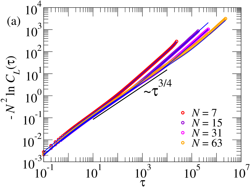
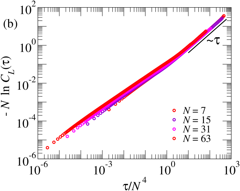
Figure 1: (a) At intermediate times the end-to-end autocorrelation function $C_{L}(\tau)$ exhibits stretched exponential behavior with exponent $\tau^{3/4}/N^{2}$. Note that the persistence length of dsDNA corresponds to $N=114$ in dimensionless units. The simulation data are represented by points, while the solid blue lines, in excellent agreement with the simulation data, represent the corresponding the combined effect of the mode-sums (30). Note also that we cannot reliably use the Hessian approximation of the Hamiltonian too much beyond $N=63$. (b) The stretched exponential behavior lasts till the terminal time $\tau^{*}\sim N^{4}$, beyond which the decay becomes exponential in $\tau/N^{3}$.

We now discuss the analytical behavior of the correlation function in the intermediate time regime and focus on the transverse modes, being the most interesting. The deviation of the correlation from its initial value reads

$$1-\frac{C_{L}(\tau)}{C_{L}(0)}\simeq\frac{16T^{*}}{b^{2}N^{3}}\sum_{p=3,5,\cdots}\frac{1}{\zeta^{t}_{p}}[1-\exp(-\zeta^{t}_{p}\tau)].$$ (31)

Sums of the type (31) are typical for the correlation functions that we consider. They are worked out in Appendix A. With the function $F_{0}(\tau)$ defined in Eq. (A1) and the result (A6) we get

$$1-\frac{C_{L}(\tau)}{C_{L}(0)}\simeq\frac{16T^{*}}{b^{2}N^{3}}F_{0}(\tau)\simeq\Gamma(1/4)\frac{8T^{*}\tau^{3/4}}{3\pi b^{2}N^{2}\nu^{1/4}}.$$ (32)

So at intermediate times, where the deviations of the initial value are still small, the correlation function decays in time as a stretched exponential:

$$C_{L}(\tau)\simeq C_{L}(0)\,\exp\left[-\Gamma(1/4)\frac{8T^{*}\tau^{3/4}}{3\pi b^{2}N^{2}\nu^{1/4}}\right].$$ (33)

We note that in the exponent of (33), combination $T^{*}\tau^{3/4}/N^{2}$ can be written as the ratio $(N/l_{p})[\tau^{1/4}/N]^{3}$. Since $N/l_{p}$ is of order 1 in the region of our interest, the ratio is a function of $[\tau/\tau^{*}]^{3}$ with $\tau^{*}=N^{4}$, which is of the order of the slowest transverse decay time $1/\zeta^{t}_{2}$. So the stretched exponential behavior crosses over to exponential decay after time $\tau^{*}$. Note that, due to numerical factors, $\tau^{*}$ is still small in comparison to $1/D_{r}$, which scales as $N^{3}/T^{*}$.

As we corroborate the stretched exponential behavior of $C_{L}(\tau)$ by means of direct simulations in Fig. 1, we note that apart from the mode sum (16) the stretched exponential behavior can be obtained by the following simple argument. First, $C_{L}(\tau)=1-\langle[{\mathbf{L}}(\tau)-{\mathbf{L}}(0)]^{2}\rangle/(2\langle L^{2}(0)\rangle)\sim 1-\langle[{\mathbf{L}}(\tau)-{\mathbf{L}}(0)]^{2}\rangle/(2N^{2})$ is an identity. Next, in time $\tau_{0}\sim 1$, independent of its length, the chain ends move in real space by order $N^{0}$; i.e., $\langle[{\mathbf{L}}(\tau_{0})-{\mathbf{L}}(0)]^{2}\rangle\sim N^{0}$, and consequently, $-\log C_{L}(\tau_{0})\sim 1/N^{2}$. Further, beyond time $\tau^{*}\sim N^{4}$ the correlation function decays exponentially due to rotational diffusion dynamics with diffusion coefficient $D_{r}\sim N^{-3}$ leading to $-\log C_{L}(\tau^{*})\sim N$. Thus, if one assumes that the $-\log C_{L}(\tau)$ values at $\tau_{0}\sim 1$ and at $\tau^{*}\sim N^{4}$ are bridged by an exponential function of a single character, then the only solution is a stretched exponential with exponent $\tau^{3/4}/N^{2}$. These arguments are confirmed in Fig. 1.

IV.2 The autocorrelation function for the middle bond vector

We now evaluate the autocorrelation function for the middle bond vector analytically in the linearized approximation.

For the autocorrelation function for the middle bond vector we consider a chain with an even number of beads, i.e., $N$ is odd. Like the case of the end-to-end vector, the middle bond vector ${\mathbf{u}}_{m}(\tau)$ is described as

$${\mathbf{u}}_{m}(\tau)={\mathbf{u}}_{m}^{(0)}(\tau)+\sum_{p}u_{p}{\mathbf{\Psi}}_{p}(\tau)={\mathbf{u}}_{m}^{(0)}(\tau)+\sum_{p}\left[\phi_{p}^{(N+1)/2}-\phi_{p}^{(N-1)/2}\right]{\mathbf{\Psi}}_{p}(\tau).$$ (34)

Here ${\mathbf{u}}_{m}^{(0)}(\tau)$ is the middle bond vector for the reference groundstate configuration (straight rod). Once again, ${\mathbf{u}}_{m}$ is odd under reversal of the numbering of the beads, so the even modes do not contribute to the sum (34). Comparing Eqs. (8) and (10) we get

$$u_{p}=\phi^{(N+1)/2}_{p}-\phi^{(N-1)/2}_{p}\simeq-2\left(\frac{2}{N+1}\right)^{1/2}\sin\left(\frac{p\pi}{2}\right)\sin\left[\frac{p\pi}{2(N+1)}\right],$$ (35)

where the second identity in Eq. (35) is strict for the longitudinal components and approximate for the transverse ones.

Beyond the time $\tau^{*}$, since the vector ${\mathbf{u}}_{m}^{(0)}(\tau)$ in the reference groundstate undergoes the same rotational diffusion, the expression for the autocorrelation function for the middle bond vector $C_{m}(\tau)=\langle{\mathbf{u}}_{m}(\tau)\cdot{\mathbf{u}}_{m}(0)\rangle/\langle u^{2}_{m}(0)\rangle$ is similar to those for the end-to-end vector, allowing us to write

$$C_{m}(\tau)=\frac{1+\sum_{p\in\text{odd}}\,[u^{2}_{p}\,T^{*}]/[(u^{(0)}_{m})^{2}\zeta_{p}]\,\exp(-\zeta_{p}\tau)}{1+\sum_{p\in\text{odd}}\,[u^{2}_{p}\,T^{*}]/[(u^{(0)}_{m})^{2}\zeta_{p}]}\exp(-2D_{r}\tau),$$ (36)

wherein, once again, the sum does not include $p=1$ transverse modes, and each value of $p$ for the transverse modes needs to be counted twice.

The analysis of the sum over the slow modes is given in the Appendix. With the function $F_{2}(\tau)$ defined in Eq. (A1) and the result (A7) we get

$$C_{m}(0)-C_{m}(\tau)\simeq\frac{\pi^{2}T^{*}}{3I}F_{2}(\tau)\simeq\Gamma(3/4)\frac{N^{3}T^{*}\tau^{1/4}}{6\pi I\nu^{3/4}}.$$ (37)

This gives a stretched exponential

$$C_{m}(\tau)\simeq\exp\left[-\Gamma(3/4)\frac{T^{*}N^{3}\tau^{1/4}}{6\pi I\nu^{3/4}}\right],$$ (38)

In order to appreciate the time regime in which this stretched exponent features we note again that the factor $T^{*}$ effectively counts as a factor $N^{-1}$ and that the exponential behavior lasts up to $\tau^{*}\sim N^{4}$. In that time span the exponent is of order unity and after $\tau^{*}$ the correlation follows the diffusive behavior of the end-to-end vector.

The verification of this result can be found in Fig. 2, which also demonstrates that the mode sum (38) exhibits strong finite-size effects, i.e. the sum and the asymptotic fractional power differ substantially. This is purely an issue related to the sum (36) — the sum can be carried out for indefinitely large values of $N$ (but $N$ cannot be indefinitely increased in simulations, as, given that $l_{p}=114$ in dimensionless units, we cannot reliably use the Hessian approximation of the Hamiltonian too much beyond $N=63$) — and as can be seen in Fig. 2, with increasing $N$ the mode sum (36) does indeed approach the expected stretched exponential behavior (38).

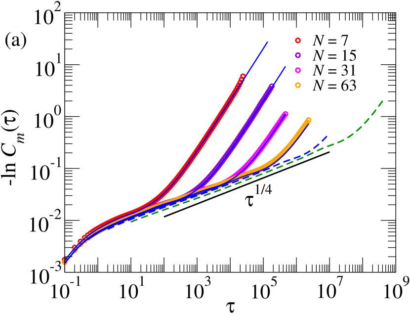
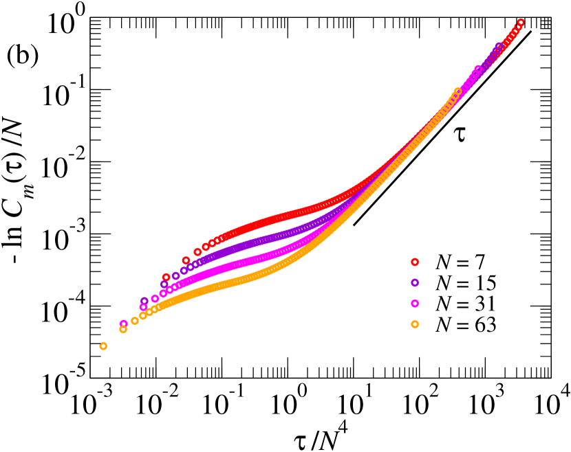
Figure 2: (a) At intermediate times the end-to-end autocorrelation function $C_{m}(\tau)$ exhibits stretched exponential behavior with exponent $\tau^{1/4}$. The simulation data are represented by points, while the solid blue lines, in excellent agreement with the simulation data, represent the corresponding mode sums (36). The blue and green dashed lines correspond to the mode sum (36) for $N=127$ and $N=255$ respectively. (b) The stretched exponential behavior lasts till the terminal time $\tau^{*}\sim N^{4}$, beyond which the decay becomes exponential in $\tau/N^{3}$.

Like in the case of $C_{L}(\tau)$, the stretched exponential behavior for $C_{m}(\tau)$ between $\tau\sim O(1)$ and $\tau=\tau^{*}$ can also be argued from the real-space mean-square displacement of the middle bead in the following manner. First, $C_{m}(\tau)=1-2\langle[{\mathbf{u}}_{m}(\tau)-{\mathbf{u}}_{m}(0)]^{2}\rangle/\langle u_{m}^{2}(0)\rangle\sim 1-2\langle[{\mathbf{u}}_{m}(\tau)-{\mathbf{u}}_{m}(0)]^{2}\rangle/N^{0}$ is an identity. Next, in time $\tau_{0}\sim 1$ the two beads connecting the middle bond vector move in real space by order $N^{0}$; i.e., $\langle[{\mathbf{u}}_{m}(\tau_{0})-{\mathbf{u}}_{m}(0)]^{2}\rangle\sim N^{0}$, and consequently, $-\log C_{m}(\tau_{0})\sim N^{0}$. Further, beyond time $\tau^{*}\sim N^{4}$ the middle bond vector must undergo rotational diffusion with diffusion coefficient $D_{r}\sim N^{-3}$, leading to the result $-\log C_{m}(\tau^{*})\sim N$. Thus, if one assumes that $-\log C_{m}(\tau)$ values at $\tau_{0}\sim 1$ and at $\tau^{*}\sim N^{4}$ are bridged by an exponential function of a single character, then the only solution is a stretched exponential with exponent $1/4$. These arguments are confirmed in Fig. 2.

IV.3 The mean-square displacement of the middle bead

Finally, we evaluate the mean-square displacement of the middle bead in the linearized approximation.

In order to avoid setting up additional simulations for chains with odd number of beads, we continue in this section with chain with even number of beads. We are then interested in the MSD of the center-of-mass of the two middlemost beads; i.e., the mean ${\mathbf{r}}_{m}(\tau)$ of the location of the $(N-1)/2$ and $(N+1)/2$-th beads, ${\mathbf{r}}_{m}(\tau)=\frac{1}{2}[{\mathbf{r}}_{(N+1)/2}(\tau)+{\mathbf{r}}_{(N-1)/2}(\tau)]$ and express it in terms of the modes as

$${\mathbf{r}}_{m}(\tau)\!={\mathbf{R}}_{\text{cm}}(\tau)+\sum_{p}r_{p}{\mathbf{\Psi}}_{p}(\tau)\equiv{\mathbf{R}}_{\text{cm}}(\tau)+\!\tilde{\mathbf{r}}_{m}(\tau),$$ (39)

since, as noted before, the instantaneous location of the midpoint of the reference groundstate coincides with that of the chain’s center-of-mass. The corresponding mode coefficient is then given by

$$r_{p}=\phi^{(N+1)/2}_{p}+\phi^{(N-1)/2}_{p}\simeq 2\left(\frac{2}{N+1}\right)^{1/2}\cos\left(\frac{p\pi}{2}\right)\cos\left[\frac{p\pi}{2(N+1)}\right],$$ (40)

where the second identity in Eq. (39) is strict for the longitudinal components and approximate for the transverse ones.

The MSD of the middle bead is the sum of two terms

$$\langle\Delta r_{m}^{2}(\tau)\rangle=\langle[\Delta\mathbf{R}_{\text{cm}}(\tau)]^{2}\rangle+\langle[\Delta\tilde{\mathbf{r}}_{m}(\tau)]^{2}\rangle,$$ (41)

as the cross terms vanish because the center-of-mass motion of the chain is independent of the internal motion represented by $\tilde{\mathbf{r}}_{m}(\tau)$. The center-of-mass diffuses with coefficient $D\sim 1/N$

$$\langle[\Delta\mathbf{R}_{\text{cm}}(\tau)]^{2}\rangle=4D\tau$$ (42)

and the internal MSD

$$\langle\Delta\tilde{r}_{m}^{2}(\tau)\rangle=\langle[\tilde{\mathbf{r}}_{m}(\tau)-\tilde{\mathbf{r}}_{m}(0)]^{2}\rangle,$$ (43)

can be computed from the mode sums as above. From the definition it is clear that $\langle\Delta\tilde{r}_{m}^{2}(\tau)\rangle$ must asymptotically approach a constant.

Since the modes are independent of each other at all times, using Eqs. (40-41) we have

$$\langle\Delta\tilde{r}_{m}^{2}(\tau)\rangle=2\sum_{p}\frac{T^{*}}{4\zeta_{p}}\left[\phi_{p}^{(N+1)/2}+\phi_{p}^{(N-1)/2}\right]^{2}\left[1-\exp(-\zeta_{p}\tau)\right],$$ (44)

which is evaluated in the Appendix. Only the even modes contribute to the sum, and it is once again dominated by the transverse modes, with the result that at intermediate times

$$\langle\Delta\tilde{r}_{m}^{2}(\tau)\rangle=\Gamma(1/4)\frac{4T^{*}\tau^{3/4}}{3\pi\nu^{1/4}},$$ (45)

i.e., it increases subdiffusively in time with an exponent $3/4$. The subdiffusive behavior is seen until time $\tau^{*}$, beyond which it saturates. The verification of this result can be found in Fig. 3, which, like Fig. 2, also demonstrates that the conversion of the mode sum (30) to integrals suffers from strong finite-size effects; with increasing $N$ the mode sum (30) does approach the expected subdiffusive behavior (44).

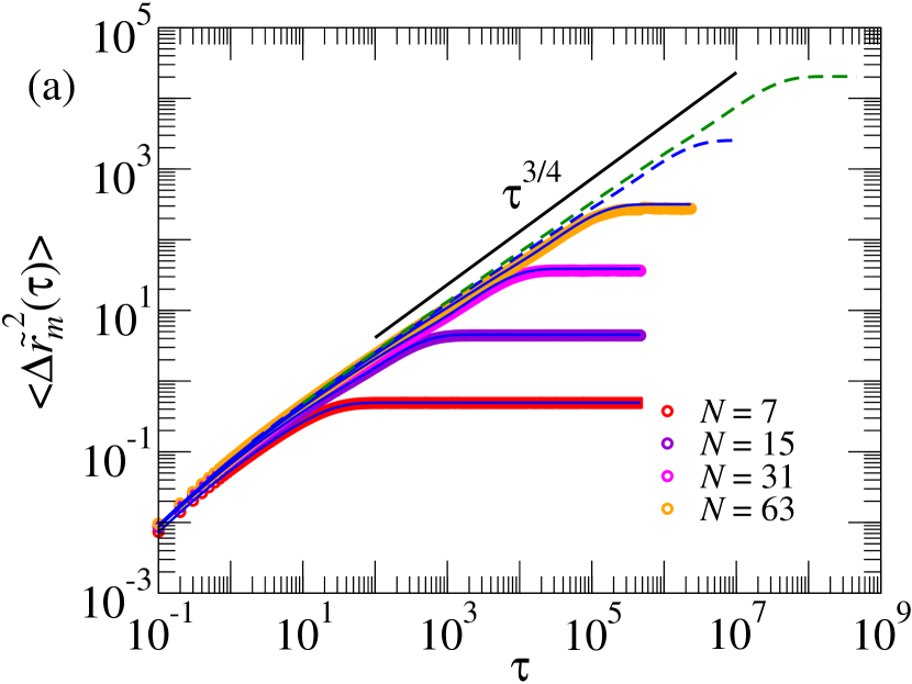
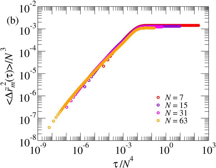
Figure 3: (a) At intermediate times $\langle\Delta\tilde{r}_{m}^{2}(\tau)$ increases subdiffusively with exponent $3/4$. The simulation data are represented by points, while the solid blue lines, in excellent agreement with the simulation data, represent the corresponding mode sums (44). The blue and green dashed lines correspond to the mode sum (44) for $N=127$ and $N=255$ respectively. (b) The subdiffusive behavior lasts till the terminal time $\tau^{*}\sim N^{4}$, beyond which the data flatten out as they should.

The subdiffusive behavior with exponent $3/4$ can also be argued in the following manner. In time $\tau_{0}\sim 1$ the center-of-mass of the two middlemost beads moves by a distance of $N^{0}$ due to the internal motion, i.e. the MSD is of order $N^{0}$. Around $\tau^{*}\sim N^{4}$ the center-of-mass motion starts to dominate and the MSD becomes order $D\tau^{*}\sim\tau^{*}/N\sim N^{3}$. If the two values are to be bridged by a single power-law, then the only possible exponent is $3/4$.

IV.4 Mode sums vs stretched exponents

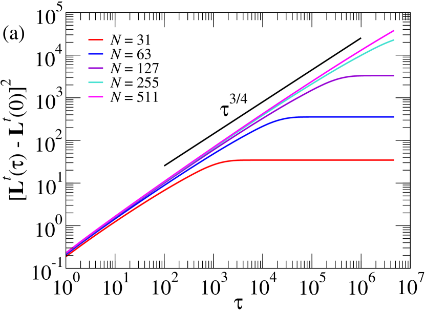
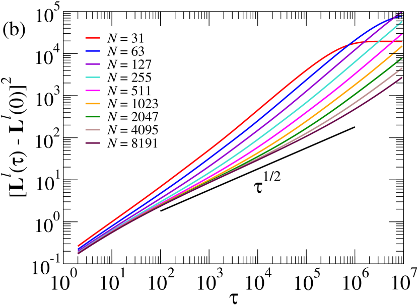
Figure 4: (a) Log-log plot of the transverse MSD of the end-to-end vector as given by the expression (30) for a series of lengths. For comparison the anticipated power $\tau^{3/4}$ has been drawn. (b) Log-log plot of the longitudinal MSD of the end-to-end vector as given by the expression (30) for a series of lengths. The convergence to the anticipated power $\tau^{1/2}$ is too slow to be useful.

In the previous subsections, we have extracted stretched exponents from the mode sums by replacing the sums over the mode index $p$ by integrals and approximating the modes by their low-$p$ behavior as given in (6) and (7). Since our interest is in chain lengths shorter than or comparable to the persistence length, it is important to know how well the mode sums converge to this asymptotic behavior. In Fig. 4 we have plotted the transverse mode sums for the MSD of the end-to-end vector, for a set of chain lengths shorter and longer than the persistence length $l_{p}=114$ (for the dsDNA parameters $T^{*}=0.034$ and $\nu=0.35$). The figure shows that the mode sums, in the intermediate time regime $\tau\ll\tau^{*}$, are very well represented by the power $\tau^{3/4}$ over a large time domain, also for chains of the order of the persistence length. The time domain, for which the stretched exponent holds, expands with $N$.

In the same Fig. 4 the longitudinal mode sums for the MSD of the end-to-end vector are plotted. Here one observes that the convergence to the anticipated power $\tau^{1/2}$ is very slow. ($\tau^{1/2}$ follows from the replacement of the sum by an integral). Even a chain of length of $N=8191$, which is about 75 times the persistence length, cannot be represented in a substantial time domain by the power $\tau^{1/2}$. This is one of the reason that we have concentrated in the previous sections on the analysis of the transverse mode sums. The other reason is that the contribution of the longitudinal modes in the total end-to-end vector remains small, since the transverse modes dominate for intermediate times and the orientational diffusion takes over for long times.

IV.5 Summary statements on linearized dynamics

We now close off linearized semiflexible polymer dynamics with a summary.

Based on the linearized dynamics for our model we have obtained analytical expressions for (i) the autocorrelation function of the end-to-end vector, (ii) the autocorrelation function of a bond (i.e., a spring, or a tangent) vector at the middle of the chain and (iii) the mean-square displacement of a tagged bead in the middle of the chain, as sum over the contributions from the transverse and/or longitudinal modes — the so-called mode sums. The mode sum exhibit the following asymptotic behavior. (i) The end-to-end vector autocorrelation function for the chain decays in time as a stretched exponential with an exponent $3/4$, crossing over to pure exponential decay at the terminal time $\tau^{*}=(\zeta_{2}^{t})^{-1}$. (ii) The autocorrelation of the orientation of the middlemost bond vector decays in time in a similar manner, but with an exponent $1/4$. (iii) The mean-square displacement (MSD) of the middle bead shows anomalous diffusion with an exponent $3/4$ until time $\tau^{*}$, beyond which its motion becomes diffusive. The convergence with increasing $N$ to the asymptotic power is fast for the transverse mode sum and very slow for the longitudinal mode sum.

Further, dynamical quantities as obtained from mode sums show a remarkable agreement with numerical simulation results of dsDNA chains with lengths shorter or of the order of the persistence length. The main exceptions to this agreement stem from the fact that if the chain bends, it tends to conserve its curvilinear length, thereby reducing the distance between the ends. The mode sums do not capture this effect, which is nonlinear and a consequence of coupling between the transverse and longitudinal modes. This is discussed in more detail in Sec. V.

V Separating the longitudinal and transverse components

In the previous section we have compared the results of linearized dynamics with the simulations, involving the full polymer dynamics of the model in terms of three correlation functions. The observed excellent agreement suggests that for lengths less than $l_{p}$ the linearized dynamics suffices, which opens up a wide avenue of opportunity for analytical calculations using our model. In this and the next sections we will examine this agreement in further detail, taking the end-to-end vector as an example.

The end-to-end vector correlation function calculations in Fig. 1 (and other quantities) did not need a distinction between longitudinal and transverse fluctuations, hence the simulations for these quantities can be carried out with any integration scheme, including the integration of equations (12) employing the positions of the beads. As we now embark on separating the longitudinal and transverse fluctuations, the polymer dynamics in the simulations requires more care, in particular the role of the coupling forces and the orientation of the groundstate, as will be described below.

The coupling force arises from the derivative of the contour length $L_{c}$ and in terms of the mode representation, we have

$${\bf H}_{p}=\sum_{n}\left[\frac{\partial L_{c}}{\partial{\bf r}_{n}}-\left(\frac{\partial L_{c}}{\partial{\bf r}_{n}}\right)^{(0)}\right]\,\phi_{n,p}.$$ (46)

Having worked out the partial derivatives we find for the longitudinal component

$${\mathbf{H}}^{l}_{p}=\sum_{n}\left(\hat{\bf u}_{n}-\hat{\bf u}^{(0)}_{n}\right)^{l}\left[\phi^{l}_{n,p}-\phi^{l}_{n-1,p}\right]$$ (47)

and for the transverse components

$${\bf H}^{t}_{p}=\sum_{n}{\bf u}^{t}_{n}\left(\frac{1}{u_{n}}-\frac{1}{u^{(0)}_{n}}\right)\left[\phi^{t}_{n,p}-\phi^{t}_{n-1,p}\right].$$ (48)

It is worthwhile to note that the longitudinal coupling force arises from the transverse fluctuations — a pure longitudinal deformation will not change the direction $\hat{\bf u}_{n}$, as occurring in Eq. (47), from that in the groundstate $\hat{\bf u}^{(0)}_{n}$. This is also reflected in the fact that the longitudinal modes are exact eigenmodes of the system in the groundstate.

The simulation is carried out by forward-integrating Eq. (13). For the integration we represent the chain configurations by continuously alternating between the mode representation (for the timestep) and the position representation (for the calculation of the coupling forces). For the longitudinal components the transformation back and forth between the mode representation and position representation is a (fast) Fourier Transform. For the transverse components the back and forth transformations are found using the transverse eigenfunctions $\phi^{t}_{n,p}$.

As discussed in Sec. II.3, the groundstate is identified by enforcing the components of the transverse modes for $p=1$ strictly equal to zero. This condition must be satisfied, in principle, at every time step, requiring an adjustment of the orientation of the groundstate, by rotating the direction $\hat{\bf e}_{0}$ around an axis $\bf\omega$ perpendicular $\hat{\bf e}_{0}$. The adjustment of the orientation of the groundstate leaves the spatial configuration of the beads invariant, but induces a transformation of its representation in modes. The direction of $\bf\omega$ as well as details of the transformation are provided in Appendix B.

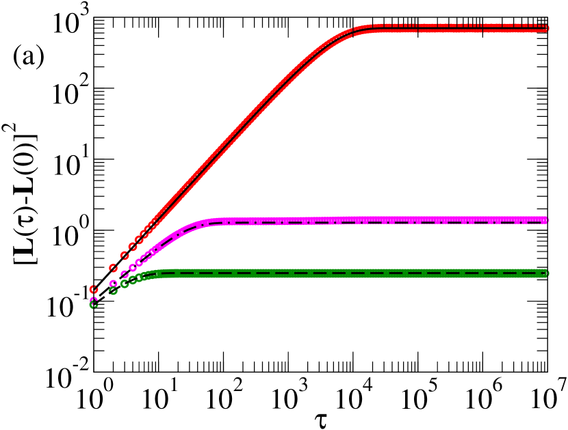
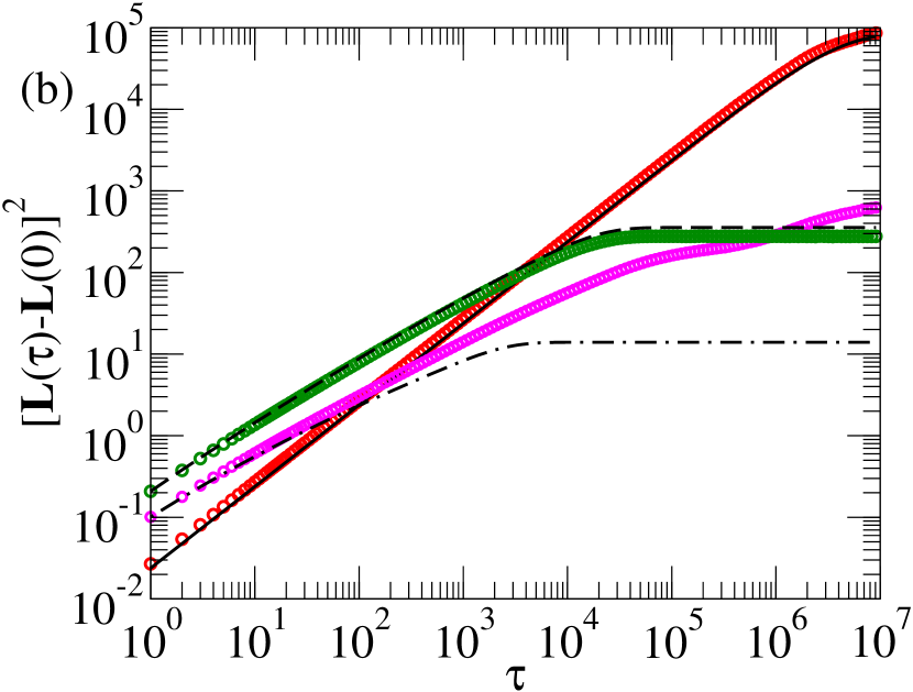
Figure 5: The orientational, longitudinal and transverse components of the mean-square displacements $[{\bf L}^{(0)}(\tau)-{\bf L}^{(0)}(0)]^{2}$ (linearized theoretical results in solid lines and simulation data in red symbols), $[{\bf L}^{l}(\tau)-{\bf L}^{l}(0)]^{2}$ (linearized theoretical results in dash-dotted lines and simulation data in magenta symbols), and $[{\bf L}^{t}(\tau)-{\bf L}^{t}(0)]^{2}$ (linearized theoretical results in dashed lines and simulation data in green symbols) respectively: (a) $N=7$, (b) $N=63$.

The linearized theoretical results and the simulation data for the orientational, longitudinal and transverse components of the mean-square displacements $[{\bf L}^{(0)}(\tau)-{\bf L}^{(0)}(0)]^{2}$, $[{\bf L}^{l}(\tau)-{\bf L}^{l}(0)]^{2}$ and $[{\bf L}^{t}(\tau)-{\bf L}^{t}(0)]^{2}$ respectively [see Eq. (21) for the definitions] are compared for $N=7$ and $63$ for dsDNA in Fig. 5. For very short chains (such as $N=7$) the coupling force stays small in amplitude, explaining the excellent agreement between the simulations and the linearized dynamics results. For $N=63$ however, we see that at long times, the agreement between the linearized theory and the simulation is rather poor for the longitudinal component $[{\bf L}^{l}(\tau)-{\bf L}^{l}(0)]^{2}$. Despite this disagreement, we clearly see in Fig. 5(b) that in the region of the strongest disagreement the orientational component $[{\bf L}^{(0)}(\tau)-{\bf L}^{(0)}(0)]^{2}$ — for which the linearized theoretical results and the simulation data do agree very well — is two orders of magnitude stronger than the longitudinal component $[{\bf L}^{l}(\tau)-{\bf L}^{l}(0)]^{2}$. This observation is therefore consistent with the good agreement between the linearized theoretical results and the simulation data for $C_{L}(\tau)$, wherein all the orientational, longitudinal and transverse components combine together.

Figure 5(b) shows that the main deviations from the linear theory are in the longitudinal component of the end-to-end vector for asymptotic large times. This is a result of the coupling between the longitudinal and the transverse modes. The bending of the chain due to transverse fluctuations shortens the end-to-end distance in the longitudinal direction. The next section is devoted to a further analysis of these effects.

VI Non-linear effects in semiflexible polymer dynamics

Semiflexible polymer dynamics is inherently nonlinear. If the nonlinear effects get strong then they clearly ruin the agreement between the (linearized) mode sums and the simulation data. An interesting question is, why do they show up strongly in longitudinal fluctuations, e.g., in the quantity $[{\bf L}^{l}(\tau)-{\bf L}^{l}(0)]^{2}$?

There are two different classes of situations where we expect the nonlinearities to become strong. (i) The first case is when the chain gets long in comparison to its persistence length. In this case the transverse fluctuations become progressively easier to excite with increasing chain lengths, and the effective chain length along the vector $\hat{\mathbf{e}}_{0}$ that denotes the orientation of the groundstate shortens from ${\bf L}^{(0)}_{0}$. (ii) The second case is when the chain gets progressively more inextensible. In the limit when the chain is completely inextensible, like the WLC model, any transverse fluctuation results in an immediate shortening of the end-to-end distance. This case is best analyzed by reducing $T^{*}$, i.e., reducing the stretchability of the bonds, while simultaneously keeping the persistence length $l_{p}=\nu/T^{*}$ fixed. In this case one expects strong nonlinearities to emerge also in chains that are short with respect to the persistence length. Both cases affect longitudinal fluctuations the most, hence the quantity $[{\bf L}^{l}(\tau)-{\bf L}^{l}(0)]^{2}$ is the most sensitive to nonlinearities in the model.

We first discuss case (i) as a follow-up of $[{\bf L}^{l}(\tau)-{\bf L}^{l}(0)]^{2}$ in Fig. 5 for dsDNA. In order to clearly see the non-linear effects we have plotted in Fig. 6 the simulated values as well as the difference between the simulated values and that given by the corresponding linearized dynamics theory. We see that for short chains the difference remains small, while it grows to substantial values for long chains. This is because the linearized theory predicts that $[{\bf L}^{l}(\tau)-{\bf L}^{l}(0)]^{2}$-values reach a plateau beyond the lifetime of the longitudinal modes as seen in Fig. 5, but the simulated values keep increasing due to nonlinearities [encoded in the coupling force term as described in Eq. (46)]. As already explained above, the main source of this non-linear effect is the shortening of the end-to-end distance along the vector $\hat{\mathbf{e}}_{0}$ due to the transverse fluctuations. Indeed, in support of the arguments given in the above paragraph, we find that with increasing chain lengths the longitudinal modes, in particular those with a low odd index $p$, do not fluctuate around zero any more (as assumed in the linearized dynamics), but around a positive average. If we translate these positive averages back to spatial positions, we find a shorter distance $\langle({\bf r}_{N}-{\bf r}_{0})\cdot\hat{\bf e}_{0}\rangle$ than the groundstate value $L^{(0)}$. The shortening of the distance becomes for longer chains much larger than the amplitude of the longitudinal fluctuations.

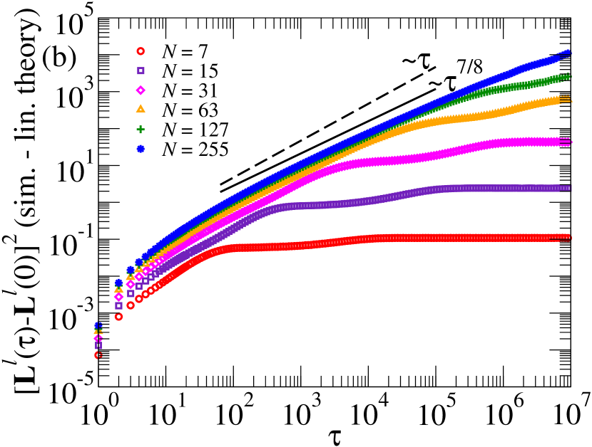
Figure 6: Plots for the longitudinal component of $[{\bf L}^{l}(\tau)-{\bf L}^{l}(0)]^{2}$ for dsDNA for $N=7,15,31,63,127$. and $255$. (a) The total value of $[{\bf L}^{l}(\tau)-{\bf L}^{l}(0)]^{2}$ is plotted; symbols denote simulation data, and solid lines denote the corresponding linearized mode sums for the same values of $N$ as in the simulations (the value of $N$ corresponding to the mode sums increase from bottom to top). The dashed line shows corresponds to the power-law $\tau^{7/8}$. (b) The pure non-linear effect as the difference between the simulated values and the linear contribution given by the mode sum. In the difference the emergence of an effective power-law $\tau^{7/8}$ (solid line) can be seen at intermediate times before leveling off. For comparison, also plotted is a dashed line showing power-law $\tau^{1}$.

An interesting feature of the curves of Fig. 6 is that $[{\bf L}^{l}(\tau)-{\bf L}^{l}(0)]^{2}$ at intermediate times is a combination of the (linear) mode sums and inherently nonlinear behavior of the model. Indeed, the pure nonlinear contributions to $[{\bf L}^{l}(\tau)-{\bf L}^{l}(0)]^{2}$ to an effective power-law $\tau^{7/8}$ at intermediate times before the data level off, as indicated by the straight line in the log-log plot in Fig. 6(b). The mode sum contributions, on the other hand, although very slowly converges to $\tau^{1/2}$ behavior as seen in Fig. 4, we expect an effective exponent less than $7/8$ for $[{\bf L}^{l}(\tau)-{\bf L}^{l}(0)]^{2}$, as confirmed in Fig. 6(a). (We mention in passing here that the nonlinear effects in the longitudinal fluctuations are well-documented in the WLC literature. E.g., for (inextensible) WLC model, a power law in time with exponent $7/8$ is reported for the fluctuations in the longitudinal component of the end-to-end vector hall2 ; liverpool4 ; ober2 — this prompts the comparison of our data in Fig. 6 to a power-law $\tau^{7/8}$. We will return to this in the next section.)

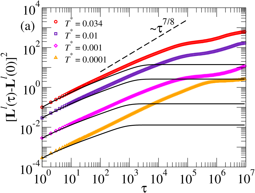
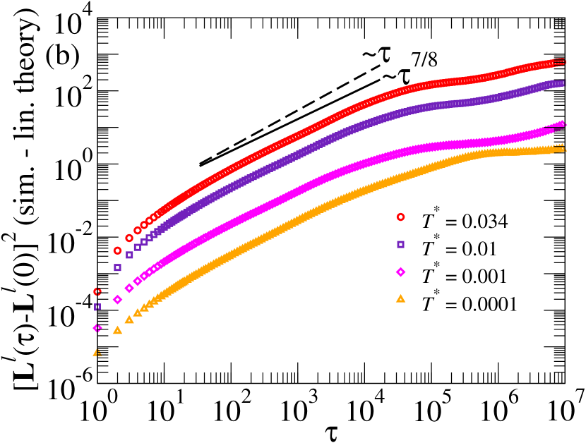
Figure 7: The longitudinal component of the end-to-end vector $[{\bf L}^{l}(\tau)-{\bf L}^{l}(0)]^{2}$ for dsDNA ($T^{*}=0.034$) and a few other values of $T^{*}$. Here $N=63$ and the persistence length is $\approx 114$ nm for all cases. As in Fig. 6 we plot in part (a) the total value of $[{\bf L}^{l}(\tau)-{\bf L}^{l}(0)]^{2}$; symbols denote simulation data, and solid lines denote the corresponding linearized mode sums for the same values of $T^{*}$ as in the simulations (the value of $T^{*}$ corresponding to the mode sums increase from bottom to top), and the dashed line shows corresponds to the power-law $\tau^{7/8}$. in part (b) the difference between the simulation and the linear contribution as given by the mode sum. Again in the difference the emergence of an effective power-law $\tau^{7/8}$ (solid line) can be seen at intermediate times before leveling off. For comparison, also plotted is a dashed line showing power-law $\tau^{1}$.

Case (ii) yields a similar picture. In the limit of small $T^{*}$ (and $l_{p}=\nu/T^{*}$ still fixed at its dsDNA value $\approx 114$ nm), the contribution of the longitudinal fluctuations within the linearized theory vanishes with the power $T^{*}$, since the decay of the modes becomes independent of $\nu$ for $\nu\rightarrow 0$. However the transverse modes, for which the decay coefficients are proportional to $\nu$ [c.f. Eq. (7)], survive longer being proportional to $T^{*}/\nu$. Since the transverse modes for more unstretchable chains imply a shortening of the end-to-end distance with respect to the groundstate, the longitudinal modes again get a non-vanishing average in equilibrium. This is shown in Fig. 7, where we have plotted the longitudinal component of the end-to-end vector for chain length $N=63$ with $l_{p}\approx 114$ nm not only for dsDNA ($T^{*}=0.034$), but also for $T^{*}=0.01,0.001$ and $0.0001$. Again we plot $[{\bf L}^{l}(\tau)-{\bf L}^{l}(0)]^{2}$ as well as the difference between the simulation and the linear contribution as given by the mode sum, and the total. The $[{\bf L}^{l}(\tau)-{\bf L}^{l}(0)]^{2}$ data show an effective exponent less than $7/8$, while the pure nonlinear contributions to $[{\bf L}^{l}(\tau)-{\bf L}^{l}(0)]^{2}$, although initially very small with respect to the total contribution, they grow with time, as an effective power-law $\tau^{7/8}$ at intermediate times, before saturating to different plateau-values for different values of $T^{*}$. We note that it difficult to extract from the total contribution an effective power law, since the linear contribution suffers from large finite size effects as Fig. 4 shows.

Our results for $[{\bf L}^{l}(\tau)-{\bf L}^{l}(0)]^{2}$ bear strong resemblance to those of Refs. recent6 ; ober2 where the extensible WLC has also been shown to demonstrate the exponents $1/2$ and $7/8$ at intermediate times in the dynamic elastic modulus, obtained from the (length fluctuation) response of the chain to a (fluctuating) tensile force. Linear response theory suggests that the dynamic elastic modulus via a memory kernel, must relate to the equilibrium fluctuations in the longitudinal end-to-end vector studied by ourselves. For tagged monomer displacement, such a case has been studied in detail by one of us panja1 ; panja2 by means of Generalized Langevin Equation (GLE) formulation. In the present case however, we do not know how to quantitatively relate our results for the mean-square displace longitudinal end-to-end vector and those of Refs. recent6 ; ober2 using a GLE, or some other, formulation.

We again emphasize here that even at the times when the nonlinear contribution to $[{\bf L}^{l}(\tau)-{\bf L}^{l}(0)]^{2}$ become significant, it still remains typically two orders of magnitude smaller than the orientational component $[{\bf L}^{(0)}(\tau)-{\bf L}^{(0)}(0)]^{2}$, so nonlinearities make little difference for the quantities dependent on the overall end-to-end vector. It is in this sense we state, in view of Figs. 1-5 that the linearized dynamics suffices very well for dsDNA fragments that are shorter than or comparable to the persistence length.

VII Conclusion

With a recently introduced Hamiltonian bead-spring model for semiflexible polymers hans , in this paper we have studied the dynamical properties of a chain of length $N$. Specifically, using linearized polymer dynamics we have analytically calculated the autocorrelation functions of the end-to-end vector, that of the orientation of the middle bond and the mean-square displacement of the middlemost bead of the chain. The analytical solutions are facilitated by the fact that we know the dynamical mode structures analytically in the Hessian approximation of the Hamiltonian. There are longitudinal and transverse modes, and the terminal time $\tau^{*}\sim N^{4}$ is determined as the inverse of the smallest eigenvalue $\zeta^{t}_{2}$ for the transverse modes. Up to time $\tau^{*}$ the autocorrelation functions for the end-to-end vector and that of the middle spring vector show stretched exponential behavior with exponents $3/4$ and $1/4$ respectively, and beyond time $\tau^{*}$ the decay becomes simply exponential. The motion of the middlemost bead exhibit anomalous dynamics with an exponent $3/4$ until time $\tau^{*}$, and is diffusive thereafter.

The full dynamics of semiflexible polymers in our model is obviously nonlinear, and we have also performed simulations of the full dynamics for chains. We find that for dsDNA the mode sums agree remarkably well with the numerical values obtained from simulations. This does not however mean that the nonlinearities are not present. Indeed, we find that the MSD of the longitudinal component of the end-to-end vector showcases strong nonlinear effects in the polymer dynamics, and we identify at least an effective $t^{7/8}$ power-law regime in its time-dependence. We show that the nonlinear effects in the MSD of the longitudinal component of the end-to-end vector increases with increasing length for dsDNA; nevertheless, in comparison to the full mean-square displacement of the end-to-end vector the nonlinear effects remain small at all times. It is in this sense we state that the linearized dynamics suffices for dsDNA fragments that are shorter than or comparable to the persistence length.

Given that the worm-like chain (WLC) is the most used model for semiflexible polymers, it is imperative to compare the results of the above quantities across the two models. First of all, the anomalous dynamics of the middlemost bead agree for the two models kroy ; farge , and have also been found in experiments expt1 ; expt2 ; expt3 . On the other hand, the end-to-end vector correlation function has been considered in Ref. liverpool4 , wherein $\langle[{\mathbf{L}}(t)-{\mathbf{L}}(0)]^{2}\rangle$ is seen to behave as $A_{1}t^{3/4}+A_{2}t^{7/8}$, with $A_{1}$ and $A_{2}$ two $N$-dependent constants, of which the $t^{7/8}$ term is known to originate from nonlinear effects in WLC dynamics, and showcases itself in the longitudinal fluctuations of the end-to-end vector. The form of the term proportional to $A_{1}$ is consistent with the stretched exponential behavior (33) when $\tau\ll\tau^{*}$ [since $\exp(-Bx^{\alpha})\approx 1-Bx^{\alpha}$ for $Bx^{\alpha}\ll 1$]. Further, we have also found at least an apparent $t^{7/8}$ power-law in the longitudinal MSD of the end-to-end vector, albeit with an almost insignificant amplitude wrt the overall fluctuations of the end-to-end vector (we cannot ascertain a true power-law behavior since we do not have an analytical derivation for $t^{7/8}$). Further, Ref. liverpool4 reports the orientational correlation function of the unit tangent vector at the middle of the chain, which is analogous to that of the orientation of the middle bond vector ${\mathbf{u}}_{m}$ in our model. The corresponding result, translated in terms of ${\mathbf{u}}_{m}$ would imply that $\langle[{\mathbf{u}}_{m}(t)-{\mathbf{u}}_{m}(0)]^{2}\rangle=B_{1}t^{1/4}+B_{2}t^{1/2}$, with $B_{1}$ and $B_{2}$ two $N$-dependent constants. The form of the term proportional to $B_{1}$ is consistent with the stretched exponential behavior (33) at $t\ll\tau^{*}$, but we do not find any signature of an exponent $1/2$ for $\langle[{\mathbf{u}}_{m}(t)-{\mathbf{u}}_{m}(0)]^{2}\rangle$ in our result. It is of course possible that the $t^{1/2}$ behavior arises from the (nonlinear) longitudinal fluctuations, which, in light of the longitudinal fluctuations in the end-to-end vectors, we also expect to have an almost insignificant impact on the total fluctuations in ${\mathbf{u}}_{m}(t)$. We have already shown results for $N=255$ for dsDNA in one occasion (6) — an instance where we are able to simulate, at the basepair resolution, full chains of length more than twice the persistence length.

Appendix A The stretched exponentials derived from the mode-sums

In this appendix we present some formulas that enable us to analyze $C_{L}(t)$. We start with sums of the type

$$F_{n}(\tau)=\sum_{p=3,}\frac{p^{n}}{\zeta^{t}_{p}}[1-\exp(-\zeta^{t}_{p}\tau)]),$$ (A1)

The function $F_{0}(\tau)$ is relevant for the auto-correlation function of the end-to-end vector and the mean squared displacement of the middle bead. The function $F_{2}(\tau)$ is needed for the auto-correlation function of the middle bond, and for next to dominant contributions. The first step is to replace the sum by an integral. The justification comes from the fact that for small values of the exponent (which is the case for $\tau\leq\tau^{*}=N^{4}$) a large range of $p$-values contribute, for which the integrand is smoothly varying. So, we approximate $F_{0}(\tau)$ by

$$F_{n}(\tau)\simeq\frac{1}{2}\int dp\frac{p^{n}}{\zeta^{t}_{p}}[1-\exp(-\zeta^{t}_{p}\tau)]),$$ (A2)

Next we approximate $\zeta^{t}_{p}$ in the regime where the main contributions come from by

$$\zeta^{t}_{p}\simeq\frac{\nu\pi^{4}p^{4}}{N^{4}}$$ (A3)

and make the substitution

$$p=\frac{N}{\pi(\nu\tau)^{1/4}}q^{1/4},$$ (A4)

which leads for $F_{0}(\tau)$ to the integral

$$F_{0}(\tau)\simeq\frac{N\tau^{3/4}}{8\pi\nu^{1/4}}\int dq\,q^{-7/4}[1-\exp(-q)].$$ (A5)

Integration by parts gives the result

$$F_{0}(\tau)\simeq\frac{N\tau^{3/4}}{6\pi\nu^{1/4}}\int dq\,q^{-3/4}\exp(-q)=\frac{N\tau^{3/4}}{6\pi\nu^{1/4}}\Gamma(1/4).$$ (A6)

For $F_{2}(\tau)$ the derivation is similar. Only the front factor and the power of $\tau$ differ:

$$F_{2}(\tau)\simeq\frac{N^{3}\tau^{1/4}}{2\pi^{3}\nu^{3/4}}\Gamma(3/4).$$ (A7)

In Section IV.1 the interplay between the front factors and the time dependence has been discussed with the result that times $\tau\sim N^{4}$ are most relevant for the exponent of the stretched exponential. As follows, one can see that the next order $\sim p^{2}$ in the expansion of $L_{p}$ is dwarfed by Eq. (A6). The term has an extra factor $N^{2}$ in the denominator and gets another extra factor $N^{2}$ in the numerator as $F_{0}$ has to be replaced by $F_{2}$ (with the second extra factor). But $\tau^{3/4}$ in $F_{0}$ gives a factor $N^{3}$ for $\tau\sim\tau^{*}$ and $\tau^{1/4}$ in $F_{2}$ gives a factor $N$. So the next term in the expansion is a factor $N^{-2}$ smaller than the dominant term.

The contribution of the longitudinal modes cannot be observed for similar reasons. The analysis with the spectrum $\zeta^{l}_{p}\sim(p/N)^{2}$ gives the combination $\tau^{1/2}N^{-2}$, which applies for times bounded by $(\zeta^{l}_{1})\sim N^{2}$. Hence, the combination $\tau^{1/2}N^{-2}$ remains very small in that time regime.

Appendix B Adjustment of the reference groundstate

In this appendix we discuss the adjustment of the reference groundstate such that the transverse mode $p=1$ are kept equal to zero. The adjustment amounts to a rotation of the vectors ${\bf r}^{0}_{n}$ over an angle $\theta$ around an axis $\hat{\bf\omega}$. With this $\hat{\bf\omega}$ and $\theta$ the set of reference axes $\hat{\bf e}_{\alpha}$ are rotated to a system $\hat{\bf e}^{R}_{\alpha}$ connected to the original ones by the matrix

$$\hat{\bf e}^{R}_{\alpha}=\sum_{\beta}T_{\alpha,\beta}\,\hat{\bf e}_{\beta}.$$ (B1)

The matrix $T_{\alpha,\beta}$ is related to the rotation $\hat{\bf\omega},\theta$ by

$$T_{\alpha,\beta}=\cos\theta\,\delta_{\alpha,\beta}+(1-\cos\theta)\,\omega_{\alpha}\omega_{\beta}+\sin\theta\,\omega_{\alpha\times\beta}.$$ (B2)

Here $\omega_{\alpha}$ is the component $\alpha$ of the vector $\hat{\bf\omega}$. The index $\alpha\times\beta$ means for $\alpha\neq\beta$ the next one in the periodic series $0,1,2,0,1,\dots$ with $\omega_{\beta\times\alpha}=-\omega_{\alpha\times\beta}$. As $\hat{\omega}$ is a unit vector one has the relation

$$\sum_{\alpha}\,\omega^{2}_{\alpha}=1.$$ (B3)

There is no point of rotating the vectors ${\bf r}^{0}_{n}$ around their common direction, so we put $\omega_{0}=0$.

The problem is to find the two other components $\omega_{1}$ and $\omega_{2}$ which have the role to let the modes $\Psi^{1}_{1}$ and $\Psi^{2}_{1}$ vanish. First we derive the transformation of the components of the modes under a general rotation of the reference basis. Note that we rotate the reference basis but keep the positions of the monomers fixed. As the longitudinal and transverse mode behave differently we treat them separately. According to (13) the longitudinal mode is related to the positions in the rotated reference systems as

$$(\Psi^{0}_{p})^{R}=\sum_{n}\left[{\bf r}_{n}\cdot\hat{\bf e}^{R}_{0}-r^{0}_{n}\right]\phi^{l}_{n,p}=\sum_{n}\left[\sum_{\beta}T_{0,\beta}\,({\bf r}_{n}\cdot\hat{\bf e}_{\beta})-r^{0}_{n}\right]\phi^{l}_{n,p}.$$ (B4)

We express, with (11), the components of positions ${\bf r}_{n}$ back into the modes of the original reference system

$${\bf r}_{n}\cdot\hat{\bf e}_{\beta}=r^{0}_{n}\,\delta_{\beta,0}+\sum_{q}\phi^{\beta}_{n,q}\,\Psi^{\beta}_{q}.$$ (B5)

The longitudinal and transverse eigenfunctions are orthogonal for the same type

$$\sum_{n}\phi^{l}_{n,p}\,\phi^{l}_{n,q}=\delta_{p,q}\quad\quad\sum_{n}\phi^{t}_{n,p}\,\phi^{t}_{n,q}=\delta_{p,q},$$ (B6)

but the mixed combination yields the matrix

$$\sum_{n}\phi^{l}_{n,p}\,\phi^{t}_{n,q}=A_{p,q},$$ (B7)

which is nearly diagonal and which has only even-even and odd-odd elements. So we get for the longitudinal modes

$$(\Psi^{0}_{p})^{R}=\sqrt{I}(1-T_{0,0})A_{p,1}+T_{0,0}\,\Psi^{0}_{p}+\sum_{q,\beta=1,2}T_{0,\beta}\,A_{p,q}\,\Psi^{\beta}_{q}.$$ (B8)

We used for the summation over $n$ the explicit form of the eigenfunction of the transverse mode $p=1$ given in (9).

The transverse component transform according to (for $\alpha\neq 0$)

$$(\Psi^{\alpha}_{p})^{R}=\sum_{n}\phi^{t}_{n,p}({\bf r}_{n}\cdot\hat{\bf e}^{R}_{\alpha})=\sum_{n}\phi^{t}_{n,p}\sum_{\beta}T_{\alpha,\beta}({\bf r}_{n}\cdot\hat{\bf e}_{\beta}).$$ (B9)

For the inner product we find

$${\bf r}_{n}\cdot\hat{\bf e}_{\beta}=\delta_{\beta,0}(r^{0}_{n}+\sum_{q}\phi^{l}_{n,q}\Psi^{0}_{q})+(1-\delta_{\beta.0})\sum_{q}\phi^{t}_{n,q}\Psi^{\beta}_{q}.$$ (B10)

Inserting (B10) into (B9) yields, using (9) and (B6),

$$(\Psi^{\alpha}_{p})^{R}=T_{\alpha,0}\,\left(-\sqrt{I}\,\delta_{p,1}+\sum_{q}A_{p,q}\Psi^{0}_{q}\right)+\sum_{\beta=1,2}T_{\alpha,\beta}\Psi^{\beta}_{p}.$$ (B11)

We get an equation for the components $\omega_{1}$ and $\omega_{2}$ by requiring that $(\Psi^{1}_{1})^{R}=(\Psi^{2}_{1})^{R}=0$. In order to make these equations explicit we introduce the combinations

$$u=\frac{\Psi^{1}_{1}}{\sqrt{I}-\sum_{q}A_{p,q}\Psi^{0}_{q}},\quad\quad\quad v=\frac{\Psi^{2}_{1}}{\sqrt{I}-\sum_{q}A_{p,q}\Psi^{0}_{q}}.$$ (B12)

$u$ and $v$ are parameters given by the modes before the rotation of the reference system. The equations for $\omega_{1}$ and $\omega_{2}$ thus obtain the form

$$T_{1,0}=T_{1,1}\,u+T_{1,2}\,v,\quad\quad\quad T_{2,0}=T_{2,1}\,u+T_{2,2}\,v.$$ (B13)

These equations give the components $\omega_{1}$ and $\omega_{2}$ and the angle $\theta$. With the rotation matrix (B2) and $\omega_{0}=0$, we get the explicit equations

$$\left\{\begin{array}[]{rcl}-\sin\theta\,\omega_{2}&=&(1-\cos\theta)\,\omega_{1}\,(\omega_{1}u+\omega_{2}v)+\cos\theta\,u,\\[5.69054pt] \sin\theta\,\omega_{1}&=&(1-\cos\theta)\,\omega_{2}\,(\omega_{1}u+\omega_{2}v)+\cos\theta\,v.\end{array}\right.$$ (B14)

Multiplying the first equation with $\omega_{1}$ and the second with $\omega_{2}$ and adding them gives the equation

$$\omega_{1}\,u+\omega_{2}\,v=0.$$ (B15)

Together with the condition (B3) one finds

$$\omega_{0}=0,\quad\quad\quad\omega_{1}=\frac{v}{\sqrt{u^{2}+v^{2}}},\quad\quad\quad\omega_{2}=-\frac{u}{\sqrt{u^{2}+v^{2}}}.$$ (B16)

Inserting this into (B14) yields the value of $\theta$ or

$$\sin\theta=\frac{\sqrt{u^{2}+v^{2}}}{\sqrt{1+u^{2}+v^{2}}},\quad\quad\quad\cos\theta=\frac{1}{\sqrt{1+u^{2}+v^{2}}}.$$ (B17)

With these values the rotation matrix $T_{\alpha,\beta}$ and the transformation (B8) and (B11) of the modes to the new reference system are determined.

References

- (1) C. Bustamante, J. F. Marko, E. D. Siggia, and S. Smith, Science 265, 1599 (1994).
- (2) J. F. Marko and E. D. Siggia, Macromolecules 28, 8759 (1995).
- (3) M. D. Wang et al., Biophys. J. 72, 1335 (1997).
- (4) A. Ott, M. Magnasco, A. Simon, A. Libchaber, Phys. Rev. E 48, 1642 (1993).
- (5) F. Gittes, B. Mickey, J. Nettleton and J. Howard, J. Cell Biol. 120, 923 (1993).
- (6) O. Kratky and G. Porod, Recl. Trav. Chim. Pays-Bas. 68, 1106 (1949).
- (7) J. J. Hermans and R. Ullman, Physica 18, 951 (1952).
- (8) H. Daniels, Proc. R. Soc. Edinburgh, Sect. A: Math. Phys. Sci. 63, 290 (1952).
- (9) N. Saito, K. Takahashi and Y. Yunoki, J. Phys. Soc. Jpn. 22, 219 (1967).
- (10) H. Yamakawa, Pure Appl. Chem. 46, 135 (1976).
- (11) C. Bouchiat et al., Biophys. J. 76, 409 (1999).
- (12) J. Wilhelm and E. Frey, Phys. Rev. Lett. 77, 2581 (1996).
- (13) J. Samuel and S. Sinha, Phys. Rev. E 66, 050801 (2002).
- (14) A. Dhar and D. Chaudhuri, Phys. Rev. Lett. 89, 065502 (2002).
- (15) P. Gutjahr, R. Lipowsky and J. Kierfeld, Europhys. Lett., 76, 994 (2006).
- (16) B. Obermayer, O. Hallatschek, E. Frey and K. Kroy, Eur. Phys. J. E 23, 375 (2007).
- (17) R.E. Goldstein, S.A. Langer, Phys. Rev. Lett. 75, 1094 (1995).
- (18) N.-K. Lee, D. Thirumalai, Biophys. J. 86, 2641 (2004).
- (19) Y. Bohbot-Raviv, W. Z. Zhao, M. Feingold, C. H. Wiggins, R. Granek, Phys. Rev. Lett. 92, 098101 (2004).
- (20) T. B. Liverpool, Phys. Rev. E 72, 021805 (2005).
- (21) J. T. Bullerjahn, S. Sturm, L. Wolff and K. Kroy, Europhys. Lett. 96, 48005 (2011).
- (22) L. Harnau, R. G. Winkler and P. Reineker, J. Chem. Phys. 104, 6355 (1996).
- (23) R. G. Winkler, J. Chem. Phys. 118, 2919 (2003).
- (24) J. Käs, H. Strey and E. Sackmann, Nature 368, 226 (1994).
- (25) U. Seifert, W. Wintz, and P. Nelson, Phys. Rev. Lett. 77, 5389 (1996).
- (26) A. Ajdari, F. Jülicher, and A. Maggs, J. Phys. (Paris)7, 823 (1997)
- (27) R. Everaers, F. Jülicher, A. Ajdari, and A. C. Maggs, Phys. Rev. Lett. 82, 3717 (1999)
- (28) F. Brochard-Wyart, A. Buguin, and P.-G. de Gennes, Europhys. Lett. 47, 171 (1999)
- (29) O. Hallatschek, E. Frey, and K. Kroy, Phys. Rev. Lett. 94, 077804 (2005).
- (30) G. T. Barkema and J. M. J. van Leeuwen, J. Stat. Mech. P12019 (2012).
- (31) E.M. Huisman, C. Storm and G.T. Barkema, Phys. Rev. E 82, 061902 (2010).
- (32) E. Farge and A. C. Maggs, Macromolecules 26, 5041 (1993).
- (33) C. F. Schmidt, M. Bärmann, G. Isenberg and E. Sackmann, Macromolecules 22, 3638 (1989).
- (34) A. Caspi, M. Elbaum, R. Granek, A. Lachish and D. Zbaida, Phys. Rev. Lett. 80 1106 (1998).
- (35) M. A. Dichtl and E. Sackmann, New J. Phys. 1, 1 (1999).
- (36) B. Obermayer and E. Frey, Phys. Rev. E 80, 040801(R) (2009).
- (37) D. Panja, J. Stat. Mech. (JSTAT) L02001 (2010).
- (38) D. Panja, J. Stat. Mech. (JSTAT) P06011 (2010).