Deep Tempering

Abstract

Restricted Boltzmann Machines (RBMs) are one of the fundamental building blocks of deep learning. Approximate maximum likelihood training of RBMs typically necessitates sampling from these models. In many training scenarios, computationally efficient Gibbs sampling procedures are crippled by poor mixing. In this work we propose a novel method of sampling from Boltzmann machines that demonstrates a computationally efficient way to promote mixing. Our approach leverages an under-appreciated property of deep generative models such as the Deep Belief Network (DBN), where Gibbs sampling from deeper levels of the latent variable hierarchy results in dramatically increased ergodicity. Our approach is thus to train an auxiliary latent hierarchical model, based on the DBN. When used in conjunction with parallel-tempering, the method is asymptotically guaranteed to simulate samples from the target RBM. Experimental results confirm the effectiveness of this sampling strategy in the context of RBM training.

1 Introduction

Estimating the maximum likelihood gradient of Boltzmann Machines requires samples to be drawn from the model. This is typically done through Gibbs sampling where the state of the Markov chain is preserved in between parameter updates, leading to the Stochastic Maximum Likelihood (SML) algorithm (Younes, 1999; Tieleman, 2008). While popular in practice, this algorithm can be brittle as it relies on the Markov chain mixing properly during training: if the sampling process fails to adequately explore the space of allowed configurations (e.g. by getting trapped in regions of high-probability), the negative phase statistics can become biased and cause the learning procedure to diverge. Great care must therefore be taken in decreasing the learning rate or increasing the number of Gibbs steps to offset the loss of ergodicity incurred by learning.

An attractive and well studied alternative is to augment the Boltzmann distribution with a temperature parameter in order to perform a simulation in the joint temperature-configuration space. As the temperature increases, the distribution becomes more uniform, which in turn allows particles to quickly explore the energy landscape and escape configurations corresponding to local minima in the original target distribution. As particles decrease to the nominal temperature, they are guaranteed to be proper samples of the target distribution and can thus be used to estimate the sufficient statistics of the model. Salakhutdinov (2010b); Desjardins et al. (2010b); Cho et al. (2010); Salakhutdinov (2010a) have all explored variations on this idea, by considering either serial or parallel implementations of this basic tempering strategy. This generally results in increased robustness to the choice of hyper-parameters and faster convergence when used in conjunction with higher learning rates.

Despite these benefits, tempering methods remain computationally expensive. While SML requires a mini-batch of $K$ Markov chains to be simulated, Parallel Tempering (PT) requires $K\times M$ chains, where $M$ is the number of temperatures. While the serial variants appear to address this issue, they may be doing so at the expense of sampling efficiency. When using Tempered Transitions, long-distance jumps can suffer from high-rejection rates, resulting in the use of possibly stale samples in the gradient estimation step. Similarly, Coupled Adaptive Simulated Tempering (CAST) Salakhutdinov (2010a) relies mostly on non-tempered chains to perform local mode exploration, with non-local moves occurring only occasionally, when simulated tempering particles are sampled back down to the nominal temperature. While the relative merits of each method can be discussed at great length, they unfortunately all share the same Achilles’ heel: their tempering parametrization is inefficient. They invariably require many interpolating distributions between the target distribution and the high temperature distribution for which rapidly mixing sampling is possible.

Our proposed solution starts with the idea that we may be able to learn more effective interpolating distributions, allowing us to use far fewer intermediate distributions than with traditional tempering methods, while still maintaining a high level of ergodicity in the MCMC simulation of the extended system. Recent findings Luo et al. (2013); Bengio et al. (2013) have shown that when training deep feature hierarchies, such as Deep Belief Networks (DBN) Hinton et al. (2006) as few as 2-3 layers are required for the upper layers to mix properly between the modes of the distribution. It appears as though successive nonlinear transformations to ever more abstract latent variables (i.e. ever more removed from the data) play a crucial role in achieving efficient mixing. The goal of this work is to leverage these learned intermediate distributions to facilitate mixing in the lower levels of the hierarchy.

While this procedure is generally applicable to the learning of any energy-based model featuring latent variables, this paper considers the particular case of sampling from a Restricted Boltzmann Machine (RBM) Smolensky (1986) for the purpose of training. In this setting, our method can equivalently be seen as way to perform joint-training of DBNs.

2 Background

Restricted Boltzmann Machines.

RBMs define a probability distribution $p(v,h)=\frac{1}{Z}\exp\left[-E(v,h)\right]$ over a set of visible variables $v\in\mathbb{R}^{n_{1}}$ and latent variables $h\in\mathbb{R}^{n_{2}}$. $E$ is referred to as the energy function, which in the case of binary visible and latent units is defined as $E(v,h)=-v^{T}Wh-v^{T}c-h^{T}b$. $Z$ is the partition function defined as ${Z=\sum_{v,h}\exp\left[-E(v,h)\right]}$. The parameters $\theta$ of the model include a weight matrix $W\in\mathbb{R}^{n_{1}\times n_{2}}$ and bias vectors $c\in\mathbb{R}^{n_{1}}$ and $b\in\mathbb{R}^{n_{2}}$. RBMs owe much of their success to this parametrization as it renders its conditional distributions factorial, enabling trivial inference and efficient sampling through block Gibbs sampling. This property also allows us to analytically compute the un-normalized probability of a given configuration $v$ or $h$, through the free-energy function $F(v),$ such that $p(v)\propto\exp\left[-F(v)\right]$.

Stochastic Maximum Likelihood.

The maximum likelihood gradient of an RBM can be derived as the difference of two expectations, $\mathbb{E}_{q}\left[\frac{\partial F(v)}{\partial\theta}\right]-\mathbb{E}_{p}\left[\frac{\partial F(v)}{\partial\theta}\right]$, where $q(x)$ is the empirical distribution. Stochastic Maximum Likelihood (SML) Younes (1999); Tieleman (2008) approximates the expectation under the model distribution (negative phase) through MCMC, the simplest instantiation being a Gibbs chain which alternates $h\sim p(h\mid v)$, $v\sim p(v\mid h)$. The particularity of SML is that it avoids the expensive burn-in process associated with each parameter update by maintaining the state of the Markov chains in between learning iterations. While asymptotic convergence of SML has been established under certain conditionsYounes (1999), the method can often diverge in practice when faced with complex multi-modal distributions. As $p(v)$ becomes increasingly peaked, mode hops can become exponentially less likely for a Gibbs sampler. No practical learning rate annealing schedules can then ensure that the model’s sufficient statistics are accurately reflected by the sampler. For this reason, several authors have proposed using tempering-based samplers to estimate the negative phase gradient, as these methods are known to be efficient at escaping from regions of high-probability.

Parallel Tempering.

We focus here on the Parallel Tempering (PT) strategy of Desjardins et al. (2010b) as it is the most relevant to our work. Instead of simulating a single Markov chain, PT simulates an ensemble of $M$ models $\prod_{i=1}^{M}p_{i}(v)$, with $p_{i}(v)\propto\exp\left[-\beta_{i}F(v)\right]$. The sole difference in the parametrization of $p_{i}$ wrt. $p:=p_{1}$ is the introduction of the inverse temperature parameter $\beta_{i}\in[0,1]$ which acts to scale the energy values. Low values of $\beta_{i}$ act to make the distributions $p_{i}$ closer to uniform, and will thus facilitate sampling.. To leverage these fast-mixing chains, PT incorporates an additional transition operator (on top of the standard Gibbs operator applied independently to each chain): swaps (or replica exchanges) are proposed between samples at neighboring temperature. If $v_{i}\sim p_{i}$, PT accepts this move with probability $r_{i}$ defined as:

$$r_{i} =min\left(1,\frac{p_{i}\left(v_{i+1}\right)p_{i+1}\left(v_{i}\right)}{p_{i}\left(v_{i}\right)p_{i+1}\left(v_{i+1}\right)}\right)=min\left(1,e^{F_{i}\left(v_{i}\right)+F_{i+1}\left(v_{i+1}\right)-F_{i}\left(v_{i+1}\right)-F_{i+1}\left(v_{i}\right)}\right).$$ (1)

Note that the partition functions are not required to compute this quantity, as $Z_{i}$ and $Z_{i+1}$ appear both in the numerator and denominator. A Gibbs steps at each Markov chain, followed by swap proposals between a subset of (neighboring) chains constitutes a single PT iteration. It is easy to see that repeating this process will cause fast-mixing samples to eventually be swapped into the lower temperatures, thus (from the point of view of $p_{1}$) performing a long-distance MCMC move. In this manner, the samples of $p_{1}$ can move much faster across configurations and more accurately reflect the model statistics.

Deep Belief Networks.

RBMs are typically trained and stacked in a greedy layer-wise fashion to form a Deep Belief Network (DBN). The result is a model which learns a joint distribution over multiple layers of latent variables . These can then be used as input to a classifier, most often outperforming features extracted by shallow models (i.e. a single RBM). Another interesting property of DBNs however, is that the last level RBM is known to mix well across its input configurations. On MNIST, Hinton et al. (2006) showed that drawing samples from the top-level RBM via Gibbs sampling and then deterministically projecting these back to the input space, led to samples which mixed very well across digit classes. This important result would appear to be somewhat under-appreciated, especially considering the mixing issues typically associated with single layer models, even when used in conjunction with tempering.

This phenomenon has received renewed attention of late. Luo et al. (2013) have found that depth is crucial in sampling and learning better texture models in the RBM family. The relationship between depth and mixing was further explored in Bengio et al. (2013), where the authors hypothesize that good mixing is the result of deep networks learning to disentangle the underlying factors of variation.

3 Deep Tempering

Our proposed solution starts with the idea of learning the set of interpolating distributions. A possible realization of this idea would be to simulate an ensemble $\prod_{i=1}^{M}p_{i}(v;\theta_{i})$, with each distribution $p_{i}$ having its own set of parameters $\theta_{i}$ and $|\theta_{1}|>|\theta_{2}|>\dots>|\theta_{M}|$. Each $p_{i}$ would be trained independently to model the empirical distribution $q(v)$, but regularized so that $p_{i}$’s become easier to sample from with index $i$. By construction, $KL(p_{i},p_{i+1})$ would be kept small and should thus allow for frequent replica exchange. While such an algorithm would certainly lower the computational cost of simulating “higher temperatures”, it does little to address the large number of interpolating distributions often required by tempering methods.

Exploiting the observation that good mixing can be achieved by remapping the data into a high-level latent space, we instead learn interpolating distributions $p_{i}$ via stacked latent variable models and train each $p_{i}$ to model the posterior distribution of $p_{i-1}$. Training this ensemble jointly, we can then propose replica exchanges between neighboring models and exploit samples of the upper layers to perform long distance MCMC moves in the visible space of lower layers. While this procedure is generally applicable to the learning of any energy-based model featuring latent variables, this paper considers the particular case where $p_{i}$ is a Restricted Boltzmann Machine (RBM) Smolensky (1986).

Similar to Parallel Tempering, Deep Tempering simulates an ensemble $\mathcal{P}$ of models defined by Equation 2. The key difference is that models $p_{i}$ do not share the same parametrization. Each $p_{i}$ defines a joint distribution over its own set of visible variables $v_{i}\in\Omega_{i}$ and latent variables $h_{i}\in\Psi_{i}$. The support of these variables is constrained such that $\Omega_{i}=\Psi_{i-1}$. The parameters $\theta_{i}$ of these distributions are learned jointly, in order for $p_{i}$ to accurately reflect the posterior distribution of the lower layer. Defining $q_{0}:=q(x)$ to be the empirical distribution and $q_{i}(x)$, the $i$-th layer aggregate posterior distribution defined as $q_{i>0}(x):=\mathbb{E}_{v_{i}\sim q_{i-1}}\left[p_{i}(h_{i}\mid v_{i})\right]$, parameters of the $i$-th layer are trained simultaneously, e.g. through maximum likelihood, as shown in Equation 3.

$$\mathcal{P}=\prod_{i=1}^{M}\left\{\sum_{h_{i}}p_{i}(v_{i},h_{i};\theta_{i})\right\}.$$ (2)

$$\theta_{i}^{*}:=\text{argmax}\ \mathbb{E}_{q_{i-1}}\left[\log\sum_{h_{i}}\ p_{i}\left(v_{i},h_{i}\right)\right].$$ (3)

The particular form of proposal models $p_{i}$ is left free, with the only constraint that $p_{i}(v_{i})$ and $p_{i}(h_{i})$ can be evaluated up to a normalization constant, meaning to say $v_{i}$ and $h_{i}$ can each be marginalized analytically. This last fact allows us to perform cross-temperature state swaps between neighboring distributions. Replica exchanges can then be considered between $\tilde{h}_{i}\sim p_{i}(h_{i})$ and $\tilde{v}_{i+1}\sim p_{i+1}(v_{i+1})$, with a swap acceptance probability $r_{i}$ given by:

$$r_{i} =min\left(1,\frac{p_{i}\left(h_{i}=\tilde{v}_{i+1}\right)p_{i+1}\left(v_{i+1}=\tilde{h}_{i}\right)}{p_{i}\left(h_{i}=\tilde{h}_{i}\right)p_{i+1}\left(v_{i+1}=\tilde{v}_{i+1}\right)}\right).$$ (4)

The Deep Tempering method as a whole is detailed in the algorithm of Figure 2.

Algorithm 1 ${\tt DTLearn(q,\{\theta_{i},\tilde{v}_{i}^{-},isodd\}}$

  $\{\tilde{v}_{i}\}\leftarrow DTNegSwaps(\{\theta_{i},\tilde{v}_{1}^{-},isodd\})$

  for $i=1:M$ do

     $\tilde{v}_{i}^{+}\sim q\$ if $(i==0)\$ else $\ \mathbb{E}_{q_{i-1}}\left[p_{i}(h_{i}\mid v_{i})\right]$

     $\Delta\theta_{i}\leftarrow{\tt SMLGrad}(\theta_{i},\tilde{v}_{i}^{+},\tilde{v}_{i}^{-}).$

     $\theta_{i}\leftarrow\theta_{i}+\Delta\theta_{i}$.

  end for

  $isodd\leftarrow$ not $isodd$.

Algorithm 2 ${\tt DTNegSwaps(\{\theta_{i},\tilde{v}_{i},isodd\}}$

  for  $i\in$ $1$:$M$:$2$ if $\ isodd\$ else $\ 2$:$M$:$2$  do

     $s_{i}=-F_{i}(\tilde{v}_{i+1})-F_{i+1}(\tilde{h}_{i})+F_{i}(\tilde{h}_{i+1})+F_{i+1}(\tilde{v}_{i+1})$

     Swap $\tilde{h}_{i}$ and $\tilde{v}_{i+1}$ if $rand()<r_{i}:=\exp s_{i}$.

     $\tilde{v}_{i}\sim p_{i}(v\mid h=\tilde{h}_{i})$.

  end for

  for $i=1:M$ do

     $\tilde{h}_{i}\sim p_{i}(h_{i}\mid v=\tilde{v}_{i});\ \$ $\tilde{v}_{i}\sim p_{i}(v_{i}\mid h=\tilde{h}_{i})$

  end for

  Return $\{\tilde{v}_{i}\}$.

figure Deep Tempering algorithm. ${\tt DTLearn}$ implements a single step of gradient descent on the empirical distribution $q$. ${\tt DTNegSwaps}$ starts by generating samples $\{\tilde{v}_{i}^{-}\}$ from the ensemble $\mathcal{P}$, by proposing state swaps between neighboring models, followed by Gibbs sampling at each layer. “Positive phase” samples $\tilde{v}_{i}^{+},\forall i\in[1,M]$ are then generated according to the typical DBN greedy inference process. Given samples $\tilde{v}_{i}^{+}$, $\tilde{v}_{i}^{-}$, ${\tt SMLGrad}$ (not shown) computes the typical SML gradient independently for each layer. Note that the above obfuscates the fact that in practice, $v_{i}^{+}$ and $v_{i}^{-}$ are typically mini-batches of samples.

While our proposed method shares many similarities to parallel tempering, there are nonetheless important differences which will have consequences for training RBMs. As previously described, parallel tempering exploits a temperature parameter to be able to simulate samples from a high-temperature (i.e. smoothed-out) version of the model distribution. In our case, the analogous high-temperature distribution is not only simulating samples in a transformed space (that corresponding to the RBM latent variables), but the upper layer model is actually trained not to reflect the model distribution, but rather a transformation of the data distribution given by the RBM conditional $p(h\mid v)$. Despite these differences, accept-reject step still ensures that the samples accepted to swap into the lower-layer RBM do properly reflect the lower-layer RBM model distribution

Deep Belief Network Joint-Training.

Viewing the proposed approach as simply a means of training the lower-layer RBM ignores one important point: at the end of the training process, we effectively have not a single trained RBM, but a stack of RBMs trained together as a whole deep belief network (DBN). From this perspective, the proposed approach can be seen as a means of joint-training a DBN. This form of training is in stark contrast to the common practice of greedily training the constituent RBMs, in a bottom-up sequential manner.

In the proposed approach, joint training plays a crucial role in ensuring that at every point in training, upper-layer RBMs faithfully represent the distribution over the lower layer hidden units in order to ensure adequate acceptance rate of the state-swapping MCMC moves. From this perspective, if our goal is to learn a DBN, the proposed approach is doubly efficient. Not only is the learned-tempering model also a viable DBN in its own right, but we are able to exploit the rapid mixing of the upper-layer RBMs to ensure rapid (and consistent) mixing of the RBMs at every-layer of the DBN.

It is worthwhile to ask if this style of joint-training results in any important differences compared to the traditional greedy layer-wise training strategy. We will return to this question in the experimental section. For now it suffices to point to some interesting and potentially important consequences for the proposed style of joint training. First, without swapping between neighboring RBMs, the proposed approach is simply the simultaneous application of the standard layer-wise RBM training procedure with one notable exception. The upper-layer RBMs are effectively training to reach a moving target: the distribution that they are being asked to learn is constantly changing as the lower-layer RBMs learn. Second, each RBM is trained using SML where the negative phase samples are drawn using MCMC over an ensemble of models, mimicking the effect of traditional tempered MCMC chains. Typically, this chain will consist of small jumps that reflect the local structure of the RBM around negative phase samples, and long distance jumps that correspond to particle swaps between the states of neighboring RBMs. The fact that all RBMs share both the positive phase data samples as well as the negative phase samples will help maintain consistency between the models, ensuring acceptable trans-RBM swap ratios.

As RBM training proceeds and the energy surface begins to reflect the distribution of the data, the low-level RBMs will increasingly rely on the upper-layer RBMs to provide – through swaps – a steady supply of diverse particles for use in the negative phase of training. This is similar to the situation when RBMs are trained with a tempering strategy. However unlike in true tempering, here the upper-layer RBMs do not share the same parametrization as the lower-layer RBM. As a result, replica exchanges may not help escape “spurious” local minimas in the energy which may emerge as a result of training (and which are not shared across layers). Instead, we expect the long distance MCMC moves offered by DT to be biased towards modes which are well supported by the data.

4 Experiments

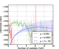
(a) RBM

(b) tDBN-2

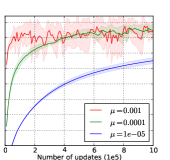
(c) tDBN-3

Figure 1: Sensitivity analysis of the test set likelihood as a function of the learning rate $\mu$. Models considered are (a) a single layer RBM model (b) a 2-layer t-DBN and (c) a 3-layer t-DBN. Shaded areas represent $\pm$ one standard deviation.

We start our evaluation of Deep Tempering on the “Artificial Modes” dataset first introduced in Desjardins et al. (2010a). The dataset is characterized by five basic $28\times 28$ binary random noise images. Training data is generated online as a mixture model over these five modes, permuting each pixel independently with a mode dependent probability. This dataset is difficult from a sampling perspective, as it combines modes of low probability having large spatial support, and narrow modes with high probability. On the other hand, the structure of the data is relatively simple, allowing us to use models with low capacity and thus measure likelihood exactly during training. Likelihood is reported on a test set of $5$k images.

RBM vs. t-DBN

Figure 1 compares the test-set likelihood curve (during training) of a $10$-hidden unit RBM, vs the likelihood of the first-level RBM in a 2 and 3-layer tempered DBN (t-DBN), with $10$ hidden units per layer. We therefore evaluate DT as a better training/sampling algorithm for RBMs. Gradients were computed by averaging over a small mini-batch of size $5$, kept small so as to prevent models from covering all modes through a large mini-batch of (effectively) stationary particles. To simplify the analysis and given the interesting dynamic between learning and mixing (the mixing rate of a sampler constrains the set of feasible learning rates), we focus our hyper-parameter search to constant learning rates in $\{10^{-3},10^{-4},10^{-5}\}$. Results are averaged over $5$ seeds, with the shaded area representing $\pm\sigma$.

As we can see, the single RBM is unable to learn a meaningful model of the dataset for any setting of the learning rate. SML diverges when using high learning rates and yields an unimpressive score of around $-329.6$ nats when using a learning rate of $10^{-5}$. In contrast, a stack of two RBMs trained via Deep Tempering achieves a score of $-120.4$ nats with a learning rate of $10^{-4}$. Pushing the learning rate further to $10^{-3}$ causes the two layer model to diverge, a fact which seems attenuated by moving to a stack of 3 RBMs, shown in Figure 1c. Cross-model state swaps occurred rather frequently on this dataset, with the best performing t-DBN2 model swapping $32\%$ of the time on average.

PT, CAST vs t-DBN.

DT also compares favorably to state-of-the-art tempering methods. In Desjardins et al. (2010a), Parallel Tempering required around $50$ tempered chains spaced uniformly in the unit interval, to achieve a likelihood of around $-175$ nats. Optimizing the inverse temperature parameters through an adaptive tempering mechanism improved this likelihood to around $-150$ nats, while requiring fewer tempered chains ($20$). Results obtained with the original CAST formulation Salakhutdinov (2010a) (CAST 1:1), using $100$ tempered chains spaced uniformly in the unit interval, are shown in Figure 2a. The model originally performs well but eventually diverges despite AST converging to the proper (log) adaptive weights (given by the log-partition functions at each temperature). Suspecting insufficient replica exchanges between tempered and non-tempered chains (given the large number of temperatures being simulated), we also trained a one layer RBM using a modified version of CAST, where we increase the “coupling ratio”, i.e. the ratio of non-tempered to tempered chains, denoted as CAST 1:X. A ratio of 1:10 led to notable improvements in likelihood, achieving $-139.3$ nats after $10^{6}$ updates. CAST 1:100 achieved a new state-of-the-art for single-layer models: $-110.5$ nats. The reader should keep in mind however that CAST $1:100$ with a mini-batch of size $5$ requires simulating $505$ Markov chains in total, compared to the $10$ Markov chains required by a t-DBN2.

DBN Lower-Bound.

As mentioned in Section 3, DT applied to a stack of RBMs can equivalently be viewed as performing joint-training of a DBN. It is thus interesting to study the effect of DT on the lower-bound of the DBN likelihood, as formulated in (Salakhutdinov and Murray, 2008). The results are shown in Figure 2b. The optimal learning rate achieved a lower-bound of $-94.6$ nats for a 2-layer DBN (shown in green), and $-91.0$ nats for the 3-layer variant (red). One may also wonder about the effect of joint-training vs. the typical greedy layer-wise training procedure employed by DBNs. To avoid the extreme instability of SML trained RBMs on this dataset, we adjusted the greedy layer-wise training to incorporate early-stopping, based on detecting oscillations in training likelihood. $M-1$ layers were pre-trained in this manner, followed by joint-training across all layers. The results clearly show worse performance for the pre-trained models. This suggests that the greedy layer-wise pre-training scheme of DBNs leads to poor local minima.

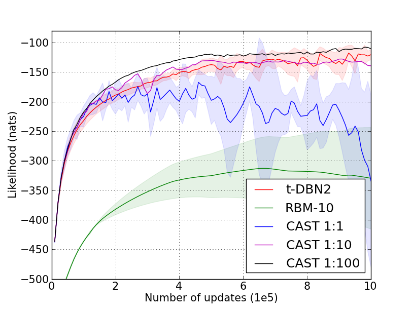
(a)

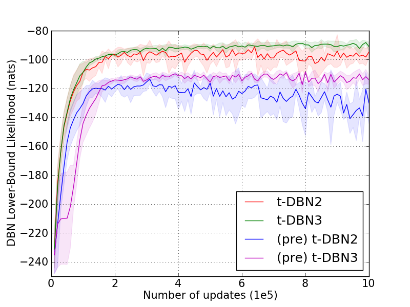
(b)

Figure 2: (left) Likelihood of the first layer RBM for various model configurations / training algorithms. RBM-10 was selected as the best single-layer model from those of Figure 1a, t-DBN2 from Figures (1b, 1c). CAST 1:X shows the likelihood of an RBM trained with Coupled Adaptive Simulated Tempering, having a ratio of non-tempered to tempered chains of 1/X. (right) DBN likelihood lower-bound for the best 2 and 3 layer t-DBNs (joint-trained only, 2 top curves) vs. t-DBNs having first been pre-trained before the joint-training procedure (2 bottom curves).

5 Discussion

Deep Tempering combines ideas from traditional MCMC tempering methods, with new observations from the field of deep learning. From the field of MCMC, we borrow the idea of simulating an ensemble of distributions, where the fast-mixing properties of high-temperature chains is leveraged to facilitate training of the lower layers, which are often prone to getting stuck in regions of high probability. From the world of deep learning, we exploit recent findings which show that models at deeper layers in the hierarchy seem to naturally exhibit good mixing. These two ideas are combined through a joint-training strategy, which considers individual models in a deep hierarchy as interpolating distributions for the lower layers. While we have concentrated on the application of Deep Tempering to RBMs the method is much more widely applicable. Perhaps most interesting is that it can be readily applied to Deep Boltzmann Machines (DBM) Salakhutdinov and Hinton (2009) both to promote mixing in the negative phase of learning as well as to draw diverse samples from a fully trained model. We simply construct a latent variable model over all the even layers of the DBM and use this model to propose swaps with the DBM state over the even layers of the model.

The method that we describe in this paper can be considered an example of an auxiliary variable method Markov Chain Monte Carlo sampling of the lower layer RBM. Similar to other such methods, including the celebrated Sweden-Wang method Swendsen and Wang (1987), one can interpret the addition of the random variables in the upper-layer RBMs (both visibles and hiddens) as auxiliary variables that are added to augment the simulated system with the goal of achieving more efficient sampling. Where the proposed approach differs from more standard auxiliary variable methods for MCMC is the richness in structure relating these auxiliary variables both to themselves and to the target lower-layer RBM. While Swendsen-Wang can be thought of as imposing a clustering on the variables of the simulated system, our approach uses a DBN (with $M-1$ layers) to model the dependency structures between the latent variables of the lower-layer RBM.

References

- Bengio et al. (2013) Bengio, Y., Mesnil, G., Dauphin, Y., and Rifai, S. (2013). Better mixing via deep representations. In ICML’13.
- Cho et al. (2010) Cho, K., Raiko, T., and Ilin, A. (2010). Parallel tempering is efficient for learning restricted Boltzmann machines. In Proceedings of the International Joint Conference on Neural Networks (IJCNN 2010), Barcelona, Spain.
- Desjardins et al. (2010a) Desjardins, G., Courville, A., and Bengio, Y. (2010a). Adaptive parallel tempering for stochastic maximum likelihood learning of rbms. Deep Learning and Unsupervised Feature Learning Workshop, NIPS.
- Desjardins et al. (2010b) Desjardins, G., Courville, A., and Bengio, Y. (2010b). Tempered Markov chain Monte Carlo for training of restricted Boltzmann machine. In JMLR W&CP: Proceedings of the Thirteenth International Conference on Artificial Intelligence and Statistics (AISTATS 2010), volume 9, pages 145–152.
- Hinton et al. (2006) Hinton, G. E., Osindero, S., and Teh, Y. (2006). A fast learning algorithm for deep belief nets. Neural Computation, 18, 1527–1554.
- Luo et al. (2013) Luo, H., Carrier, P. L., Courville, A., and Bengio, Y. (2013). Texture modeling with convolutional spike-and-slab RBMs and deep extensions. In AISTATS’2013.
- Salakhutdinov (2010a) Salakhutdinov, R. (2010a). Learning deep Boltzmann machines using adaptive MCMC. In L. Bottou and M. Littman, editors, Proceedings of the Twenty-seventh International Conference on Machine Learning (ICML-10), volume 1, pages 943–950. ACM.
- Salakhutdinov (2010b) Salakhutdinov, R. (2010b). Learning in Markov random fields using tempered transitions. In NIPS’09.
- Salakhutdinov and Hinton (2009) Salakhutdinov, R. and Hinton, G. (2009). Deep Boltzmann machines. In Proceedings of the International Conference on Artificial Intelligence and Statistics, volume 5, pages 448–455.
- Salakhutdinov and Murray (2008) Salakhutdinov, R. and Murray, I. (2008). On the quantitative analysis of deep belief networks. In W. W. Cohen, A. McCallum, and S. T. Roweis, editors, ICML 2008, volume 25, pages 872–879. ACM.
- Smolensky (1986) Smolensky, P. (1986). Information processing in dynamical systems: Foundations of harmony theory. In D. E. Rumelhart and J. L. McClelland, editors, Parallel Distributed Processing, volume 1, chapter 6, pages 194–281. MIT Press, Cambridge.
- Swendsen and Wang (1987) Swendsen, R. H. and Wang, J.-S. (1987). Nonuniversal critical dynamics in monte carlo simulations. Physical review letters, 58(2), 86.
- Tieleman (2008) Tieleman, T. (2008). Training restricted Boltzmann machines using approximations to the likelihood gradient. In ICML’2008, pages 1064–1071.
- Younes (1999) Younes, L. (1999). On the convergence of Markovian stochastic algorithms with rapidly decreasing ergodicity rates. Stochastics and Stochastic Reports, 65(3), 177–228.