Classical mechanics of economic networks

Abstract

Financial networks are dynamic. To assess their systemic importance to the world-wide economic network and avert losses we need models that take the time variations of the links and nodes into account. Using the methodology of classical mechanics and Laplacian determinism we develop a model that can predict the response of the financial network to a shock. We also propose a way of measuring the systemic importance of the banks, which we call BankRank. Using European Bank Authority 2011 stress test exposure data, we apply our model to the bipartite network connecting the largest institutional debt holders of the troubled European countries (Greece, Italy, Portugal, Spain, and Ireland). From simulating our model we can determine whether a network is in a “stable” state in which shocks do not cause major losses, or a “unstable” state in which devastating damages occur. Fitting the parameters of the model, which play the role of physical coupling constants, to Eurozone crisis data shows that before the Eurozone crisis the system was mostly in a “stable” regime, and that during the crisis it transitioned into an “unstable” regime. The numerical solutions produced by our model match closely the actual time-line of events of the crisis. We also find that, while the largest holders are usually more important, in the unstable regime smaller holders also exhibit systemic importance. Our model also proves useful for determining the vulnerability of banks and assets to shocks. This suggests that our model may be a useful tool for simulating the response dynamics of shared portfolio networks.

Significance

We propose a simple yet powerful deterministic model for a fully dynamical bipartite network of banks and assets and apply it to the Eurozone sovereign debt crisis. The results closely match real-world events (e.g., the high risk of Greek sovereign bonds and the failure of Greek banks). The model can be used to conduct “systemic stress tests” to determine the vulnerability of banks and assets in time-dependent networks. It also provides a simple way of assessing the stability of a system by using the ratio of the log returns of sovereign bonds and the stocks of major holders. We also propose a “systemic importance” ranking, BankRank, for these dynamic bipartite networks.

Recent financial crises have motivated the scientific community to seek new interdisciplinary approaches to modeling the dynamics of global economic systems. Many of the existing economic models assume a mean-field approach, and although they do include noise and fluctuations, the detailed structure of the economic network is generally not taken into account. Over the past decade there has been heightened interest in analyzing the “pathways of financial contagion.” The seminal papers were by Allen and Gale [1, 2] and these were following by many other studies [3, 4, 5, 6, 7, 8]. Economists have recently become aware that econometrics has traditionally paid insufficient attention to two factors: (i) the structure of economic networks and (ii) their dynamics. Studies indicate that a more thorough approach to the examination of economic systems must necessarily take network structure into consideration [9, 10, 11, 12, 13, 14, 15, 16].

One example of this approach is the work of Battiston et al. [17]. They study the 2008 banking crisis and use network analysis to develop a measure of bank importance. By defining a dynamic centrality measurement called DebtRank that measures interbank lending relationships and their importance in propagating network distress, they show that the banks that must be rescued if a crash is to be avoided (those that are “too big too fail”) are the ones that are more “central” in terms of their DebtRank.

Another recent event that has motivated and provided the focus for our study reported here is the 2011 European Sovereign Debt Crisis. It began in 2010 when the yield on the Greek sovereign debt started to diverge from the sovereign debt yield of other European countries, and this led to a Greek government bailout [18]. The nature of the sovereign debt crisis and resulting network behavior that we analyze here differs somewhat from that of the US banking crisis. Here we focus on the funds that several Eurozone countries—Greece, Italy, Ireland, Portugal, and Spain (GIIPS)—had borrowed from the banking system through the issuing of bonds. When these governments faced fiscal difficulties, the banks holding their sovereign debt faced a dilemma: should they divest some of their holdings at reduced values or should they wait out the crisis. The bank/sovereign-debt network that we analyze in this study is a bilayer network. Although DebtRank has also been used to study bipartite networks, e.g., to describe the lending relationships between banks and firms in Japan [19], it does not take into account that link weights exhibit a dynamic behavior.

Huang et al. [20] and Caccioli et al. [21] analyzed a similar problem, that of cascading failure in a bipartite network of banks vs assets in which risk propagates among banks through overlapping portfolios (see also Ref. [22]). Although network connections in real-world financial systems, e.g., interbank lending networks or stock markets, are dynamic, neither of the above models [20, 21] take this into account. Other models by Hałaj and Kok [23], which use simulated networks similar to real systems, or by Battiston et al. [24] allow the nodes to be dynamic but not the links (see, however, Ref. [25], in which dynamic behavior occurs when a financial network attempts to optimize “risk adjusted” assets [26]). Our approach differs from both of these because by introducing only two parameters which play the role of coupling constants in physics we can enable all network variables to be dynamic. Our model is related to Caccioli et al. [21] and Battiston et al. [17] but differs in that we allow both nodes and links to be dynamic.

We use a time-slice of the GIIPS sovereign debt holders network from the end of 2011 to focus on a simplified version of the network structure and use it to set the initial conditions for our model.

We start by proposing, solely on phenomenological grounds, a set of dynamical equations. Based on our analysis we observe that:

1. When we model how a system responds to an individual bank experiencing a shock, our analysis is in accordance with real-world results, e.g., in our simulations Greek debt is clearly the most vulnerable.

2. The dynamics arising from our model produces different end states for the system depending on the values of the parameters.

In order to determine which banks play a systemically dominant role in this bipartite network, we adjust the equity of each bank until it goes bankrupt and then quantify the impact (the BankRank) of the bank’s failure on the system. We simulate the dynamics for different parameter values and observe that the system exhibits at least two distinctive phases, one in which a new equilibrium is reached without much damage and one in which the monetary damage is quite significant, even devastating.

1 The GIIPS problem

Governments borrow money by issuing sovereign (national) bonds that trade in a bond market (which is similar to a stock market).

Our GIIPS data are from the 137 banks, investment funds, and insurance companies that were the top holders in the GIIPS sovereign bond-holder network in 2011. (Hereafter we will use “banks” to refer to all these financial institutions.) Table 1 shows the percentages of the sovereign bonds issued by each GIIPS country owned by these banks. Since our model requires knowing the equity of each bank, we reduce our dataset to the 121 banks whose equity value was obtainable. By the end of 2011, two important Greek banks—the National Bank of Greece and Piraeus Bank—had negative equities. Because our model only considers banks that can execute trades based on positive capital, we also had to eliminate these two banks from our analysis. Figure 1 shows the weighted adjacency matrix of this network.

Table 1: Total amount of exposure of the banks in our data set to the sovereign debt of the GIIPS countries

	Greece	Italy	Portugal	Spain	Ireland
Total (bnEu)	64.85	330.38	30.63	151.15	18.41
% in Banks	23.67	20.13	23.81	21.81	20.55

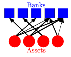
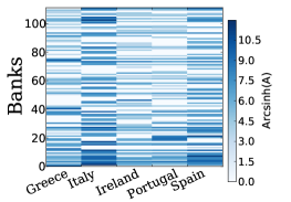
Figure 1: (Left) A sketch of the network of banks vs assets. It is a directed, weighted bipartite graph. The thicknesses represent holding weights. Motion along the edges from banks to assets is described with the wighted adjacency matrix $A$ and the opposite direction, assets to banks, is described with $A^{T}$. (Right) $\sinh^{-1}(A)$ with $A$ being the weighted adjacency matrix of the GIIPS holdings, (weighted by amount of banks’ holdings in GIIPS sovereign debt expressed in units of millions of Euros. The vertical axis denotes different banks (121 of them) and they are ordered in terms of their total exposures to GIIPS debt (higher exposure is at the bottom of the plot) Because holdings differ by orders of magnitude we have plotted $\sinh^{-1}A$ here.

When a country defaults on sovereign debt (or stops paying interest as it comes due) the consequences are usually grave. To prevent cascading sovereign defaults, the European Union, the European Central Bank, and the International Monetary Fund jointly established financial programs to provide funding to troubled European countries. Funding was conditional on implementing austerity measures and stabilizing the financial system in order to promote growth and increase productivity. We use our sovereign debt data as the initial condition for a model of cascading distress propagating through a bipartite bank network in which banks only affect each other through shared portfolios. In order to develop a framework for analyzing these problems that goes beyond simply determining how distress propagates through the links, we construct a model in which dynamic change affects both the weights of links and the attributes of nodes. Figure 1 shows the weighted adjacency matrix of this network in log format.

2 Model

The system that we study is a bipartite network as shown in Fig. 1. On one side we have the GIIPS sovereign bonds, which we call “assets,” and on the other we have the “banks” that own the GIIPS bonds. The nodes on the “asset” side are labeled using Greek indices $\mu,\nu...$. To each asset $\mu$ we assign a “price,” $p_{\mu}(t)$ at time $t$. The “bank” nodes are labeled using Roman indices $i,j...$. Each bank node has an “equity” $E_{i}(t)$, a time $t$, and an initial value of asset $\mu$. Each bank in the network can have differing amounts of holdings in each of the asset types. The amount of asset $\mu$ that bank $i$ holds is denoted by $A_{i\mu}(t)$, which is essentially an entry of the weighted adjacency matrix $A$ of the network. In our model we begin with a set of phenomenological equations describing how each of the variables $E_{i}(t),A_{i\mu}(t)$, and $p_{\mu}(t)$ evolve over time. A key feature of our model is that the weights of links $A_{i\mu}$ are time-dependent, and this introduces dynamics into our network.

2.1 Assumptions, simplifications and the GIIPS system

The key assumptions that differentiate our model from other banking system or dynamic network models are:

1. The banks do not exclusively trade with each other. They may trade with an external entity, which may be the European Central Bank (ECB) or other, smaller investors.

2. When there is no change in equity, price, or bond holdings, nothing happens and there is no intrinsic dynamic activity in our financial network.

3. The model describes the short time response of the system and disregards slow, long-term driving forces of the market.

4. We assume the agents in the system will copy each other’s actions, producing the so-called “herding effect.” This is why we assume the “coupling constants” (the free parameters) are the same for all agents.

3 Notations and Definitions

We denote by $A$ the weighted adjacency matrix, the components of which $A_{i\mu}$ are the amount of exposure of bank $i$ to asset $\mu$. The equity $E_{i}$ of a bank is defined as

$$E_{i}=\sum_{\mu}A_{i\mu}p_{\mu}+C_{i}-L_{i}.$$

Here $p_{\mu}$ is the “price ratio” of asset $\mu$ at a given time to its price at $t=0$, $C_{i}$ is the bank’s cash, and $L_{i}$ is bank’s liability. These parameters evolve in time. Bank $i$ will fail if its equity goes to zero,

$$if:\quad E_{i}=0\quad\to\quad\mbox{Bank $i$ fails.}$$

We assume that the liabilities are independent of the part of the market we are considering and are constant. For convenience we define

$$c_{i}\equiv C_{i}-L_{i}.$$

Two other dependent variables that we use are the “bank asset value” $V_{i}\equiv\sum_{\mu}A_{i\mu}p_{\mu}$ and the total GIIPS sovereign bonds on the market $A_{\mu}\equiv\sum_{i}A_{i\mu}$. In our model we assume that $\alpha$ and $\beta$ are constant. Everything else is time-dependent.

3.1 The time evolution of GIIPS holdings and their price

For changes in equity we have

$$\delta E_{i}=\sum_{\mu}\left((\delta A_{i\mu})p_{\mu}+A_{i\mu}\delta p_{\mu}\right)+\delta c_{i}.$$

Here we assume that the cash minus liability changes according to the amount of money earned through the sale of GIIPS holdings,

$$\delta c_{i}=-\sum_{\mu}(\delta A_{i\mu})p_{\mu}+\delta S_{i}(t),$$

where the minus sign indicates that a sale means $\delta A_{i\mu}<0$ and this should add positive cash to the equity of bank $i$. $\delta S_{i}(t)$ is the cash made from transactions outside of the network of $A_{i\mu}$. The first term in $\delta c_{i}$ cancels one term in $\delta E_{i}$ and we get (all at time $t$)

$$\delta E_{i}=\sum_{\mu}A_{i\mu}\delta p_{\mu}+\delta S_{i}(t).$$

In the secondary market for the bonds (where issued bonds are traded in a manner similar to stocks) the prices are primarily determined by supply and demand. We use a simple model for the pricing that should hold as a first-order approximation. We assume the price changes to be

$$\delta p_{\mu}(t+\tau_{A})=\alpha{\delta A_{\mu}(t)\over A_{\mu}(t)}p_{\mu}(t),$$

Here the coupling constant $\alpha$ is essentially the “inverse of the market depth,” i.e. the fraction of sales ($\delta A/A$ required to reduce the price by one unit ($\delta p/p$) is equal to $1/\alpha$. We are assuming that the market is “liquid” meaning that any amount of assets can be sold or bought without a problem. We have defined $\delta p_{\mu}(t)\equiv p_{\mu}(t)-p_{\mu}(t-\delta t)$ is the change in price from the previous step, $\delta A_{\mu}(t)=A_{\mu}(t)-A_{\mu}(t-\delta t)$ the net trading (number of purchases minus sales) of asset $\mu$, and $\tau_{A}$ the “response time of the market.” We choose the same “inverse market depth” for all GIIPS holdings $\mu$, assuming that they belong to the same class of assets. We then define how the GIIPS holdings are sold or bought, i.e., we define $\delta A_{i\mu}$. We also include a “panic factor” $\beta$ that indicates how abruptly distress propagates when a loss is incurred, and a “market sensitivity” factor $\alpha$ that indicates how quickly the price of an asset drops when part of it is sold. These variables are summarized in Table 2.

Table 2: Notation

symbol	denotes
$A_{i\mu}(t)$	Holdings of bank $i$ in asset $\mu$ at time $t$
$p_{\mu}(t)$	Normalized price of asset $\mu$ at time $t$ ($p_{\mu}(0)=1$)
$E_{i}(t)$	Equity of bank $i$ at time $t$.
$\beta$	Banks’ “Panic” factor.
$\alpha$	“Inverse market depth” factor of price to a sale.

We assume that if a bank’s equity shrinks it will start selling GIIPS holdings in order to continue meeting its liability obligations, and that if a bank’s equity shrinks because of asset value deterioration it will sell a fraction of its entire portfolio to ensure meeting those obligations. The amount of GIIPS holdings sold will depend on how panicked the bank is, i.e., on the value of “panic factor” $\beta$. A bank thus determines what fraction of its equity has been lost in the previous step and sells according to

$$\delta A_{i\mu}(t+\tau_{B})=\beta{\delta E_{i}(t)\over E_{i}(t)}A_{i\mu}(t),$$

where $\tau_{B}$ is the “response time of the banks.” Here we assume that banks purchase using the same protocol as when selling and sell the same fraction of all their GIIPS assets. The above equations can be converted to differential equations by simply replacing $\delta F\to dF/dt$. If we assume that the time lags are small, we can expand the equations with $\tau_{A},\tau_{B}$ to first-order and get

$${dF(t+\tau)\over dt}\approx{d\over dt}\left(F(t)+\tau{dF\over dt}\right)$$

For brevity, we define $\partial_{t}\equiv{d\over dt}$. The three equations become:

$$\left(\tau_{B}\partial_{t}^{2}+\partial_{t}\right)A_{i\mu}(t) =\beta{\partial_{t}E_{i}(t)\over E_{i}(t)}A_{i\mu}(t)$$ (1)

$$\left(\tau_{A}\partial_{t}^{2}+\partial_{t}\right)p_{\mu}(t) =\alpha{\partial_{t}A_{\mu}(t)\over A_{\mu}(t)}p_{\mu}(t)$$ (2)

$$\partial_{t}E_{i}(t) =\sum_{\mu}A_{i\mu}(t)\partial_{t}p_{\mu}(t)+f_{i}(t).$$ (3)

where $f_{i}=dS_{i}/dt$ has the meaning of external force. where $\tau_{B}$ is the time-scale in which Banks respond to the change, and $\tau_{A}$ is the time-scale of market’s response.

In our simulations we use these differential equations and choose $\tau_{A}=\tau_{B}=1$. One of them can always be chosen as a time unit and set to one, but setting them equal is an assumption and may not be true in reality. Our analysis showed that the choice of $\tau_{A,B}$ does not affect the stability of the system and that the stability only depends on $\alpha$, $\beta$ and the shock. The $f_{i}(t)$, which are changes in the equity from what banks own outside of this network, can be thought of as external noise or driving force. We use $f_{i}(t)$ to shock the banks and make them go bankrupt. We shock a single bank, say bank $j$, at a time by reducing its equity 10% by putting $f_{i}(t)=sE_{j}\delta_{ij}\delta(t)$. Starting with $\partial_{t}p_{\mu}(-\varepsilon)=\partial_{t}A_{i\mu}(-\varepsilon)=0$, plugging $\partial_{t}E_{i}$ into (1) and integrating over a small interval $t\in[-\varepsilon,+\varepsilon]$ yields

$$\partial_{t}A_{i\mu}(+\varepsilon) \approx\beta A_{i\mu}(0)\ln(1+s)$$ (4)

This and $E_{i}(\varepsilon)=(1+s)E_{i}(0)$ are the initial conditions we start with. In addition, we require $E,A,p\geq 0$ during the simulations.

4 Application to European Sovereign Debt Crisis

We apply our model to the GIIPS data mentioned above. Before looking at the simulations of Eqs. (1)–(3), we estimate the values of our parameters in the case of the GIIPS sovereign debt crisis.

4.1 Estimating values of $\gamma=\alpha\beta$

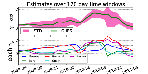
Figure 2: Estimates of $\gamma=\alpha\beta$ over 4 months periods. Top: the shaded purple region is the error-bars based standard deviation and the solid lines are the averages of different $\gamma$ calculated for each country. Bottom: Calculation of $\gamma_{\mu}$ for individual countries. The fact that the values for different countries are close to each other is a sign that our assumption of “herding” (i.e. same $\alpha$ and $\beta$ for all GIIPS) is justified and that our model is applicable here. As can be seen, before the height of the crisis $0<|\gamma|<1$ and then it gradually grows. At the height of the crisis $\gamma\approx 2$. After the crisis we see $\gamma$ decrease again to $\gamma<1$. Later we show that at $\gamma<1$ the system rolls into a new equilibrium, but when $\gamma>1$ the asset prices crash. Also note the timeline of bailouts: Greek bailout approved 2010/04 and 2010/09; Irish bailout 2010/10. these explain part of the movements in the lower plot. The following stock tickers were used for each country (only the top 4 holders of each GIIPS for which stock prices were could be obtained from Yahoo! Finance): Greece: NBG, EUROB.AT, TPEIR.AT, ATE.AT; Italy: ISP.MI, UCG.MI, BMPS.MI, BNP.PA; Portugal: BCP.LS, BPI.LS, SAN; Spain: BBVA, SAN; Ireland: BIR.F, AIB.MU, BEN

We use approximate versions of Eqs. (1)–(3) to estimate the product of parameters $\alpha$ and $\beta$ (details of the approximation and the assumptions are discussed in the SI). The distribution of the assets is roughly log-normal, so a small number banks hold a significant portion of each GIIPS country’s debt. Thus using only the equity of the dominant holders and denoting their sum by $E^{*}_{(\mu)}$ for country $\mu$ will give us a good estimate of $\gamma$. We estimate that the response times $\tau_{A},\tau_{B}$ are at most on the order of several days. Thus we will calculate $\gamma=\alpha\beta$ over a period of four months to allow the system to reach its new final state, and we can discard the second-order derivatives. This allows us to write

$$\delta A_{\mu}\approx\beta\sum_{i}{\delta E_{i}\over E_{i}}A_{i\mu}\approx\beta{\delta E^{*}_{(\mu)}\over E^{*}_{(\mu)}}A^{*}_{\mu},$$

where $E^{*}_{(\mu)}$ denotes the equity of the dominant bank for asset $\mu$. Using this approximation we can relate the first two equations,

$${\delta p_{\mu}\over p_{\mu}}\approx\alpha{\delta A^{*}_{\mu}\over A^{*}_{\mu}}\approx\alpha\beta{\delta E^{*}_{(\mu)}\over E^{*}_{(\mu)}}.$$

Thus we can approximate $\gamma$ as

$$\gamma\approx\frac{\delta p_{\mu}/p_{\mu}}{\delta E^{*}_{(\mu)}/E^{*}_{(\mu)}}.$$ (5)

We evaluate $\gamma$ for each country $\mu$. If the values are similar for different $\mu$ values it may indicate that the “herding effect” is a factor. This both supports our model and suggests that it is applicable to this problem. We evaluate $\gamma$ for the time period between early 2009, when the crisis was just beginning, and early 2011, when most government bailouts had either been paid or scheduled.

If we assume that the number of shares issued by our banks were roughly constant over the period in question, the movements in stock prices may be used as a proxy for the changes in the equity of banks. Many of the major movements (or slope changes) in each country’s $\gamma$ values seem to coincide with bailout payment times.

Figure 2 shows the average $\gamma$ values during this period with standard deviation error-bars. The bottom of the figure gives estimates for $\alpha$ and $\beta$ assuming $|\alpha|=|\beta|$. A more detailed plot with individual values of $\gamma$ obtained using each country is also shown in Fig. 2.

Figure 2 shows that before the crisis $0<|\gamma|<1$ and at its height $\gamma>1$. Below we will explore the phase space in terms of different values of $\alpha$ and $\beta$. An important finding is that our model predicts that $\gamma>1$ is an unstable phase in which a negative shock to the equity of any bank will cause most asset prices to fall dramatically to nearly zero. Similarly, a positive shock will cause the formation of bubbles. When $0<\gamma<1$, on the other hand, after a shock the system smoothly transitions into a new equilibrium and, although some banks may fail, no asset prices will fall to zero.

5 Simulations

We find that when values of $\alpha$ and $\beta$ are small, e.g., $|\alpha\beta|<1$, shocking any of the banks in the network will result in the same final state (see Fig. S2). This is a new stable equilibrium. If we shock the system a second time the prices do not change significantly, i.e., less than 0.1%). Figure 3 shows a sample of the time evolution of the asset prices and the equity of the banks that incurred the largest losses.

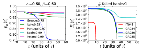
Figure 3: Shocking “Bank of America” with $\alpha=\beta=0.6$. Left: plot of Asset prices over time. Greece incurs the greatest losses, falling to 75% of original value. Final prices are listed in the legend. Right: Equities of the 4 “most vulnerable banks” (2 of major Greek holders incur large losses and one Italian bank is predicted to fail due to the shock). IT043 is Banco Popolare, which has very small equity but large Italian debt holdings. The next two are Agricultural Bank of Greece and EFG Eurobank Ergasias, which are among top 4 Greek holders.

Figure 3 shows results that seem in line with what actually happened during the European debt crisis, although the damage shown for Ireland is less than what actually occurred. In this figure, bailouts are disregarded. Three of the four most vulnerable banks (MVB) shown in Figs. 3 and 4 are holders of Greek debt. In this simulation, Greek debt is the asset that loses the most value. Note that the loss prediction produced by the model is based solely on the network of banks holding GIIPS sovereign debt and provides information about the economies of these countries, with Greece experiencing the largest loss, followed by Portugal (real-world data indicates that Ireland’s loss was as severe as Portugal’s).

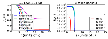
Figure 4: Simulation for larger values of $\alpha$ and $\beta$ (values in legends are final price ratios $p_{\mu}(t_{f})$). This time, in addition to Greek debt, Spanish and Portuguese debt show the next highest level of deterioration. The same four banks are the most vulnerable and this time two more of them fail. At $\alpha=\beta=1.5$ the damages are much more severe than at $\alpha=\beta=0.6$.

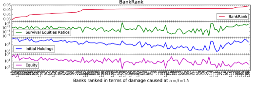
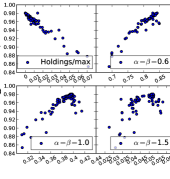
Figure 5: Left: Top: BankRank (6): Ranking the banks in terms of the effect of their failure on the system. Top plot shows the ratio of final total GIIPS holdings in the system to the initial total GIIPS holdings. In this test we do two things. First we increase the equity of the 4 most vulnerable banks up to their total holdings ($E_{i}\to\sum_{\mu}A_{i\mu}$). Then, in each run, we adjust one bank’s equity to just below the minimum equity that would allow it to survive the dynamics (the threshold is found empirically). The initial shock to the system is imposed through shocking the equity of a different bank (not the one we artificially brought to bankruptcy). This way the BankRank tells us how much monetary damage the failing of one bank would cause. The ranking changes slightly for different values of $\alpha$ and $\beta$. At low values, e.g. $\alpha=\beta<1$, the total assets completely determines the ranking. But at larger values, i.e. the “unstable” regime, the correlation reduces significantly. Right: a scatter plot of the BankRank at $\alpha=\beta=0.4$ (vertical axis) versus total holdings over maximum holding (Holding/max), and versus BankRank for other values of parameters at $\alpha=\beta=0.6,1.0,1.5$. BankRank at $\gamma=\alpha\beta<1$ is directly anti-correlated with the initial holdings. BankRank at $\gamma=\alpha\beta>1$ isdifferes significantly from $\alpha=\beta=0.4$, which tells us that in the unstable regime $\gamma>1$ it is no longer true that only the largest holders have the highest systemic importance.

Note that the new equilibrium depends on $\alpha$ and $\beta$. Returning to the real data, Fig. 2 shows that before the onset of the crisis the system responds to a shock by achieving a new equilibrium similar its initial equilibrium (behavior similar to that shown in Fig. 3). At the height of the crisis, however, when $\gamma=\alpha\beta\approx 2$, even a small shock can have a devastating effect and precipitate a crisis (see Fig. 4). Although many banks incur significant losses when $\alpha$ and $\beta$ values are at their highest, the same four banks fail.

In the SI we show the effect of rewiring the banks who lend to each country, meaning we take $A_{i\mu}$ and take random permutations of index $i$ so that the equities of banks connected to each country changes randomly. Interestingly, such a rewiring changes the damages suffered by GIIPS bonds entirely, meaning that Greece will no longer be the most vulnerable. This shows that in our model, while qualitative behavior of the system only depends on $\alpha$ and $\beta$, the final prices and equities depend strongly on the network structure.

6 Systemic Risk and BankRank

We thus take a different approach. We find that a bank can cause a large amount of systemic damage when its equity level is at the bare minimum necessary to survive a shock. Banks with very low equity fail rapidly, no longer trade, and thus no longer transmit damage to the system. Banks with equity sufficient to survive for a significant period of time, on the other hand, continue to transmit damage into the system and thus cause more damage than extremely weak banks. Based on this observation we rank the banks using a “survival equity ratio” (SER), i.e., the fraction of actual equity a bank needs in order to survive systemic shock. The total damage done to the system varies significantly from bank to bank. To rank the systemic importance of each bank we measure the effect their failure has on the system. Since normally no banks other than the four mentioned above fail, we modify the data slightly. The steps we take are as follows:

1. We increase the equity of the four failing banks to $E_{i}(0)=\sum_{i}A_{i\mu}(0)$ to keep them from failing and significantly damaging the system. Then when $\gamma=\alpha\beta<1$, the system becomes resilient to shocks and the drop in prices falls below 1% (the system has reached a stable phase). When $\gamma>1$ the system continues to incur significant losses.

2. To assess the systemic importance of bank $i$, we run separate simulations with initial conditions changed to $E_{i}(0)\in[10^{3}E_{i}(0),10^{-8}E_{i}(0)]$, until we find the threshold of survival under a small shock to any other bank $j$ ($i\neq j$).

3. We calculate the total GIIPS holdings $\sum_{k}(A\cdot p)_{k}$ left in the system.

We define “BankRank” of $i$ to be the ratio of the final holdings to initial holdings if bank $i$ fails, i.e. BankRank of $i$ is equal to the amount of monetary damage the system would take if bank $i$ fails:

$$\mbox{BankRank of~{}}i:R^{i}={\sum_{j}(A\cdot p)_{j}(t_{f})\over\sum_{j}(A\cdot p)_{j}(0)}\Bigg{|}_{\mathrm{Shocking\ }i}.$$ (6)

The smaller the value of $R_{i}$, the greater the systemic importance of bank $i$.

Fig. 5 on the left shows the BankRank in the unstable regime at $\alpha=\beta=1.5$ and how it compares to the initial holdings, minimum ratio of equity required for survival, and initial equities. We observe some correlation between BankRank and each of these variables, but for many banks BankRank does not seem to follow any of these variables. On the right of Fig. 5, on the top left we see that BankRank in the stable regime at $\alpha=\beta=0.4$ has very high correlation with the initial holdings. In the other three plots on the right we see that BankRank changes significantly when we transition from the stable to the unstable regime. This again indicates that, while in the stable regime holding almost completely determine the systemic importance of a bank, in the unstable regime this is no longer the case and many small holders will have high systemic importance.

7 Conclusion and Remarks

We study the systemic importance of large institutional holders of GIIPS sovereign debt and propose a simple, dynamic “systemic risk measurement,” which we call BankRank. We do not find any definitive correlation between BankRank and diversification, but there is a strong correlation between BankRank and total GIIPS holdingsq. Our model describes the response of the GIIPS system to shocks well enough to reveal a “herding effect,” i.e., its presence is indicated whenever a single value for the parameters can be used for the whole system. Our methodology (i) can be used to model “systemic risk propagation” through a bi-partite network of banks and assets, i.e., it can serve as a “systemic stress testing” tool for complex financial systems, and (ii) it can be used to identify the “state” or “phase” in which a financial network resides, i.e., if a banking system is in a fragile state we can quantify it and determine how to transition the system into a more stable state.

We suggest that our model could be useful as a monitoring and simulation tool that allows policy makers to identify systemically important financial institutions and to assess systemic risk build-up in the financial network.

Supporting Information

8 Testing the Role of the Network

Our goal is to determine how much of the above behavior is caused by the network structure and how much by the value of the outstanding debts. To examine the dependence of the results on network structure, i.e., to determine which banks hold which country’s debt and how much bank equities matter, we randomize the network and redo our analysis. We do not change the value of the total GIIPS sovereign debt held by the banks. We only rewire the links in the network, changing the amount of debt held by each bank and the countries to which each bank lends money.

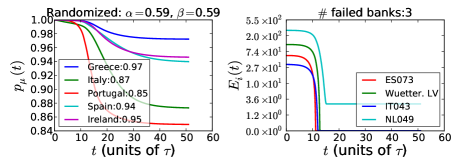
Figure S1: Randomizing which bank lends to which country, while keeping total debt constant for each country. The results differ dramatically from the real world data used in Fig. 3. In this example Portugal and Italy lose the most value, while Greece is the least vulnerable. Other random realizations yield different results.

Figure S1 shows an example of this randomization and how dramatically it changes the end result, and it demonstrates two important features of the model: (i) system dynamics are strongly affected by network structure, i.e., knowing such global variables as the equity and exposure of individual banks is not sufficient, and (ii) real-world data seems to indicate that it was the structure of the network of lenders to Greece that caused Greek sovereign bonds to become the most vulnerable. This suggests that our model may be useful as a stress testing tool for banking networks, or any network of investors with shared portfolios.

9 Shocking different banks

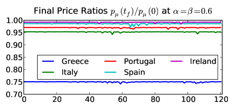
Figure S2: Shocking different banks at $\alpha=\beta=0.6$. The final prices turn out very similar.

Fig. S2 shows the final prices found from shocking different banks. They are all almost identical. However, the small variation and the variations in the $A_{i\mu}(t_{f})$ can be used to construct BankRank and find that different banks have different mounts of influence.

10 The Banks

The listed banks, insurance companies, and funds in the order of largest holders of the GIIPS holdings is given in table 3.

Table 3: GIIPS debt data used in the analysis. All numbers are in million Euros. Our data is based on two sources: 1) The EBA 2011 stress test data, which only includes exposure of European banks and funds (these are the ones where the “Code Name” is of the form CC123); 2) A list of top 50 global banks, insurance companies and funds with largest exposures to GIIPS debt by end of 2011 provided by S. Battiston et al. (These have a name as their “Code Name”), which was consolidated by us.

	Name	Code Name	Holdings	Equity	Greece	Italy	Portugal	Spain	Ireland
0	GESPASTOR	Gespastor	3.5e+02	1.6e+03	0	0	0	3.5e+02	0
1	M&G	M&G	37	1.1e+04	0	0	37	0	0
2	UNION INVESTMENT	Union Inv.	3.4e+03	7e+02	1.6e+02	2e+03	77	1e+03	1.5e+02
3	ATTICA BANK	Attica	1.8e+02	1.5e+04	1.8e+02	0	0	0	0
4	MILANO ASSICURAZIONI	Milano Assic.	74	9.3e+02	23	0	0.71	49	2.1
5	GROUPAMA	Groupama	4.4e+02	4.3e+03	0	4.2e+02	19	0	0
6	AEGON NV	Aegon	1.1e+03	2.6e+04	2	65	9	9.8e+02	26
7	RIVERSOURCE	River Source	48	7.4e+03	48	0	0	0	0
8	AVIVA PLC	Aviva	1.1e+04	1.8e+04	1.5e+02	8.4e+03	2.3e+02	1.4e+03	7.2e+02
9	EMPORIKI BANK	Emporiki	2.9e+02	1.2e+03	2.9e+02	0	0	0	0
10	MELLON GLOBAL	Mellon	16	2.8e+04	0	0	0	0	16
11	DAIWA	Daiwa	7.1e+02	7.3e+03	0	5e+02	0	2e+02	0
12	FIDEURAM	Fideuram	2e+03	5.5e+02	0	2e+03	0	0	0
13	UNIPOL	Unipol	1.3e+04	2.5e+03	26	1.2e+04	1.5e+02	1.1e+03	2.4e+02
14	WGZ BANK AG WESTDT. GENO.	DE029	3.6e+03	1.9e+03	3.2e+02	1.4e+03	4.6e+02	1.2e+03	2.2e+02
15	JYSKE BANK	DK009	1.2e+02	1.4e+04	64	0	19	15	22
16	OESTERREICHISCHE VOLKSBANK AG	AT003	3.7e+02	4.8e+02	1.1e+02	1.5e+02	29	66	13
17	CAIXA PORTUGAL	Caixa (PT)	8.1e+03	2.4e+04	35	4.6e+02	30	7.5e+03	44
18	BLACKROCK	Blackrock	2e+03	2e+04	1.2e+02	1.1e+03	29	7.1e+02	30
19	BANK OF AMERICA	BofA	3.8e+02	1.8e+05	13	2.5e+02	5.4	83	29
20	NORDEA BANK AB (PUBL)	SE084	1.6e+02	2.6e+04	0	97	0	64	1.4
21	CAJA DE AHORROS Y M.P.	ES077	1.5e+03	-	0	0	0	1.5e+03	0
22	SELLA GESTIONI	Sella	6.6e+02	1.3e+02	0	6.6e+02	0	0	0
23	MITSUBISHI UFJ	Mitsubishi	1.6e+03	8.1e+04	0	9.2e+02	71	5.2e+02	62
24	UBS	UBS	1.3e+03	4.8e+04	53	6.8e+02	55	4.4e+02	42
25	OPPENHEIMER	Oppenheimer	2.4e+02	3.8e+02	15	0	0	2.2e+02	0
26	VONTOBEL	Vontobel	18	1.2e+03	18	0	0	0	0
27	NOMURA	Nomura	39	1.8e+04	0	0	20	0	19
28	MACKENZIE	MacKenzie	15	3.4e+03	15	0	0	0	0
29	AGEAS	Ageas	5.3e+03	7.8e+03	6.4e+02	2e+03	1e+03	1.1e+03	5.1e+02
30	DEUTSCHE POSTBANK	De.Postbank	9.2e+02	5.7e+03	9.2e+02	0	0	0	0
31	MORGAN STANLEY	Morgan Sta.	4.6e+02	5e+04	0	4.6e+02	0	0	0
32	HELVETIA HOLDING	Helvetia	1e+03	3.6e+03	7.6	7.2e+02	18	2.4e+02	15
33	HWANG-DBS	Hwang	23	8.7e+02	23	0	0	0	0
34	ASSICURAZIONI GENERALI	Generali	1.7e+04	1.8e+04	1.3e+03	5.4e+03	3.1e+03	5.7e+03	1.7e+03
35	AMLIN PLC	Amlin	15	1.6e+03	0	0	0	15	0
36	SWISS LIFE HOLDING	Swiss Life	5.9e+02	7.5e+03	30	1.7e+02	77	1.8e+02	1.3e+02
37	PHOENIX GROUP	Phoenix	3.2e+02	2.8e+03	0	2.3e+02	11	76	2.2
38	PRICE T ROWE	PT Rowe	15	2.6e+03	0	0	0	0	15
39	AXA	Axa	2.9e+04	4.9e+04	7.6e+02	1.7e+04	1.5e+03	9.4e+03	7.5e+02
40	TOKIO MARINE	Tokio Marine	56	1e+04	0	0	30	0	26
41	ROTHSCHILD	Rothschild	1.1e+02	6e+02	61	0	52	0	0
42	TT ELTA AEDAK	TT Elta Aedak	27	9.3e+02	27	0	0	0	0
43	BALOISE	Baloise	7.9e+02	3.2e+03	84	2.7e+02	98	2.3e+02	1.1e+02
44	NATIXIS	Netaxis	3.3e+03	2.1e+04	4.3e+02	1.3e+03	3.9e+02	8.6e+02	3.9e+02
45	CREDIT AGRICOLE	FR014	1.7e+04	4.9e+04	6.6e+02	1.1e+04	1.2e+03	3.9e+03	1.6e+02
46	JULIUS BAER	Jul. Baer	1.2e+02	3.5e+03	68	0	0	0	57
47	FRANKLIN TEMPLETON	Franklin Temp.	5.1e+03	9.7e+03	0	0	0	0	5.1e+03
48	NOVA LJUBLJANSKA BANKA	SI057	1.7e+02	-	20	96	15	26	15
49	STATE STREET	State St.	51	1.6e+04	0	0	27	0	24
50	ALLIANZ	Allianz	3.8e+04	1e+05	6.2e+02	2.9e+04	7.5e+02	7.1e+03	4.9e+02
51	VIENNA INSURANCE	Vienna	93	5e+03	21	13	0	7	52
52	BANCO POPOLARE - S.C.	IT043	1.2e+04	33	87	1.2e+04	0	2e+02	0
53	COMMERZBANK AG	DE018	2e+04	2.5e+04	3.1e+03	1.2e+04	9.9e+02	4e+03	32
54	LEGAL & GENERAL	L&G	3.8e+02	6.3e+03	1.1	3.3e+02	6.6	35	4.4
55	EFFIBANK	ES063	3e+03	2.7e+03	37	0	16	2.9e+03	0
56	INTESA SANPAOLO S.P.A	IT040	6.2e+04	6.4e+05	6.2e+02	6e+04	73	8.1e+02	1.1e+02
57	IRISH LIFE AND PERMANENT	IE039	1.9e+03	3.5e+03	0	0	0	0	1.9e+03
58	HSBC HOLDINGS PLC	GB089	1.5e+04	1.3e+05	1.3e+03	9.9e+03	1e+03	2e+03	2.9e+02
59	DANSKE BANK	DK008	1.2e+03	1.3e+05	1	5.8e+02	1.1e+02	1.2e+02	4.1e+02
60	ROYAL BANK OF SCOTLAND	GB088	1e+04	9.6e+04	1.2e+03	7e+03	2.9e+02	1.5e+03	4.5e+02
61	BNP PARIBAS	FR013	4.1e+04	8.6e+04	5.2e+03	2.8e+04	2.3e+03	5e+03	6.3e+02
62	BARCLAYS PLC	GB090	2e+04	8e+04	1.9e+02	9.4e+03	1.4e+03	8.8e+03	5.3e+02
63	LLOYDS BANKING GROUP PLC	GB091	94	5.8e+04	0	32	0	62	0
64	DEUTSCHE BANK AG	DE017	1.3e+04	5.5e+04	1.8e+03	7.7e+03	1.8e+02	2.6e+03	5.3e+02
65	SOCIETE GENERALE	FR016	1.8e+04	5.1e+04	2.8e+03	8.8e+03	9e+02	4.8e+03	9.8e+02
66	BPCE	FR015	8.5e+03	4.1e+04	1.3e+03	5.4e+03	3.5e+02	1e+03	3.4e+02
67	BBVA	ES060	6.1e+04	4e+04	1.3e+02	4.2e+03	6.6e+02	5.6e+04	0
68	BANK OF VALLETTA (BOV)	MT046	24	-	10	3.9	2.8	0	7
69	BANCO BPI, SA	PT056	5.5e+03	8.2e+02	3.2e+02	9.7e+02	3.9e+03	0	2.8e+02
70	BANCO SANTANDER S.A.	ES059	5.1e+04	2.6e+04	1.8e+02	7.2e+02	3.7e+03	4.6e+04	0
71	CAIXA DE AFORROS DE GALICIA,	ES067	4.7e+03	2.3e+04	0.0022	1.6e+02	1.3e+02	4.4e+03	0
72	CAIXA D’ESTALVIS DE CATALUNYA	ES066	2.8e+03	2.3e+04	0	0	0	2.8e+03	0
73	CAJA DE AHORROS Y PENSIONES	ES062	3.7e+04	2.2e+04	0	1.3e+03	26	3.5e+04	0
74	KBC BANK	BE005	7.9e+03	1.7e+04	4.4e+02	5.6e+03	1.6e+02	1.4e+03	2.7e+02
75	ERSTE BANK GROUP (EBG)	AT001	1.2e+03	1.5e+04	3.5e+02	6e+02	1e+02	1.4e+02	40
76	JP MORGAN	JPM	17	1.5e+05	0	0	17	0	0
77	BAYERISCHE LANDESBANK	DE021	1.3e+03	1.4e+04	1.5e+02	5.1e+02	1.1e-05	6.6e+02	20
78	BFA-BANKIA	ES061	2.5e+04	1.2e+04	55	0	0	2.5e+04	0
79	SNS BANK NV	NL050	1e+03	5.4e+03	47	7.6e+02	0	57	1.6e+02
80	RAIFFEISEN BANK (RBI)	AT002	4.6e+02	1.1e+04	1.7	4.5e+02	2.1	3.5	0.00016
81	DZ BANK AG DT.	DE020	8.7e+03	1.1e+04	7.3e+02	2.7e+03	1e+03	4.2e+03	51
82	F VAN LANSCHOT	Lanschot	18	7.4e+02	0	0	0	0	18
83	ALLIED IRISH BANKS PLC	IE037	6.5e+03	1.4e+04	40	8.2e+02	2.4e+02	3.3e+02	5e+03
84	SKANDINAVISKA ENSKILDA BANKEN	SE085	6.3e+02	1.2e+04	1.2e+02	2.9e+02	1.3e+02	86	0
85	IBERCAJA	Ibercaja	9.6e+02	2.7e+03	0	0	0	9.6e+02	0
86	LANDESBANK BADEN-WURT…	DE019	2.8e+03	9.5e+03	7.8e+02	1.4e+03	95	5.4e+02	0
87	BANCO POPULAR ESPANOL, S.A.	ES064	9.7e+03	9.1e+03	0	2.1e+02	6.4e+02	8.9e+03	0
88	CAJA ESP. DE INVER. SALAMANCA	ES070	7.6e+03	-	0	0	27	7.6e+03	0
89	NORDDEUTSCHE LANDESBANK	DE022	2.8e+03	6.5e+03	1.5e+02	1.9e+03	2.6e+02	5e+02	41
90	BANCA MARCH, S.A.	ES079	1.5e+02	6.5e+03	0	0	0	1.5e+02	0
91	OP-POHJOLA GROUP	FI012	43	6.2e+03	3.1	0.36	0.00093	0.07	40
92	BANCO COMERCIAL PORTUGUES,	PT054	7.4e+03	4.4e+03	7.3e+02	50	6.5e+03	0	2.1e+02
93	BANCO DE SABADELL, S.A.	ES065	7.4e+03	5.9e+03	0	0	91	7.3e+03	38
94	HYPO REAL ESTATE HOLDING AG,	DE023	1.1e+04	-	0	7.1e+03	4.9e+02	3.4e+03	44
95	FRANKLIN ADVISERS INC	Franklin Adv.	3.6e+02	4.7e+02	0	0	0	0	3.6e+02
96	ABN AMRO BANK NV	NL049	1.5e+03	2.8e+02	0	1.3e+03	0	1.1e+02	1.3e+02
97	MUENCHENER RV	Munich RV	8.2e+03	2.3e+04	5.8e+02	3.6e+03	4.2e+02	1.9e+03	1.8e+03
98	HSH NORDBANK AG, HAMBURG	DE025	1e+03	4.8e+03	1e+02	6.6e+02	62	1.8e+02	0
99	GRUPO BANCA CIVICA	ES071	4.8e+03	-	5.4	0	0	4.7e+03	0
100	CAIXA GERAL DE DEPOSITOS, SA	PT053	6.8e+03	5.3e+03	51	0	6.5e+03	2e+02	23
101	CAJA DE AHORROS DEL MEDITER…	ES083	5.6e+03	3.8e+03	0	20	4.8	5.6e+03	15
102	GRUPO BMN	ES068	3.7e+03	-	0	0	88	3.6e+03	0
103	BANK OF IRELAND	IE038	5.6e+03	1e+04	0	30	0	0	5.6e+03
104	DEKABANK	DE028	6e+02	3.3e+03	87	2.7e+02	32	1.8e+02	30
105	DEXIA	BE004	2.3e+04	3.3e+03	3.5e+03	1.6e+04	1.9e+03	1.5e+03	0.34
106	GRUPO BBK	ES075	3.1e+03	-	0	0	3	3.1e+03	4
107	BANKINTER, S.A.	ES069	3.6e+03	3.1e+03	0	1.2	0	3.6e+03	0
108	WESTLB AG, DUSSELDORF	DE024	2.2e+03	3e+03	3.4e+02	1.1e+03	0	7.5e+02	35
109	UNIONE DI BANCHE ITALIANE SCPA	IT044	1.1e+04	1.1e+04	25	1.1e+04	0	0	0
110	CAJA DE AHORROS Y M.P.	ES072	3.3e+03	2.7e+03	0	3.8e+02	0	2.9e+03	0
111	CAIXA D’ESTALVIS UNIO DE CAIXES	ES076	2.6e+03	-	0	11	0	2.6e+03	13
112	BANK OF CYPRUS PUBLIC CO	CY007	2.8e+03	2.4e+03	2.4e+03	36	0	58	3.2e+02
113	LANDESBANK BERLIN AG	DE027	1.1e+03	2.3e+03	4.5e+02	3.3e+02	0	3.7e+02	0.075
114	ALPHA BANK	GR032	5.5e+03	2e+03	5.5e+03	0	0	0	0
115	UNICREDIT S.P.A	IT041	5.2e+04	9.3e+05	6.7e+02	4.9e+04	94	1.9e+03	58
116	MARFIN POPULAR BANK PUBLIC CO	CY006	3.4e+03	1.7e+03	3.4e+03	0	0	0	39
117	BANCO PASTOR, S.A.	ES074	2.6e+03	1.6e+03	41	1e+02	1.2e+02	2.3e+03	0
118	GRUPO CAJA3	ES078	1.5e+03	-	0	0	0	1.5e+03	8.4
119	TT HELLENIC POSTBANK S.A.	GR035	5.3e+03	9.3e+02	5.3e+03	0	0	0	0
120	EFG EUROBANK ERGASIAS S.A.	GR030	8.9e+03	8.8e+02	8.8e+03	1e+02	0	0	0
121	ESPIRITO SANTO GROUP,	PT055	3.1e+03	6.2e+03	3.1e+02	0	2.7e+03	55	0
122	AGRICULTURAL BANK OF GREECE	GR034	7.9e+03	7.5e+02	7.9e+03	0	0	0	0
123	CAJA DE AHORROS DE VITORIA	ES080	6e+02	-	0	0	0	6e+02	0
124	ING BANK NV	NL047	1.1e+04	3.5e+04	7.5e+02	7.7e+03	7.6e+02	1.9e+03	92
125	RABOBANK NEDERLAND	NL048	1.1e+03	-	3.8e+02	4.4e+02	82	1.6e+02	60
126	WUERTTEMBERGISCHE LV	Wuetter. LV	7.7e+02	1.2e+02	85	4.5e+02	52	1.8e+02	8
127	NYKREDIT	DK011	1.1e+02	-	22	88	0	0	0
128	MONTE DE PIEDAD Y CAJA	ES073	3.3e+03	58	6	3.1e+02	0	2.9e+03	0
129	CAJA DE AHORROS Y M.P.	ES081	6	58	0	0	0	6	0
130	BANCA MONTE DEI PASCHI DI	IT042	3.3e+04	1.9e+03	8.1	3.2e+04	2e+02	2.8e+02	0
131	COLONYA - CAIXA D’ESTALVIS DE	ES082	26	-	0	0	0	26	0
132	BANQUE ET CAISSE D’EPARGNE DE	LU045	2.8e+03	2.9e+03	85	2.4e+03	1.8e+02	1.7e+02	0
133	PIRAEUS BANK GROUP	GR033	8.2e+03	-1.9e+03	8.2e+03	0	0	0	0
134	NATIONAL BANK OF GREECE	GR031	1.9e+04	-4.3e+03	1.9e+04	0	0	0	18
135	ZURICH FINANCIAL	Zurich	8.7e+03	2.5e+04	0	4.2e+03	3.7e+02	3.7e+03	3.7e+02
136	MITSUI	Mitsui	6.4e+02	6.9e+04	0	3.7e+02	25	1.7e+02	76