Fluctuation Spectroscopy: A New Probe of Old Stellar Populations

Abstract

We introduce a new method to determine the relative contributions of different types of stars to the integrated light of nearby early-type galaxies. As is well known, the surface brightness of these galaxies shows pixel-to-pixel fluctuations due to Poisson variations in the number of giant stars. Differential spectroscopy of pixels as a function of fluctuation strength (“fluctuation spectroscopy”) effectively measures the spectral variation of stars as a function of their luminosity, information that is otherwise difficult to obtain for individual stars outside of the Local Group. We apply this technique to the elliptical galaxy NGC 4472, using HST/ACS imaging in six narrow-band ramp filters tuned to spectral features in the range 0.8 $\mu$m – 1.0 $\mu$m. Pixels with $\pm 5$% broad-band variations show differential color variations of 0.1% – 1.0% in the narrow-band filters. These variations are primarily due to the systematic increase in TiO absorption strength with increasing luminosity on the upper giant branch. The data are very well reproduced by the same Conroy & van Dokkum (2012) stellar population synthesis model that is the best fit to the integrated light, with residuals in the range 0.03% – 0.09%. Models with ages or metallicities that are significantly different from the integrated-light values do not yield good fits. We can also rule out several modifications to the underlying model, including the presence of a significant ($>3$ % of the light) population of late M giants. The current observations constitute a powerful test of the expected luminosities and temperatures of metal-rich giants in massive early-type galaxies. Studies of pixels with much larger (negative) fluctuations will provide unique information on main sequence stars and the stellar initial mass function.

1. Introduction

Most of our knowledge of the stellar populations of galaxies comes from fitting stellar population synthesis models to their integrated light, as it is prohibitively difficult to characterize individual stars outside of the local volume. These models are commonly used to measure the total stellar masses of galaxies, as well as their ages, elemental abundances, star formation rates, dust content, stellar initial mass function, and other properties (see the reviews by Walcher et al. 2011; Conroy 2013, and references therein). Many of the model ingredients carry significant uncertainties, which translate into uncertainties in derived stellar population parameters. The uncertainties in derived masses, star formation rates, and other parameters can be $\sim 0.3$ dex or more (see, e.g., Conroy, Gunn, & White 2009; Mitchell et al. 2013).

Figure 1.— Illustration of the pixel-to-pixel variation in the stellar population of an elliptical galaxy. The top panels show the brightness variations in a model elliptical galaxy, based on the light distribution of NGC 4472, as observed with an idealized HST + ACS (with a PSF that is a $\delta$-function). The bottom panels show a bright and a faint pixel in the ACS image, as observed with a hypothetical diffraction-limited 800 m telescope. The insets show color-magnitude diagrams of the stars in these pixels. In faint pixels there is a deficit of luminous giants with respect to the mean, and in bright pixels there is an excess.

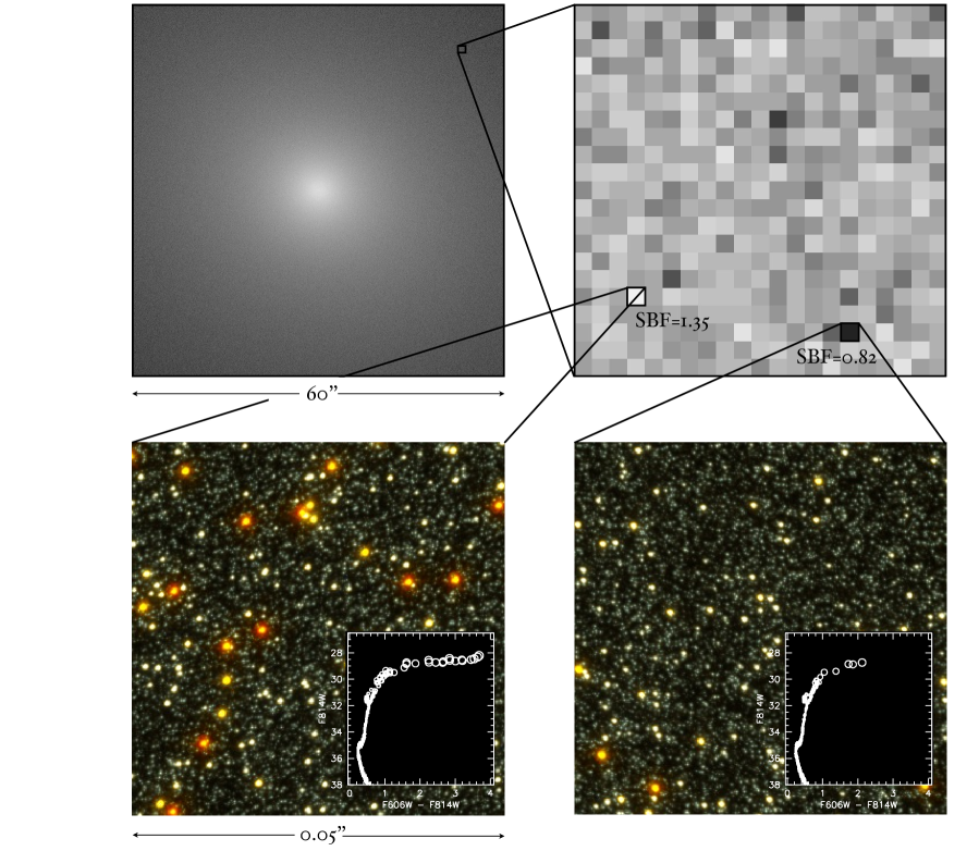
The predictions of stellar population synthesis models have historically been tested with star clusters, as stellar population parameters derived from the integrated light can be compared to those derived from the distribution of stars in the color-magnitude diagram (CMD) (e.g., Worthey 1994; Bruzual & Charlot 2003; Maraston 2005; Schiavon 2007; Conroy et al. 2009; Thomas, Johansson, & Maraston 2011; Noël et al. 2013). In fact, models are frequently tuned and calibrated to fit available data from open clusters in the Milky Way and the Magellanic Clouds, as well as the ancient, and generally metal-poor, globular clusters. Thanks to programs such as the ACS Nearby Galaxy Survey Treasury (ANGST; Dalcanton et al. 2009), some tests can now be done using individual stars in galaxies out to $\sim 4$ Mpc (see, e.g., Girardi et al. 2010).

Despite advances like these, the performance of the models remains essentially untested in important regions of parameter space. Among the most important regimes is that of the metal-rich, old stellar populations which dominate the light of massive early-type galaxies. Correctly modeling these stellar populations is critical for many aspects of astrophysics; examples are the high mass end of the galaxy mass function (Croton et al. 2006) and the core mass function (van Dokkum et al. 2014), the masses of central black holes (van der Marel et al. 1998), the production of atomic elements in the Universe (Worthey, Faber, & Gonzalez 1992; Conroy, Graves, & van Dokkum 2014), the stellar initial mass function (van Dokkum & Conroy 2010; Conroy & van Dokkum 2012b), and the physical conditions in the densest star forming regions in the early Universe (Krumholz 2011; Nelson et al. 2014).

Unfortunately, star clusters in the Local Group with similar ages and abundance patterns as giant ellipticals are rare (e.g., Caldwell et al. 2011; van Dokkum & Conroy 2011). We therefore largely rely on a combination of Milky Way stars and theoretical models to fit the spectra of these galaxies. Of particular concern are the red giants that dominate the near-IR light. The spectra of these stars have strong and ubiquitous molecular bands of titanium-oxide (TiO) and H₂O, which often coincide with spectral features that are used to constrain abundances, ages, and the IMF (see, e.g., Lançon & Wood 2000; Rayner, Cushing, & Vacca 2009).

In this paper we introduce a new method to test the predictions of stellar population synthesis models for old, unresolved stellar populations. The method makes use of the fact that giants are sufficiently rare and luminous that Poisson fluctuations in their number cause pixel-to-pixel fluctuations in the surface brightness distribution of nearby early-type galaxies. The existence of these surface brightness fluctuations is well known, and they have been used extensively to measure distances to galaxies: if a galaxy is closer, there are less giant stars in each pixel, and the pixel-to-pixel Poisson fluctuations around the mean will therefore be larger (e.g., Tonry & Schneider 1988; Tonry et al. 2001; Mei et al. 2005; Blakeslee et al. 2010).

Pixels with high and low fluctuations allow us to do an experiment that gives unique information: we can study how the integrated spectrum changes when giants are added or subtracted to the galaxy. This is illustrated in Fig. 1, which shows the different stellar content of pixels with low and high fluctuations. The bright pixel at bottom left has many more luminous giants than the faint pixel at bottom right; therefore, comparing spectra of pixels with different brightness enables us, in principle, to isolate spectral features of stars on the upper giant branch. Furthermore, in the regime of very large fluctuations there will be pixels (or more appropriately, lines of sight through the galaxy) whose light has only a small contribution from luminous stars on the RGB and AGB. Spectroscopy of these pixels can provide information on the integrated light of stars that are still on the main sequence, which is difficult to access in any other way.

This method builds on previous studies that compared the fluctuation amplitude in various broad-band filters to predictions from stellar population synthesis models (e.g., Worthey 1994; Vazdekis et al. 1997; Blakeslee, Vazdekis, & Ajhar 2001; Liu, Graham, & Charlot 2002; Jensen et al. 2003). A central conceptual difference with previous work is that we do not use the absolute fluctuation signal in the analysis, which is difficult to measure (as it requires an accurate distance, a thorough knowledge of the effects of the PSF, and a careful treatment of contaminating objects). Instead, the method relies on the relative change in the spectrum $\Delta F(\lambda)/\langle F(\lambda)\rangle$ for a given relative change in the total flux $\Delta F/\langle F\rangle$. This is a key strength of the method: the distance, PSF, and other effects that determine the absolute amplitude of the fluctuations are only relevant in that they set the dynamic range that is probed with the data. A second difference is that we identify the fluctuations of individual pixels rather than their statistical ensemble.

Here we take a first step toward fluctuation spectroscopy by using imaging through the narrow-band ramp filters in the Advanced Camera for Surveys (ACS) of HST. We study a regime where the observed fluctuations are dominated by systematic changes in the TiO absorption strength with temperature on the upper giant branch. The target is NGC 4472, the most luminous galaxy in the Virgo cluster (with the possible exception of M87 – depending on the chosen aperture). The main goal of the present paper is to introduce fluctuation spectroscopy as a method to dissect unresolved stellar populations. We also constrain certain aspects of the stellar synthesis model, and we show that more complete tests are possible with future data sets. The paper is organized as follows. In § 2 the HST observations are described, with emphasis on the geometric constraints imposed by the ramp filters. In § 3 the variation in the ramp filters is measured as a function of the variation in the broad-band flux of a pixel. In § 4 we interpret the observed variation in the ramp filters, both in the context of a default isochrone and default population synthesis model and in the context of several variations of this model. The results are summarized in § 6.

2. Data

2.1. Observing Strategy

NGC 4472 was observed for a total of 15 HST orbits in the period Feb 22 – March 1, 2013, in the context of program ID 12523. We used the ramp filters in the ACS camera to obtain images of the galaxy at six different wavelengths. The ramp filters transmit in a narrow optical bandpass, whose central wavelength can be tuned by rotating the filter. Each filter consists of three segments, which are projected on different parts of the WFC detector array. The choice of segment (and therefore the location of the image on the detector) depends on the desired wavelength: within each segment only a limited range of wavelengths can be chosen.

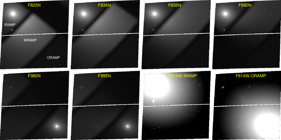
The six filters we used are listed in Table 1. Their transmission curves, calculated with the synphot package, are shown in Fig. 2. The widths of the filters range from $140$ Å for the bluest filter to $200$ Å for the reddest, corresponding to a (sparsely sampled) spectral resolution ranging from $R\approx 58$ to $R\approx 50$. The transmission curves are compared to a model spectrum of an old stellar population (Conroy & van Dokkum 2012a), redshifted to 997 km s^-1 and smoothed to a velocity dispersion of 300 km s^-1. The central wavelengths were chosen to measure three redshifted spectral features that are important indicators of the IMF: the Na I $\lambda 8183,8195$ doublet, the strongest Calcium triplet line Ca II $\lambda 8544$, and the FeH $\lambda 9916$ Wing-Ford band (e.g., van Dokkum & Conroy 2011). For each of these features we observed an “on” band and an “off” band, leading to six narrow-band filters. However, as we show later, the observed pixel-to-pixel variation in these bands in our data is actually not caused by variation in these absorption features, but by systematic changes in the TiO absorption strength on the upper giant branch (see § 4). To avoid confusion we do not refer to these filters as, for example, “Na I on” and “Na I off”, even though that was how they were designed; instead, we use names that simply refer to the central wavelength (see Table 1). Four of the wavelengths fall in the FR853N bandpass, which is part of the inner segment of its ramp filter unit. These images are therefore projected onto the IRAMP aperture, which is in the top left corner of the WFC array. The longest wavelengths fall in the FR1016N bandpass, which is part of the outer segment. The associated ORAMP aperture is in the bottom right corner of the array.

Table 1HST ACS observations of NGC 4472.

Filter	$\lambda_{\rm ramp}$ [Å]	Aperturea	Nameb	Orbits	$t_{\rm exp}$ [s]
FR853N	8230	IRAMP	F823N	2	5237
FR853N	8364	IRAMP	F836N	2	5237
FR853N	8558	IRAMP	F856N	1	2206
FR853N	8796	IRAMP	F880N	1	2164
FR1016N	9802	ORAMP	F980N	2	5237
FR1016N	9951	ORAMP	F995N	3	7636
F814W	—	IRAMP	F814W	2	5237
F814W	—	ORAMP	F814W	2	5237

^a The aperture keyword specifies the pointing origin that is used by HST. Depending on the wavelength, the inner (“IRAMP”) or outer segment (“ORAMP”) of the ramp filter unit has to be used. The galaxy is imaged on opposing corners of the WFC detector array for these two apertures.
^b The name of the filter as it is used in the text.

Figure 2.— Top panel: Model spectrum of a 13 Gyr old stellar population, redshifted to the velocity of NGC 4472 (997 km s^-1) and smoothed to $\sigma=300$ km s^-1. The Na I $\lambda 8183,8195$ doublet, the strongest Ca triplet line Ca II $\lambda 8544$, and the Wing-Ford FeH $\lambda 9916$ band are marked. Bottom panel: The six narrow-band ramp filters that are used in this study. We tuned three filters to the wavelengths of important (redshifted) absorption features, with the other three serving as off-band filters adjacent to the primary filters. As shown in § 4 the observed pixel-to-pixel variation in these six filters is dominated by variation in the strength of TiO.

Figure 3.— ACS images of NGC 4472 in the six ramp filters and in the broad F814W filter. Four of the narrow-band filters require the inner part of the ramp filter structure (“IRAMP”) and two require the outer part (“ORAMP”). A deep, 2-orbit F814W image was obtained for each of these two apertures. The images are scaled to the same exposure time so that differences in brightness indicate differences in S/N ratio. The high S/N F814W images are used to measure the surface brightness fluctuation in each individual pixel.

In addition to the narrow-band data we obtained deep broad-band images of NGC 4472. These broad-band images are critical as they have sufficiently high signal-to-noise ratio (S/N) to accurately measure the flux in each pixel, and therefore the contribution of giants to that pixel relative to its neighboring pixels. The narrow-band data do not have sufficiently high S/N for this measurement, but that is not needed: if it is known which pixels have high fluctuations and which pixels have low fluctuations, we can select the giant-rich and giant-poor pixels in the narrow-band data and average them to increase the S/N ratio. For this to work the broad-band data and narrow-band data have to be astrometrically-matched with an accuracy of $0.1-0.2$ pixel. In order to limit astrometric and resampling errors we observed NGC 4472 twice in the broad-band F814W filter: once using the IRAMP pointing origin and once using the ORAMP pointing origin. This ensures that each narrow-band observation has a matching broad-band observation.

2.2. Image Registration and Matching

Pipeline-processed, drizzled data were obtained from the MAST server. The charge transfer efficiency (CTE) corrected _drc files were used. CTE effects are relatively small in our data as the background is relatively high; nevertheless, the CTE correction removes some faint streaks in the background and produces visibly cleaner images. The data were taken in nine visits: two visits for F995N and one visit for all other bands.

We registered the F823N, F836N, F856N, F880N, and the IRAMP F814W images to a common reference frame. The shifts between these images are small ($\lesssim 10$ pixels), as they all use the same pointing origin. Globular clusters and stars in the field were used to find the shifts; no rotation or scale corrections were needed. We used the F814W image as a reference frame but first shifted it by $\Delta x=0.4$, $\Delta y=0.6$ pixels. This non-integer shift ensures that the broad-band and narrow-band data are interpolated in the same way. We used a third-order polynomial for the interpolation to the reference grid. The F980N, F995N, and ORAMP F814W images were also aligned with each other, using the same procedure. For F995N the two visits were aligned and then added.

The point spread function (PSF) in the images needs to be exactly matched, as any differences will influence the measured signal in the ratio of two bands. We measured the width of the PSF by fitting Gaussians to point sources in the field in each band. It turns out that the width of the F814W PSF is identical (to within $<0.1$ pixel) to the F880N PSF, but that the FWHM of the PSFs in all other bands is narrower by $\approx 0.3$ pixels. It is not clear why the F880N PSF behaves differently from the other ramp filters. We convolved the images to the F814W PSF, and verified that the PSFs were identical to $<0.1$ pixel after the convolution. Images of the eight observations (the six ramp filters and the F814W images in each of the two apertures) are shown in Fig. 3.

Figure 4.— Surface brightness fluctuations in NGC 4472. The left panels show the full F814W images with NGC 4472 centered on the IRAMP (top) and ORAMP (bottom) aperture locations. The middle and right panels show surface brightness fluctuation images at different magnifications. These images were created by dividing the F814W images by smooth models of the galaxy light (see text). The fluctations are not due to noise but due to variations in the number of giants in different sightlines through the galaxy. This is demonstrated by the fact that the fluctuations are identical in the IRAMP and ORAMP images, which are completely independent observations.

3. Analysis

3.1. Modeling of the Smooth Galaxy Light

In order to determine the variation in a pixel we first need to know what the flux in that pixel would be in the absence of fluctuations. We used the deep F814W images to create models for the 2D light distribution of NGC 4472, as imaged at the IRAMP and ORAMP aperture locations. The models were made using the ellipse task in the IRAF STScI package. All parameters were left free in the fit; that is, the ellipticity, center, and boxiness/diskiness of the ellipses were all allowed to vary with radius.

The fits were done in two steps. In the first step, only known bad and missing pixels were masked in the fit. This initial fit was subtracted from the galaxy, and strongly deviating pixels in the residual image ($<-1.5$ or $>1.5$ ADU s^-1) were added to the bad pixel mask. These deviating pixels are mostly at the locations of foreground stars and globular clusters, but also include some bad pixels that were not included in the data quality file. In the second step the fit was improved by adding these flagged pixels to the bad pixel mask.

3.2. Broad-band Fluctuations of Individual Pixels

The surface brightness fluctuation in each pixel was determined in the following way. First, a conservative mask was created that includes all pixels that might be dominated or influenced by globular clusters or stars. In the inner regions of the galaxy these objects were identified by dividing the image by the smooth model, as the relative fluctuations in the center are typically $\lesssim 1$ % (see below). Pixels in the central $\sim 10\arcsec\times 10\arcsec$ that deviate by more than 5 % from the smooth model were identified as potential objects. At larger radii this is not a viable method as the surface brightness fluctuations approach these levels, and we identified contaminating objects by subtracting the model from the galaxy. Away from the central regions, pixels deviating from the model by more than 0.5 counts/s were flagged as potential globular clusters. Careful inspection of the residual images showed that the combined mask correctly identifies all “visible” globular clusters, stars, and background galaxies. The method identifies the central parts of such objects but not their faint wings, and the final mask was created by convolving the combined inner + outer mask with a $9\times 9$ pixel tophat.

After creating the IRAMP and ORAMP masks the F814W images were divided by the smooth 2D models of the light distribution. Pixels flagged in the object masks were set to zero. The resulting residual images contain the surface brightness fluctuations but also low level, large scale variation caused by subtle differences between the surface brightness distribution of the galaxy and the ellipse fit models. This large scale variation was removed using unsharp masking: the residual images were median filtered with a $31\times 31$ pixel mask, and divided by these heavily smoothed versions of themselves. The quantity “surface brightness fluctuation”, or “SBF”, in this paper refers to the fluxes in these residual images. The SBF of a pixel $i$ is therefore defined as SBF = $F_{\rm F814W}^{i}/M_{\rm F814W}^{i}$, with $M$ the flux of a 2D model of NGC 4472 that is constrained to fit the observed F814W surface brightness distribution of the galaxy exactly on $1\farcs 5$ scales.

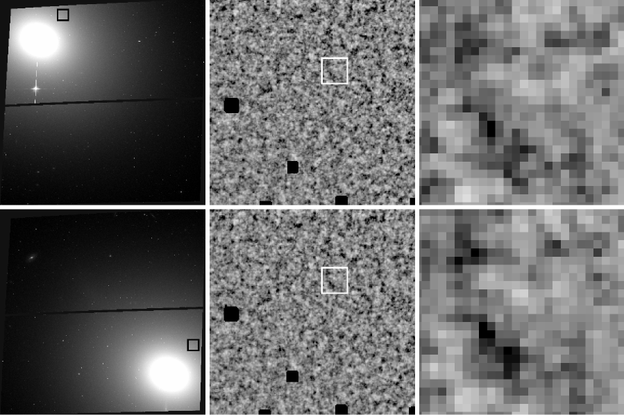
The final surface brightness fluctuation images in the IRAMP and ORAMP apertures are shown in Fig. 4. The images show clear variation, with some pixels being brighter than the mean and others fainter. The reality of the surface brightness fluctuations is demonstrated by their similarity in the top and bottom panels of Fig. 4. The IRAMP and ORAMP observations are entirely independent of each other: the two sets of exposures are independent and the galaxy is exposed on a different detector. Nevertheless, the fluctuation pattern in the IRAMP and ORAMP data is identical, which means that the pattern is dominated by signal, rather than noise.

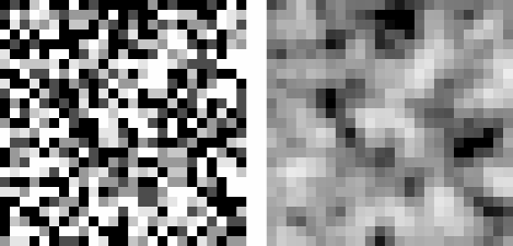
The variation is highly correlated: clumps of pixels vary together. This in itself shows that the pattern is unlikely to be noise, as that is (mostly) uncorrelated in ACS data. The correlations are caused by the HST PSF, which smooths the intrinsically-uncorrelated variations. This is illustrated in Fig. 5, which shows an image with uncorrelated Poisson noise along with the same image convolved with the ACS F814W PSF. The correlated noise pattern is very similar to that seen in Fig. 4. We find that the amplitude of the fluctuations is reduced by a factor of 4.2; that is, in actual ACS images the surface brightness fluctuations are smaller by a factor of $\sim 4$ compared to an imaginary telescope which projects delta functions on a perfect detector with $0\farcs 05\times 0\farcs 05$ pixels. For reference, a Gaussian with a FWHM of 2 pixels reduces the amplitude of random fluctuations by a factor of 3.

Figure 5.— Simulation of the effects of the ACS F814W PSF on the measured fluctuations. The left panel shows a simulated image of uncorrelated Poisson fluctuations. The right panel shows the same image convolved with the F814W PSF. This panel looks similar to the right panels of Fig. 4; the fluctuations are correlated, and their amplitude is reduced by a factor of 4.2 compared to the uncorrelated case.

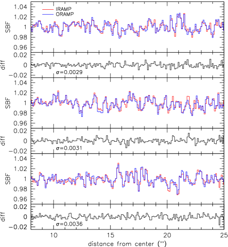
Although the surface brightness fluctuations in the F814W images are dominated by signal, they are not noise-free. We quantify the per-pixel uncertainty empirically by shifting the IRAMP and ORAMP fluctuation images to a common reference frame and subtracting them. The comparison is done after binning the data by a factor of 2 in $x$ and a factor of 4 in $y$, to limit the effects of sub-pixel errors in the shifts. Figure 6 shows three randomly selected 1D traces extracted from the IRAMP and ORAMP F814W fluctuation images. The rms scatter in the difference is 0.003, with no strong dependence on radius in the radial range of interest. Correcting for the binning, and taking into account that the per-image uncertainty is smaller than the uncertainty in the difference of two images by a factor of $\sqrt{2}$, the per-pixel, per-image uncertainty is $0.003\times\sqrt{2\times 4}/\sqrt{2}=0.006$.

Figure 6.— Comparison of F814W surface brightness fluctuations in the independent IRAMP and ORAMP images. Three randomly selected 1D traces are shown, with $2\times 4$ pixel binning. The fluctuations are very similar in the two independent datasets, with an rms difference of 0.3%.

Figure 7.— Left panel: broad-band surface brightness fluctuations in the F814W ORAMP image. Ellipses indicate the galaxy model. Right panel: measured fluctuations in six annuli. As expected, large fluctuations are only found in the annulus that is furthest from the center. Orange lines indicate the expected amplitude of the fluctuations if they scale with $1/\sqrt{F}$.

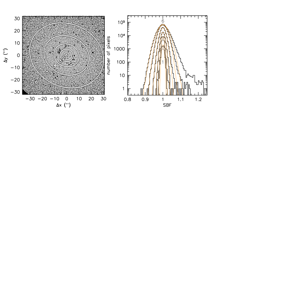
We perform the analysis on relatively small sections of the IRAMP and ORAMP exposures, as the monochromatic patch is $\lesssim 1$ arcmin when the ramp filter assembly is in place. The regions with uniform coverage are approximately $61\arcsec\times 47\arcsec$ and $67\arcsec\times 63\arcsec$ for the IRAMP and ORAMP respectively. The ORAMP monochromatic patch of the F814W surface brightness fluctuation image is shown in the left panel of Fig. 7. The “mottled” appearance is due to the surface brightness fluctuations. The amplitude of the fluctuations increases with distance from the galaxy center. The fluctuations are proportional to $\sqrt{N}$, with $N$ the average number of giant stars in a pixel, which means that the absolute amplitude of the fluctuations is proportional to the square root of the surface brightness. However, the relative fluctuations (which we measure) are proportional to $\sqrt{N}/N=1/\sqrt{N}$, and therefore increase with decreasing surface brightness.

The measured fluctuations in each of six annuli are shown in the right panel of Fig. 7. The rms increases with the distance to the center of the galaxy, from 0.006 in the inner annulus to 0.024 in the outer aperture. The orange curves in Fig. 7 show the expected change with aperture under the assumption that the number of giants is proportional to the surface brightness of the galaxy. This simple expectation fits the observations well (see Tonry & Schneider 1988). The small asymmetry in the observed distributions may be partially caused by faint globular clusters and background galaxies. For the main analysis in the following sections we select all $9\times 10^{5}$ pixels with model surface brightness $\mu_{\rm F814W}<18.8$ mag arcsec^-2.

3.3. Averaged Narrow-band Fluctuations

In contrast to previous studies we are not concerned with an absolute calibration of the surface brightness fluctuation signal. The goal of this study is to measure the spectral variation as a function of the surface brightness fluctuation, that is, to determine by how much the spectrum of a pixel changes for a given change in its brightness. This relative nature of the method is an important aspect, as it makes the analysis independent of the distance of the galaxy, the effects of the PSF, and other effects that determine the amplitude of the fluctuation signal. As discussed earlier, the only requirement is that the PSF and astrometry of the narrow-band observations are matched to those of the broad-band observations.

We measure the spectral variation by dividing adjacent narrow-band filters. Four filter combinations are used: F823N/F836N, F836N/F856N, F856N/F880N, and F980N/F995N. For each of these combinations an “index image” was created by taking the ratio of the two adjacent narrow-band images. These index images were normalized by dividing by the median value of the index. In principle, the images now contain the relative index variation, with respect to a median index value that is identical to 1, for each pixel (in addition to noise). However, the median is not exactly 1 in the entire image, due to relative errors in flat fielding and a possible contribution from real large scale spatial variation in the index. As we are interested only in the relative fluctuations in the indices and not in their absolute values, we divided the index images by a “correction flat” that contains this large scale variation. This correction flat was created by filtering the index images with a median filter of $31\times 31$ pixels. The peak-to-peak variation in the correction flats is $\lesssim 0.1$ %.

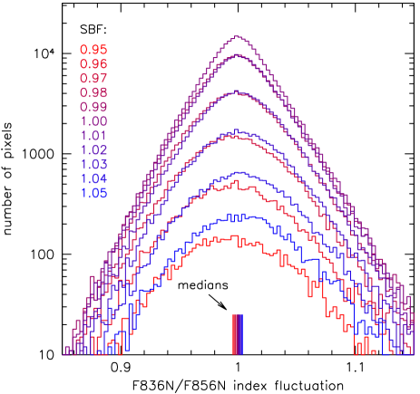
The S/N ratio in the index images is much lower than in the F814W images, due to the much smaller width of the ramp filters. The typical per-pixel measurement uncertainty in the radial range of interest ranges from 0.025 – 0.06, depending on the index. As we will show later, the indices need to be measured with an accuracy of $\sim 0.0005$ to constrain model parameters – two orders of magnitude better than the per-pixel uncertainty. Fortunately, we can obtain the required S/N ratio by binning: as we have a precise measurement of the surface brightness fluctuation of each pixel from the F814W images, we can average all pixels in the index images that are known to have a particular fluctuation. This procedure is demonstrated for the F836N/F856N index in Fig. 8. The rms scatter in individual index measurements (the $1\sigma$ width of the histograms) is $0.031$. Nevertheless, in each surface brightness fluctuation bin the average index value can be determined with an uncertainty of only $\sim 0.0002$ (not including systematic errors), due to the large number of pixels that is averaged. We experimented with different averaging methods and chose the biweight (Beers, Flynn, & Gebhardt 1990), as it is both robust and insensitive to outliers. Using the median instead leads to nearly indistinguishable results. We also explored whether the results depend on the radius from the center of the galaxy, the flat fielding, sky subtraction, and errors in the shifts. The systematic error due to these effects is estimated at 0.0005, that is, 0.05%. This uncertainty was added in quadrature to the Poisson error of each index measurement.

Figure 8.— Index fluctuation measurements, for the N836N/F856N index. The histograms show the measured N836N/F856N index fluctuations in bins of F814W surface brightness fluctuation. The width of these histograms is caused by noise: the $1\sigma$ per-pixel uncertainty is approximately $0.03$. Vertical lines indicate the centers of the distributions of index fluctuations; they range from 0.996 to 1.003, for F814W fluctuations in the range 0.95 – 1.05. These centers (estimated with the biweight, which is very close to a true median) can be determined with an accuracy of $\sim 0.0005$; these are the values that are on the vertical axis of Fig. 9.

Figure 9.— Averaged ramp filter index measurements as a function of surface brightness fluctuation. The four panels show the filter combinations F823N/F836N, F836N/F856N, F856N/F880N, and F980N/F995N. For three of the filter combinations there is a clear relation between the value of the index and the strength of the surface brightness fluctuation. Errorbars are a combination of the expected Poisson noise and a 0.05% contribution from systematic uncertainties. The index values are 1 for SBF = 1 by construction.

The relations between the averaged measured F823N/F836N, F836N/F856N, F856N/F880N, and F980N/F995N indices and the surface brightness fluctuation are shown in Fig. 9. There are clear relations, but the variation is small: over the full range of $\pm 0.05$ fluctuations the indices vary by maximally $\pm 0.002$ for F823N/F836N and F980N/F995N, $\pm 0.004$ for F836N/F856N, and $\pm 0.01$ for F856N/F880N. We note that the relation between the index strength and the surface brightness fluctuation is independent of the spatial resolution of the observations, as long as the quantity on the vertical axis is derived from data with the exact same spatial resolution as the quantity on the horizontal axis. The spatial resolution determines the dynamic range of the fluctuations that are probed at fixed surface brightness, not the form of the correlations between narrow-band indices and the surface brightness fluctuations.

We conclude from Fig. 9 that pixels with high fluctuations have systematically different narrow-band indices than pixels with low fluctuations. In other words, sightlines through NGC 4472 with a relatively high number of giant stars produce a different spectrum than sightlines with a relatively low number of giant stars. The fact that two indices show a positive correlation and one shows a negative correlation implies that we are seeing variation in spectral features, not an overall tilt in the spectrum. In the next Section we interpret the correlations in Fig. 9 in the context of expectations from the stellar spectra that go into the Conroy & van Dokkum (2012a) stellar population synthesis models.

Figure 10.— Spectra of the stars that are used in the Solar metallicity, 13.5 Gyr model. These are the same templates as used in Conroy & van Dokkum (2012a); the spectra are from the IRTF library (Rayner et al. 2009). The most luminous stars have prominent Ca triplet lines as well as strong TiO and H₂O molecular absorption bands. The faintest stars have strong molecular lines, strong Na I and FeH Wing-Ford absorption, and weak Ca triplet lines.

4. Modeling of Fluctuation Spectra

The observed narrow-band index variations are modeled by mimicking the observations as closely as possible. We simulate the stellar population in a pixel by Poisson sampling stars from a stellar library according to an isochrone, and then calculate the total luminosity and the integrated spectrum for each of these pixels. Next, we determine the relations between the narrow-band indices and the surface brightness fluctuations in the same way as was done for the data, taking the redshift and velocity dispersion of the galaxy, the filter curves, and the uncertainties in the data into account.

4.1. Model Ingredients

We use the same empirical stellar spectra that Conroy & van Dokkum (2012a) use in their synthesis of old stellar populations. The number of templates depends on the model age; in our default 13.5 Gyr model 106 templates are used. They are actually 70 distinct stellar spectra, with some of them doing “double duty” in different evolutionary phases that bring them to the same region of the HR diagram. They are carefully vetted Solar metallicity stars from our own Galaxy; their near-IR spectra come from the IRTF spectral library of cool stars (Rayner et al. 2009). Details on their selection and the derivation of their bolometric luminosities and other parameters are given in Conroy & van Dokkum (2012a).

The spectra are shown in Fig. 10. In luminous stars the Ca II triplet lines are strong, whereas Na I and FeH (Wing & Ford 1969) are weak. Low luminosity dwarfs have weak Ca II and prominent Na I and FeH absorption. These characteristics are behind the widespread application of these three spectral features to constrain the stellar mass function from the integrated spectra of old stellar populations (see, e.g., Conroy & van Dokkum 2012b, and references therein). As discussed in § 2 the wavelengths of the ACS ramp filters were chosen to measure the strengths of these (redshifted) features.

In the most luminous and the least luminous stars the spectra show broad bumps and troughs characteristic of molecular transitions. The most prominent of these are H₂O and, particularly, TiO, which has many bands in this wavelength range (Valenti, Piskunov, & Johns-Krull 1998). Two bandheads are marked in Fig. 10. The strength of the H₂O and TiO bands depends on temperature and surface gravity, and they are strongest in late M giants at the tip of the giant branch.

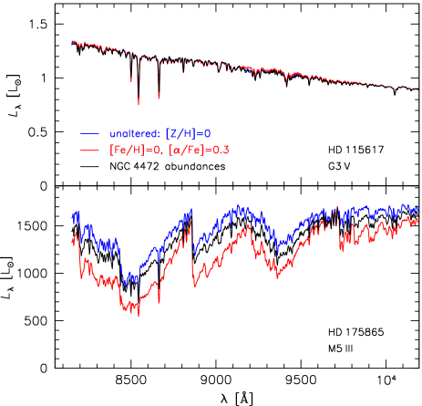
The empirical templates were selected to have Solar abundances, but as is well known elliptical galaxies have non-Solar abundance ratios. In order to explore the effects of metallicity, and to create a default model that resembles NGC 4472 as closely as possible, we have constructed two stellar libraries with alternative elemental abundances. Each individual empirical stellar template was multiplied by the ratio of two theoretical spectra: one with the adjusted abundance, and one with Solar abundance. In this way, the theoretical response to an abundance change is “grafted” onto the empirical spectra. This procedure is similar to that followed in Conroy & van Dokkum (2012a); the difference is that in Conroy & van Dokkum (2012a) we adjusted the integrated spectra and here we apply the corrections to individual stars. The first alternative library comprises “standard” $\alpha$-enhanced spectra, with [Fe/H] = 0 and $[\alpha/$Fe] = 0.3. The second, and default, library is tuned to match the individual elemental abundances of NGC 4472, as derived from integrated-light long-slit spectroscopy (Conroy & van Dokkum 2012a and C. Conroy & P. van Dokkum, in preparation). NGC 4472 has [Fe/H] = 0.05, [Mg/H] = 0.3, [O/H] = 0.3, [Ti/H] = 0.13, [Na/H] = 0.6, [Ca/H] = 0.05, [C/H] = 0.1, and [N/H] = 0.35. In Fig. 11 we show the differences between the spectra of two stars in the three libraries. For Sun-like stars (top panel) the differences are subtle, but for luminous late type giants (bottom panel) they are substantial, with the spectrum that has the NGC 4472 abundance pattern falling in between the (original) Solar-metallicity spectrum and the $\alpha-$enhanced spectrum.

Figure 11.— Abundance variations are accounted for by adjusting the spectra of all individual stars in the library. Two example spectra are shown: a Sun-like star near the main sequence turn-off (top), and a luminous ($L_{\rm bol}\approx 2000L_{\odot}$) red giant (bottom). The original, approximately Solar metallicity spectra are shown in blue. The red and black spectra are created by adjusting the blue spectrum by the theoretical response to changes in the elemental abundances. The red spectra show the effect of increasing the abundance of all $\alpha$-elements. The black spectra (used in our default model) have an abundance pattern that is derived from independent observations of NGC 4472.

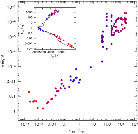
Each star in the library is assigned a weight, which is determined by a combination of a stellar evolution model (as described in Conroy & van Dokkum 2012a) and the IMF. As we did for the metallicity, we base our default model on the best fit to the integrated-light spectrum of NGC 4472 (see Conroy & van Dokkum 2012a). The default weights are therefore calculated for a 13.5 Gyr old stellar population with a Salpeter (1955) IMF. The weight is defined such that it is proportional to the average number of stars in a pixel. The relation between the weight and the bolometric luminosity is shown in Fig. 12. The most luminous giants are rare; only 1 in every 100,000 stars has $L_{\rm bol}>1000\,L_{\rm\odot}$.

Figure 12.— Numerical weight of the stars in the default stellar library, as a function of their bolometric luminosity. This is for a Salpeter IMF and an age of 13.5 Gyr. The points are color-coded by the effective temperature of the stars; the inset shows the location of the stars in the HR diagram. The most luminous giants are rare; there are only a few dozen stars with $L_{\rm bol}>1000L_{\odot}$ in a typical pixel of NGC 4472.

In practice, we simulate $N_{\rm pix}$ “pixels” with a per-pixel mass of $M_{\rm stars}$. For a Salpeter IMF and an age of 13.5 Gyr, the number of stars in each pixel $N_{\rm stars}$ is related to the mass as $N_{\rm stars}=3.4M_{\rm stars}$. We assign $N_{\rm stars}$ to each pixel. Each star in each pixel is labeled with a number from 1 to $n$, with $n$ the number of templates in the library ($n=106$ for the default library). This labeling is based on random numbers, with the probability of assigning a particular template proportional to its weight. The total bolometric luminosity of a pixel is calculated by summing the bolometric luminosities of its stars. We also sum the stellar luminosities integrated over the wavelength range 8150 Å– 8400 Å, as a proxy for the total F814W luminosity. The integrated spectrum of each pixel is constructed by summing the spectra of its stars. Finally, the F814W luminosities were perturbed with a Gaussian of width $0.006\langle L_{\rm F814W}\rangle$, to account for measurement uncertainties in the surface brightness fluctuation measurements (see § 3.2).

4.2. Predicted Surface Brightness Fluctuations

We first compare the distribution of F814W surface brightness fluctuations in our default model to the data. In this comparison, the number of stars per pixel is an adjustable parameter, although we note that our results are not very sensitive to the precise number of stars that is adopted. Figure 13 compares the observed surface brightness fluctuations to those in our default model, for $N_{\rm pix}=2\times 10^{4}$, $N_{\rm stars}=2\times 10^{7}$, and $M_{\rm stars}=6\times 10^{6}$ $M_{\odot}$. For this choice of $N_{\rm stars}$ there is a good match between the distributions, with an rms in both the data and the observations of 0.015. The distributions have a slightly different shape because we did not take the surface brightness profile of NGC 4472 into account in the modeling.

Figure 13.— Comparison of the modeled F814W surface brightness fluctuations (red) to the observed ones (black), for $2\times 10^{7}$ stars per pixel. This model reproduces the width of the observed distribution well. The small difference in the shape of the distribution is caused by the fact that the model does not take the surface brightness profile of NGC 4472 into account.

Figure 14.— Left panel: predicted spectra in the 0.8 $\mu$m – 1.0 $\mu$m range of pixels with SBF = 1.05 (black) and SBF = 0.95 (grey), in our default model. Right panel: predicted fluctuation spectrum, obtained by dividing the two spectra shown in the left panel. The fluctuation spectrum is starkly different from the integrated spectra, and characterized by molecular absorption bands. The thin red line shows a TiO response spectrum (see text) for reference. These TiO and H₂O bands are prominent in red giants with $L_{\rm bol}>1000$ L_⊙.

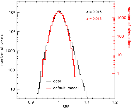
The amplitude of the surface brightness fluctuations is particularly sensitive to the number of giants. As a result, for fixed $N_{\rm stars}$, the model amplitude is a strong function of the IMF, the age, and other parameters. In later Sections we investigate the effects of changing the model parameters, and we always adjust the number of stars per pixel in order to match the observed rms of the F814W surface brightness fluctuations. In this context it should be noted that the parameter $N_{\rm stars}$ is not the true number of stars in a projected $0\farcs 05\times 0\farcs 05$ aperture, but the “effective” number of stars per pixel after smoothing by the ACS PSF (roughly corresponding to uncorrelated areas of $0\farcs 21\times 0\farcs 21$).

We stress that, although we tune the models to reproduce the observed rms, this is actually not necessary. As explained in the Introduction, our method is only sensitive to the relative change in the spectrum for a given relative change in the brightness of a pixel. Specifically, a model with less stars per pixel, and therefore a larger absolute fluctuation signal, produces (to first order) the same relations between spectral variation and flux variation as our default model. The only reason why we adopt a number of stars in the model that produces the correct fluctuation rms is a subtle second-order effect: the smoothing of the modeled F814W luminosities with the observational error (see § 4.1) can only be done correctly if the absolute rms is matched reasonably well.

Although it is not important for our analysis, we can ask whether the observed rms of the fluctuations is similar to the expected rms based on the distance and surface brightness of NGC 4472 and the ACS PSF. Phrased differently, we can ask whether the stellar mass in our model is consistent with the observed surface brightness of NGC 4472. The median surface brightness of NGC 4472 in the analysis region is $\mu_{\rm F814W}=17.7$ mag arcsec^-2. For a distance modulus of $31.17\pm 0.07$ (Mei et al. 2007) this corresponds to $L_{\rm F814W}=(9.5\pm 2.3)\times 10^{5}$ L_⊙ per $(0\farcs 21\pm 0\farcs 02)^{2}$ resolution element. The $M/L_{\rm F814W}$ ratio of NGC 4472, as measured from our Keck LRIS spectrum (Conroy & van Dokkum 2012b, and in preparation), is $3.8\pm 0.5$. The expected stellar mass is therefore $(4\pm 1)\times 10^{6}$ $M_{\odot}$. The stellar mass in our model is a factor 1.5 higher, but the difference is barely significant: based on the surface brightness of NGC 4472 we would have predicted an rms of $0.012\pm 0.002$, and we measure an rms of 0.015.

4.3. Predicted Fluctuation Spectra

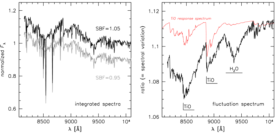
We now turn to the spectral variation as a function of the surface brightness fluctuation. The left panel in Fig. 14 shows the average spectra of simulated pixels with fluctuations of $+5$ % and $-5$ %. The spectra are offset by $\sim 10$ %, as expected, but are otherwise very similar: they are both dominated by the well-known spectral features of old stellar populations (see, e.g., the top panel of Fig. 2).

The right panel shows the ratio of the two spectra, the “fluctuation spectrum”. The fluctuation spectrum is very different from the integrated-light spectra. There are no obvious features at the locations of the Na I $\lambda 8183,8195$ doublet, the Ca II triplet, or the FeH $\lambda 9916$ Wing-Ford band. Instead, the fluctuation spectrum is characterized by sharp bandheads at $\approx 8440$ Å and $\approx 8870$ Å, as well as a broad feature at $\approx 9350$ Å. We identify these features as TiO bandheads and H₂O absorption, respectively. This is demonstrated by the thin red line, which is an approximation of a “pure” TiO spectrum. This TiO spectrum was generated by turning TiO on and off in the modeling of the atmosphere of a single star with $T_{\rm eff}=3750$ K and $\log(g)=1.0$ and then taking the ratio of the resulting spectra.

As can be seen in Fig. 10 the TiO and H₂O bands are strong in the most luminous giants, which have $L_{\rm bol}>1000$ L_⊙ and $T_{\rm eff}=3200$ K – 3600 K. In the regime of small fluctuations, a pixel’s surface brightness fluctuation is essentially determined by the number of these cool, luminous giants it contains. In our default model with $N_{\rm stars}=2\times 10^{7}$ stars per pixel, the average number of stars with $L_{\rm bol}>1000$ L_⊙ per (PSF-convolved) pixel ranges from 91 for pixels with SBF = 0.95 to 150 for pixels with SBF = 1.05.

4.4. Comparison to Observations

We now compare the predicted fluctuation spectra to the observed relations between the narrow-band indices and the F814W surface brightness fluctuations. We averaged the model spectra in each of 11 surface brightness fluctuation bins, from 0.95 to 1.05 with steps of 0.01. The spectra were redshifted to the distance of NGC 4472 (997 km s^-1) and smoothed to a resolution of $\sigma=300$ km s^-1, which is the approximate velocity dispersion of NGC 4472. Then, the spectra were divided by the spectrum of the central surface brightness fluctuation bin, with SBF = 1. This gives 11 differential fluctuation spectra, appropriate for fluctuations ranging from $-0.05$ to $+0.05$. The central fluctuation spectrum is unity at all wavelengths, by construction.

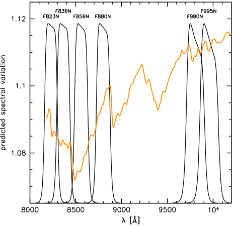
In Fig. 15 we show the ratio of the two extreme spectra, those with SBF = 1.05 and SBF = 0.95. This spectrum can be compared to the unredshifted, unsmoothed version shown in Fig. 14. The six ramp filters are overplotted, after normalizing the filter curves by their peaks. The four blue filters sample wavelengths where there should be significant variation due to TiO, with the two reddest filters effectively acting as a control. The 11 fluctuation spectra were integrated using these synthetic ramp filter curves. Finally, the ratios between adjacent ramp filter fluxes were determined, creating synthetic indices that can be compared to the data.

Figure 15.— Comparison of the ACS ramp filter locations to the predicted spectral fluctuations in our default model. The model was redshifted to the distance of NGC 4472 and smoothed to a velocity dispersion of 300 km s^-1. The four bluest ramp filters sample the strong spectral variation expected from the TiO features in the most luminous giants.

Figure 16.— Comparison of observed ramp filter index variations to predictions from our default model. In the top panels, the points are identical to those in Fig. 9, and the lines are model predictions. The agreement is excellent, which means that we have a good understanding of both the origin of the surface brightness fluctuations and of the spectra of the most luminous giants in massive early-type galaxies. The bottom panels show the residuals from the predicted correlations. The scatter in the residuals is $<0.1$ % in all cases, and lower than the systematic uncertainty of $0.05$ % in three of the four panels. Note that there are no free parameters in the model: the stellar library is that of Conroy & van Dokkum (2012a), and the abundance pattern and age come from a fit to the integrated-light spectrum of NGC 4472.

In Fig. 16 the model predictions are compared to the observed fluctuations in the ramp filters. The data points are the same as those in Fig. 9; the only difference is that the vertical axis spans the same range in all panels of Fig. 16. The lines are predictions from our default model, that is, a model that is based on the stellar library and stellar evolution tracks discussed in Conroy & van Dokkum (2012a), with an age of 13.5 Gyr, the NGC 4472 abundance pattern as measured from its integrated-light spectrum, a Salpeter (1955) IMF, and a stellar mass of $6\times 10^{6}$ $M_{\odot}$ per pixel.

The models provide a remarkably good description of the data, even though they are determined in a completely independent way. Both the sign of the correlations and their amplitude are a close match. The bottom panels of Fig. 16 show the residuals, obtained by subtracting the model predictions from the data. The $1\sigma$ scatter in the residuals is $<0.0005$ for three of the indices. It is slightly higher at $0.0009$ for the reddest index, and there is some evidence for a systematic trend in the residuals for this index. Taking all four indices together, the reduced $\chi^{2}$ is 0.6, which suggests that the systematic error (0.0005) is slightly overestimated. For a systematic error of 0.00025 the reduced $\chi^{2}$ is close to 1.

The excellent correspondence between the observed relations between the ramp filter indices and the F814W surface brightness fluctuations has several implications: it means that we understand the origin of the surface brightness fluctuations in this regime, and also that our stellar population synthesis of the upper RGB and the AGB is correct to within the uncertainties of the method.

Figure 17.— Predicted fluctuation spectra when the underlying stellar population synthesis ingredients are changed. Each panel shows the ratio of the average spectra of pixels with high (SBF = 1.05) and low (SBF = 0.95) fluctuations. The default model (§ 4) is shown in orange. From left to right: model where all giant spectra are replaced with the spectra of main sequence stars of the same effective temperature (§ 5.1.1); model where the spectra of the most luminous giants are switched with those of less luminous giants (§ 5.1.2); effect of changing the number of luminous ($L_{\rm bol}>1000$ L_⊙) stars by a factor of 2 (§ 5.1.3); and the effect of adding a population of very cool giants, contributing 5 % – 15 % of the total luminosity.

5. Effects of Varying Model Parameters

In the previous section we have shown that our default model provides an excellent fit to the observed fluctuations. Here we study the effects of changing various aspects of the model. We consider three distinct types of variation: changes to the underlying model (specifically, the relative weights of stars in the stellar library) (§ 5.1); varying the age, metallicity, and the IMF (§ 5.2); and the regime of very large surface brightness fluctuations (§ 5.3).

5.1. Changes to the Underlying Model

We investigate four variations of the default underlying model. Each model in this section has an age of 13.5 Gyr, the NGC 4472 elemental abundance ratios, and a Salpeter IMF. The variations either change the spectra in the library of 106 templates or change the weights of these templates. Changing the weights effectively means changing the time that stars spend in that particular phase of evolution. The first two of the variations are dramatic (and effectively ruled out by many other observations of stellar populations), and are intended to illustrate the qualitative behavior of the fluctuation spectrum. The last two are more subtle (and more reasonable).

5.1.1 Replacing Giant Spectra by Dwarf Spectra

The first model variation we consider is to ignore the known differences between the spectra of dwarfs and giants and assume that the spectrum of a star depends only on its temperature. We replace the spectrum of every giant in the library by that of the dwarf star whose temperature is closest to that of the giant. As the dwarfs cover a broader range of temperatures than the giants (see the inset of Fig. 12), every giant in the library has a close temperature match on the main sequence. We scale each of the dwarf spectra in such a way that the average brightness in the $0.8\,\mu$m – $1.0\,\mu$m wavelength range is the same as that of the giant it replaces.

The resulting fluctuation spectrum, again obtained by dividing the averaged spectrum of +5 % F814W fluctuations by the averaged spectrum of $-5$ % fluctuations, is shown in the left panel of Fig. 17. The fluctuation spectrum is very different from that of the default model (shown in orange). Cool dwarfs generally have weaker molecular features than cool giants, and we therefore do not see the strong TiO and H₂O bands. Instead, we see that high fluctuations have enhanced Na I and FeH absorption and suppressed Ca II triplet lines, as expected from the spectra of cool dwarfs.

The fluctuation spectra for all 11 surface brightness fluctuation bins were redshifted and smoothed by the velocity dispersion of NGC 4472, just as was done for the default model. We calculated synthetic fluxes in the ramp filters and constructed model indices. In the top panels of Fig. 19 we compared the predictions from this model to the data, and to the default model. The model can clearly be ruled out by the data: the spectra of giants are different from those of dwarfs of the same temperature.

5.1.2 Switching Giants

With this modification we highlight the fact that the most luminous giants, with $L_{\rm bol}>1000$ L_⊙, are responsible for the trends in Fig. 9. We switched the spectra of stars with $L_{\rm bol}>1000$ L_⊙ with those of stars with $L_{\rm bol}=250$ L${}_{\odot}-1000$ L_⊙. No changes were made to stars with $L_{\rm bol}<250$ L_⊙. The rank order within each set of giants was conserved; that is, the brightest star with $L_{\rm bol}>1000$ L_⊙ was switched with the brightest star with $L_{\rm bol}<1000$ L_⊙. As before, we scaled each stellar spectrum so it has the same brightness in the $0.8\,\mu$m – $1.0\,\mu$m range as the star it replaces.

The fluctuation spectrum is shown in the second panel of Fig. 17. Again, the broad molecular features have disappeared, as they now artificially occur in stars that are much more common and therefore do not contribute significantly to the surface brightness fluctuation signal. We now see that the Ca II triplet lines are stronger in pixels with a higher fluctuation. The reason for this behavior is that these lines are very strong in stars with $L_{\rm bol}=250$ L${}_{\odot}-1000$ L_⊙ (see Fig. 10). We will return to this in § 5.3, where we discuss the behavior of the default model in the regime of large, negative fluctuations (that is, SBF $\ll 1$).

In the second row of Fig. 19 the observed ramp filter indices are compared to the predictions from this model. Again, the model is a poor fit: the predicted trends are too weak, due to the absence of strong molecular bands in the fluctuation spectra. As noted earlier, stars with $L>1000$ L_⊙ are rare but contribute significantly to the integrated light. Their treatment is an important source of uncertainty in stellar population synthesis models, and our results provide strong confirmation of the quality of their implementation.

5.1.3 Varying the Contribution of Luminous Giants

Next, we ask what the effect is of changing the contribution of stars with $L_{\rm bol}>1000$ L_⊙ to the total luminosity. This contribution depends on the product of the time spent in their particular phase of evolution and their luminosity. The luminosities are generally better constrained than their timescales, and so we vary the weights of the stars (i.e., how many there are in a pixel) rather than their individual luminosities.

Figure 18.— Spectrum of the M7 giant HD 108849, compared to the average spectrum of stars with $L_{\rm bol}>1000$ L_⊙ in our default library. These stars have spectral types M2 – M6. The M7 star is completely dominated by molecular bands. It has TiO features at the locations of both the Na I $\lambda 8183,8195$ doublet and the Wing-Ford FeH $\lambda{}9916$ band.

The third panel of Fig. 17 shows the effect of increasing (black) and decreasing (grey) the number of luminous giants by a factor of 2. There is an effect on the fluctuation spectrum, with the molecular features becoming stronger for an increasing number of luminous giants, but the effects are small. The reason for this modest change is that the spectral change is, in essence, a second-order effect. To first order, the variation in both the integrated luminosity of pixels and in the normalization of their spectra increases when the number of giants increases. The variation in the spectra at fixed luminosity variation is a more subtle effect.

Figure 19.— Comparison of the observations to the four model variations discussed in § 5.1. Dramatic changes, such as replacing all giant spectra with those of main sequence stars of the same temperature, are very poor fits and can be readily excluded. There is little constraint on the number of giant stars (third row): a factor of 2 change, in either direction, produces nearly identical fits to the data. However, we can rule out a significant additional contribution of very cool giants to the light (bottom row). The lines correspond to contributions of 5 %, 10 %, and 15 % to the light. Even a 5 % contribution to the light produces trends that are too steep, with $\sigma=0.0014$ in the F856N/F880N index.

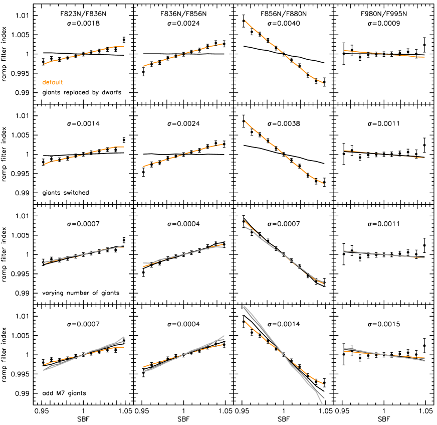
This is also evident in the third row of Fig. 19, where the data are compared to the model predictions. The scatter in the residuals is $<0.001$, and similar to the scatter in the residuals from the default model. The reduced $\chi^{2}$ is 0.6, whereas it is 10.7 and 9.4 for the models considered in § 5.1.1 and § 5.1.2 respectively. To constrain the absolute number of giants an accurate calibration of the absolute surface brightness fluctuation signal is required.

5.1.4 Adding Cool Giant Light

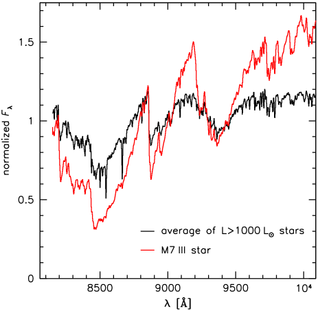
Finally, we consider the possibility that massive elliptical galaxies have a population of very cool giants that is not included in standard stellar population synthesis models at old ages. The strong TiO bands in these stars overlap with several IMF-sensitive features, which is why an arbitrary contribution of M giants is included as one of the nuisance parameters in the Conroy & van Dokkum (2012b) model. The spectrum of such a cool giant is shown in Fig. 18. This M7 III star, HD 108849, has a luminosity $L_{\rm bol}=2150$ L_⊙ and an effective temperature $T_{\rm eff}=3075$ K. It has much stronger molecular bands than the average spectrum of $L>1000$ L_⊙ stars in the default library (which have spectral types M2 – M6).

In the fourth panel of Fig. 17 we show the fluctuation spectrum for a model where we add a population of these cool giants to the light. The weight of this new template is determined by setting the contribution of these stars to the total integrated light in the $0.8\,\mu$m – $1.0\,\mu$m range to 5 %, 10 %, and 15 % (black, dark grey, and light grey in Fig. 17). As might have been expected the fluctuation spectrum shows stronger molecular features than the default model.

Figure 20.— Predicted fluctuation spectra for different ages, metallicities, and IMFs. Each panel shows the ratio of the average spectra of pixels with positive and negative 5 % fluctuations (that is, SBF = 1.05 and SBF = 0.95). The predicted spectra depend on the age and metallicity, but not on the IMF. The default model, shown in orange in all panels, is based on the best fit to the integrated-light spectrum of NGC 4472.

As shown in the bottom row of Fig. 19, even the model with the smallest contribution from M7 giants is clearly a worse fit to the data than the default model. The scatter in the residuals from the fit is 0.0014 for the F856N/F880N index, compared to 0.0004 in the default model. The reduced $\chi^{2}$ is 1.5 for the 5 % model (with 43 degrees of freedom), 3.4 for the 10 % model, and 6.0 for the 15 % model. The 5 % model can be rejected with 98 % confidence, and the other models with $>99$ % confidence.

5.1.5 Summary of Results

From the four modifications that we considered we can infer that the data are sensitive to the spectra of the most luminous giants (those with $L\gtrsim 1000$ L_⊙). This conclusion applies to the regime of small fluctuations (with an rms of 0.01 – 0.02), and the wavelength range 0.8 $\mu$m – 1.0 $\mu$m. The data are remarkably insensitive to the number of these stars, as shown in the third row of Fig. 19. As explained in § 4.3 this is because varying the number of these stars “stretches” the relations between narrow-band indices and the surface brightness fluctuations, but does not change their slope.

Of the four modifications, the first two (§ 5.1.1 and § 5.1.2) mostly serve to illustrate the fact that the fluctuations are only sensitive to the most luminous giants. The latter modifications (§ 5.1.3 and § 5.1.4) are non-trivial and “realistic”, as the lifetimes and temperatures of luminous AGB stars are not well-known from first principles. Perhaps the most directly applicable result is that we can exclude a significant contribution from giants that are cooler than the lowest temperature ones in our default $t=13.5$ Gyr library. The formal upper limit on their contribution is 3 % (with 95 % confidence), although we note that this ignores unknown systematic effects as well as possible degeneracies with other parameters. This constraint can be used in stellar population synthesis models to limit the allowed parameter space (see, e.g., Supp. Fig. 2 in van Dokkum & Conroy 2010 and the discussion in Conroy & van Dokkum 2012b).

5.2. Varying Age, Metallicity, and the IMF

In this Section we fix the underlying components of the model and consider variation in the stellar population parameters age, metallicity, and IMF. In our default model these parameters are taken from the stellar population synthesis model that provides the best fit to the high quality Keck integrated-light spectrum of NGC 4472 (Conroy & van Dokkum 2012a; C. Conroy & P. van Dokkum, in preparation). This fit has an age of 13.5 Gyr, an IMF that is close to Salpeter, and the elemental abundance pattern that is described in § 4.1. As we showed in the previous section, the ramp filter data samples molecular bands in stars on the upper giant branch; even though we use the same underlying model as Conroy & van Dokkum (2012a) it is by no means guaranteed that the best-fitting model to the integrated light spectrum also provides the best fit to the surface brightness fluctuation signal.

Figure 21.— Comparison of the observations to models with varying age, metallicity, and IMF. The ramp filter data are poorly fit with models that are younger than $\sim 11$ Gyr or have a “standard” $\alpha-$enhancement of 0.3. The data provide no constraint on the IMF. Overall the best fits are obtained for the default model (orange in all plots), which was derived from integrated-light spectroscopy.

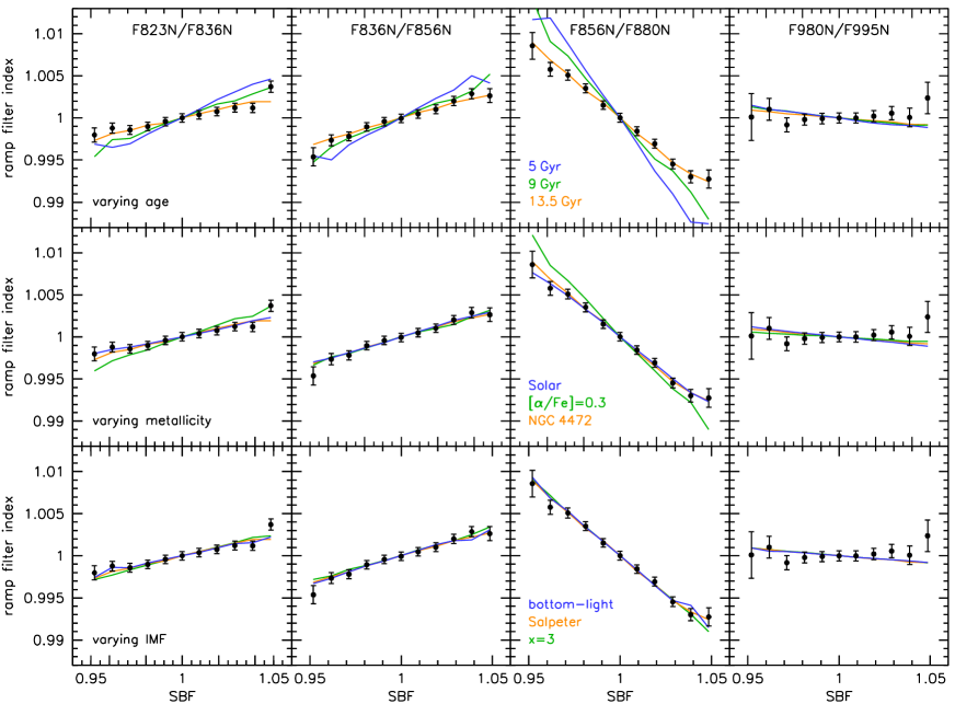
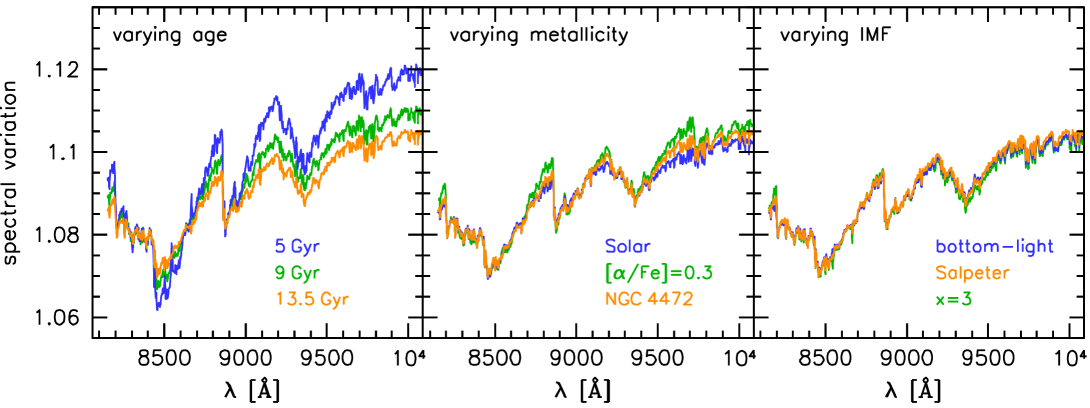
In addition to the default model we consider two younger ages (9 Gyr and 5 Gyr), two alternative abundance patters (Solar and the “standard” $\alpha-$enhanced model described in § 4.1), and two alternative IMFs (a very bottom-heavy IMF with $x=3$, and a bottom-light van Dokkum (2008) IMF with $m_{c}=2$ $M_{\odot}$). The predicted fluctuation spectra are shown in Fig. 20, and the predicted ramp indices are compared to the observations in Fig. 21.

We find that the indices are quite sensitive to age. The 9 Gyr model can formally be excluded at $>99$ % confidence. The reason for this sensitivity is that younger ages have a greater contribution of late M giants. In particular, the number of M6 giants is a factor of $\sim 3$ higher in the 9 Gyr model than in the 13.5 Gyr model. As these late type giants – whose spectra have very strong molecular absorption bands – dominate the surface brightness signal, the change in their contribution at old ages produces a readily detectable signature. The age constraint from the surface brightness fluctuations is fully consistent with the very old age derived from NGC 4472’s integrated-light spectrum, which is mostly sensitive to the properties of stars near the main sequence turn-off. A caveat here is that the measurements are not truly independent, for two reasons: we are using the same model ingredients for both constraints, and late M giants would not contribute solely to the surface brightness signal but also to the integrated light.

The indices are also sensitive to metal abundance, but not in a straightforward way. The standard $\alpha-$enhanced model predicts steeper relations than observed, and can be ruled out with high confidence. However, the predicted trends for Solar metallicity are very similar to those of the default model (and a good fit to the data), despite the fact that the default model has Mg and O abundances that are much closer to the $\alpha-$enhanced model than to the Solar model. As discussed in § 4.1, the only features that really matter are the TiO bands, and the Ti abundance of NGC 4472 is relatively low.

Figure 22.— The regime of large fluctuations. Top left: predicted distribution of surface brightness fluctuations for a Salpeter IMF and $10^{5}$ stars per pixel, a factor of 200 lower than in our HST observations of NGC 4472. Top right: fluctuation spectra in different regimes, from fluctuations $\ll 1$ to fluctuations $\gg 1$. Large positive fluctuations are dominated by luminous RGB and AGB stars. Large negative fluctuations (SBF $<0.9$) probe lower luminosity RGB stars, subgiants, and main sequence stars. Bottom panels: ramp filter index predictions for different IMFs. There is an IMF dependence, particularly for IMFs steeper than the Salpeter form.

The data provide no direct constraint on the IMF. The amplitude of the broad-band fluctuations is sensitive to both the number of stars and the IMF, but we adjust the number of stars so that all models match the observed rms of the broad-band fluctuations. In the regime of small fluctuations the trends in Fig. 21 depend on the luminosity – temperature relation on the upper giant branch, and are independent of the number of low mass stars. Although there is no direct IMF dependence, the results presented in this paper are relevant to measurements of the IMF from integated light, as these rely on accurate modeling of the contribution of luminous giants to the spectra of early-type galaxies.

5.3. Predictions For Large (Negative) Fluctuations

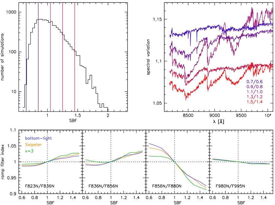
In this paper we focused on a regime of relatively small surface brightness fluctuations, of $\pm 5$ %. This range is dictated by the currently-available data: the Poisson errors quickly increase for fluctuations $<0.95$ and $>1.05$, as we simply do not have many pixels with variations that large. As a result of the small observed fluctuation range there are, on average, $\sim 90$ stars with $L_{\rm bol}>1000$ L_⊙ even in the lowest fluctuation pixels. The fluctuation spectra are therefore completely dominated by the TiO and H₂O features that are characteristic of these luminous red stars.

Here we briefly consider what we can expect in a regime where there are far fewer stars per pixel, so that the surface brightness flucations are much larger. There is a wealth of information in the fluctuation spectra in this regime, as there are sightlines that are free of luminous giants. Those pixels, with surface brightness fluctuations much smaller than 1, provide a window of the lower giant branch and the main sequence that is unattainable in integrated light observations.

We simulated fluctuation spectra in this regime, using our default model with $\langle N_{\rm stars}\rangle=10^{5}$ per pixel rather than $2\times 10^{7}$. In this model there are pixels that contain no stars with $L_{\rm bol}>1000$ L_⊙. The distribution of fluctuations in this model is shown in the top left panel of Fig. 22. The $1\sigma$ spread is $\approx 0.22$ but the distribution is asymmetric, with the high fluctuation tail containing multiple luminous giants. In the top right panel of Fig. 22 we show fluctuation spectra in five regimes, going from surface brightness fluctuations much lower than 1 to fluctuations much greater than 1. The fluctuation spectra are dramatically different in these regimes, as they probe different types of stars. Low fluctuations (0.7/0.6) probe the variation of subgiants and low luminosity giants with temperature, and as these stars have no strong TiO features the fluctuation spectra are dominated by Na I and Ca II. Intermediate fluctuations (1.1/1.0) are predicted to show very strong TiO features in the fluctuation spectra, as the amplitude of their broad-band fluctuation depends on whether they have zero or one star with $L_{\rm bol}>1000$ L_⊙. The regime of strongly positive fluctuations (1.5/1.4) resembles the regime probed in our observations of NGC 4472, that is, the variation of the spectra of very luminous giants with temperature.

The bottom panels of Fig. 22 show the predicted relations between ramp filter indices and the F814W surface brightness fluctuation. The relations are not linear, and they depend on the IMF. Bottom-heavy IMFs with $x=3$ show characteristic asymmetric trends, with little dependence on the surface brightness amplitude for SBF $<$ 1 and steep relations for SBF $>$ 1. Note that the horizontal and vertical ranges of these panels are much larger than in the previous sections.

6. Summary and Conclusions

In this paper we introduced a new technique for studying old, “semi-resolved” stellar populations. We have shown that it is possible to identify individual pixels, or sightlines, in moderately deep HST imaging that have an increased or decreased number of giant stars due to Poisson variations. By averaging carefully matched narrow-band filter observations in bins of surface brightness fluctuation, we have quantified how the spectrum of NGC 4472 changes when giant stars are added or taken away.

The resulting relations between narrow-band indices and broad-band surface brightness fluctuations are remarkably well reproduced with the basic ingredients of the Conroy & van Dokkum (2012a) stellar population synthesis model. The residuals from the predicted relations are very small at 0.03 % – 0.09 %. Qualitatively, this means that the model passes an important test in a previously unexplored regime. It also means that we know what the most luminous stars in elliptical galaxies are: giants with temperatures $T_{\rm eff}\sim 3400$ K and luminosities $L_{\rm bol}\sim 1300$ L_⊙. Their spectra are well understood, even to the extent that our default model with the NGC 4472 abundance pattern is a significantly better match to the data than a “standard” $\alpha-$enhanced model with [$\alpha/$Fe] = 0.3. Understanding stars with $L_{\rm bol}>1000$ L_⊙ is important as they comprise $\approx 17$ % of the bolometric luminosity of old stellar populations, and their strong TiO spectral features coincide with the IMF-sensitive features Na I and FeH. We stress, however, that our data do not provide information on lower luminosity stars, or on the absolute number of luminous giants (see § 5.1.3).

We have tested various perturbations of our default model. The most important result is that we can quantitatively constrain the contribution of late M giants to the integrated light. Such stars are not expected to exist in substantal numbers in old stellar populations, but their presence cannot easily be ruled out based on integrated light analysis. Importantly, leaving the contribution of these stars as a free parameter in fitting stellar populations can lead to degeneracies with the derived stellar initial mass function, as several TiO bands overlap with IMF-sensitive features (see § 5.2 in Conroy & van Dokkum 2012b). Here we show that, for this particular galaxy, they cannot contribute more than 3 % to the integrated light.

Taking the stellar templates and isochrones as a given, we have explored the dependence of the observed ramp filter data on stellar population parameters. In the regime of small fluctuations the data are insensitive to the IMF, but they provide constraints on metallicity and age. In particular, the fluctuation spectra are quite sensitive to age, as the number of late M giants with strong TiO features drops sharply at very old ages. It is generally difficult to distinguish stellar populations that are between 10 and 13 Gyr old, and fluctuation spectroscopy is probably among the most sensitive diagnostics in this regime.

The analysis in this paper can be extended in various directions. The two most obvious ones are to obtain actual spectra rather than narrow-band filter data, and to probe regimes of larger surface brightness fluctuations. As illustrated in Fig. 22 we can expect qualitative changes in the spectra of fluctuations $\ll 1$, as these sightlines offer a relatively unobstructed view of subgiants and the main sequence. The analysis could center on differential techniques such as those employed in this paper, or on direct modeling of the spectra of very negative fluctuations. In principle, it should be possible to empirically, and spectroscopically, reconstruct the entire upper RGB of elliptical galaxies – something that is impossible to do in any other way. Among other applications, this type of analysis should provide strong constraints on the IMF (bottom panel of Fig. 22). Observations with integral-field spectrographs on existing telescopes, particularly when combined with adaptive optics, could provide this kind of information for galaxies within $\sim 3$ Mpc. With JWST and 30m class telescopes on the ground these studies could be extended to the Virgo cluster and beyond.

Progress can also be made by combining constraints from fluctuation spectroscopy with those from fits to integrated-light spectra. The methods provide complementary information, as traditional blue spectra are mostly sensitive to stars near the main sequence turn-off. We note here that none of the model variations discussed in this paper lead to dramatic (that is, larger than a few percent) variations in the integrated-light spectra, with the exception of the models with very young ages. Finally, the stellar library can be augmented. We currently use only 70 distinct templates in our default library, and in some regimes incomplete coverage leads to large “jumps” from one template to the other. Future improvements will be enabled by larger and more comprehensive stellar libraries.

References

- (1) Beers, T. C., Flynn, K., & Gebhardt, K. 1990, AJ, 100, 32
- (2) Blakeslee, J. P., Cantiello, M., Mei, S., Côté, P., Barber DeGraaff, R., Ferrarese, L., Jordán, A., Peng, E. W., et al. 2010, ApJ, 724, 657
- (3) Blakeslee, J. P., Vazdekis, A., & Ajhar, E. A. 2001, MNRAS, 320, 193
- (4) Bruzual, G. & Charlot, S. 2003, MNRAS, 344, 1000
- (5) Caldwell, N., Schiavon, R., Morrison, H., Rose, J. A., & Harding, P. 2011, AJ, 141, 61
- (6) Conroy, C. 2013, ARA&A, 51, 393
- (7) Conroy, C., Graves, G. J., & van Dokkum, P. G. 2014, ApJ, 780, 33
- (8) Conroy, C., Gunn, J. E., & White, M. 2009, ApJ, 699, 486
- (9) Conroy, C. & van Dokkum, P. 2012a, ApJ, 747, 69
- (10) Conroy, C. & van Dokkum, P. G. 2012b, ApJ, 760, 71
- (11) Croton, D. J., Springel, V., White, S. D. M., De Lucia, G., Frenk, C. S., Gao, L., Jenkins, A., Kauffmann, G., et al. 2006, MNRAS, 365, 11
- (12) Dalcanton, J. J., Williams, B. F., Seth, A. C., Dolphin, A., Holtzman, J., Rosema, K., Skillman, E. D., Cole, A., et al. 2009, ApJS, 183, 67
- (13) Girardi, L., Williams, B. F., Gilbert, K. M., Rosenfield, P., Dalcanton, J. J., Marigo, P., Boyer, M. L., Dolphin, A., et al. 2010, ApJ, 724, 1030
- (14) Jensen, J. B., Tonry, J. L., Barris, B. J., Thompson, R. I., Liu, M. C., Rieke, M. J., Ajhar, E. A., & Blakeslee, J. P. 2003, ApJ, 583, 712
- (15) Krumholz, M. R. 2011, ApJ, 743, 110
- (16) Lançon, A. & Wood, P. R. 2000, A&AS, 146, 217
- (17) Liu, M. C., Graham, J. R., & Charlot, S. 2002, ApJ, 564, 216
- (18) Maraston, C. 2005, MNRAS, 362, 799
- (19) Mei, S., Blakeslee, J. P., Tonry, J. L., Jordán, A., Peng, E. W., Côté, P., Ferrarese, L., West, M. J., et al. 2005, ApJ, 625, 121
- (20) Mei, S., Blakeslee, J. P., Côté, P., West, M. J., Ferrarese, L., Jordán, A., Peng, E. W., Anthony, A., & Merritt, D. 2007, ApJ, 655, 144
- (21) Mitchell, P. D., Lacey, C. G., Baugh, C. M., & Cole, S. 2013, MNRAS, 435, 87
- (22) Mould, J. 2012, ApJ, 755, L14
- (23) Nelson, E., van Dokkum, P., Franx, M., Brammer, G., Momcheva, I., Førster Schreiber, N., da Cunha, E., Tacconi, L., et al. 2014, Nature, 513, 394
- (24) Noël, N. E. D., Greggio, L., Renzini, A., Carollo, C. M., & Maraston, C. 2013, ApJ, 772, 58
- (25) Rayner, J. T., Cushing, M. C., & Vacca, W. D. 2009, ApJS, 185, 289
- (26) Salpeter, E. E. 1955, ApJ, 121, 161
- (27) Schiavon, R. P. 2007, ApJS, 171, 146
- (28) Thomas, D., Johansson, J., & Maraston, C. 2011, MNRAS, 412, 2199
- (29) Tonry, J. & Schneider, D. P. 1988, AJ, 96, 807
- (30) Tonry, J. L., Dressler, A., Blakeslee, J. P., Ajhar, E. A., Fletcher, A. B., Luppino, G. A., Metzger, M. R., & Moore, C. B. 2001, ApJ, 546, 681
- (31) Valenti, J. A., Piskunov, N., & Johns-Krull, C. M. 1998, ApJ, 498, 851
- (32) van der Marel, R. P., Cretton, N., de Zeeuw, P. T., & Rix, H.-W. 1998, ApJ, 493, 613
- (33) van Dokkum, P. G. 2008, ApJ, 674, 29
- (34) van Dokkum, P. G. & Conroy, C. 2010, Nature, 468, 940
- (35) —. 2011, ApJ, 735, L13
- (36) van Dokkum, P. G., Bezanson, R., van der Wel, A., Nelson, E. J., Momcheva, I., Skelton, R. E., Whitaker, K. E., Brammer, G., et al. 2014, ApJ, 791, 45
- (37) Vazdekis, A., Peletier, R. F., Beckman, J. E., & Casuso, E. 1997, ApJS, 111, 203
- (38) Walcher, J., Groves, B., Budavári, T., & Dale, D. 2011, Ap&SS, 331, 1
- (39) Wing, R. F. & Ford, Jr., W. K. 1969, PASP, 81, 527
- (40) Worthey, G. 1994, ApJS, 95, 107
- (41) Worthey, G., Faber, S. M., & Gonzalez, J. J. 1992, ApJ, 398, 69