The capacity of non-identical
adaptive group testing

Abstract

We consider the group testing problem, in the case where the items are defective independently but with non-constant probability. We introduce and analyse an algorithm to solve this problem by grouping items together appropriately. We give conditions under which the algorithm performs essentially optimally in the sense of information-theoretic capacity. We use concentration of measure results to bound the probability that this algorithm requires many more tests than the expected number. This has applications to the allocation of spectrum to cognitive radios, in the case where a database gives prior information that a particular band will be occupied.

I Introduction and notation

I-A The Probabilistic group testing problem

Group testing is a sparse inference problem, first introduced by Dorfman [1] in the context of testing for rare diseases. Given a large population of items ${\mathcal{P}}$, indexed by $\{1,\ldots N\}$, where some small fraction of the items are interesting in some way, how can we find the interesting items efficiently?

We perform a sequence of $T$ pooled tests defined by test sets ${\mathcal{X}}_{1},\ldots,{\mathcal{X}}_{T}$, where each ${\mathcal{X}}_{i}\subseteq{\mathcal{P}}$. We represent the interesting (‘defective’) items by a random vector ${\mathbf{U}}=(U_{1},\ldots,U_{N})$, where $U_{i}$ is the indicator of the event that item $i$ is defective. For each test $i$, we jointly test all the items in ${\mathcal{X}}_{i}$, and the outcome $y_{i}$ is ‘positive’ ($y_{i}=1$) if and only if any item in ${\mathcal{X}}_{i}$ is defective. In other words, $y_{i}={\mathbb{I}}\left(\sum_{j\in{\mathcal{X}}_{i}}U_{j}\geq 1\right)$, since for simplicity we are considering the noiseless case. Further, in this paper, we restrict our attention to the adaptive case, where we choose test set ${\mathcal{X}}_{i}$ based on a knowledge of sets ${\mathcal{X}}_{1},\ldots,{\mathcal{X}}_{i-1}$ and outcomes $y_{1},\ldots,y_{i-1}$. The group testing problem requires us to infer ${\mathbf{U}}$ with high probability given a low number of tests $T$.

Since Dorfman’s paper [1], there has been considerable work on the question of how to design the sets ${\mathcal{X}}_{i}$ in order to minimise the number of tests $T$ required. In this context, we briefly mention so-called combinatorial designs (see [2, 3] for a summary, with [3] giving invaluable references to an extensive body of Russian work in the 1970s and 1980s). Such designs typically aim to ensure that set-theoretic properties known as disjunctness and separability occur. In contrast, for simplicity of analysis, as well as performance of optimal order, it is possible to consider random designs. Here sets ${\mathcal{X}}_{i}$ are chosen at random, either using constructions such as independent Bernoulli designs [4, 5, 6] or more sophisticated random designs based on LDPC codes [7].

Much previous work has focussed on the Combinatorial group testing problem, where there are a fixed number of defectives $K$, and the defectivity vector ${\mathbf{U}}$ is chosen uniformly among all binary vectors of weight $K$. In contrast, in this paper we study a Probabilistic group testing problem as formulated for example in the work of Li et al. [8], in that we suppose each item is defective independently with probability $p_{i}$, or equivalently take $U_{i}$ to be independent Bernoulli($p_{i}$).

This Probabilistic framework, including non-uniform priors, is natural for many applications of group testing. For example, see [9], the cognitive radio problem can be formulated in terms of a population of communication bands in frequency spectra with some (unknown) occupied bands you must not utilise. Here, the values of $p_{i}$ may be chosen based on some database of past spectrum measurements or other prior information. Similarly, as in Dorfman’s original work [1] or more recent research [10] involving screening for genetic conditions, values of $p_{i}$ might summarise prior information based on a risk profile or family history.

I-B Group testing capacity

It is possible to characterize performance tradeoffs in group testing from an information-theoretic point of view – see for example [4, 11, 6, 12]. These papers have focussed on group testing as a channel coding problem, with [4, 12] explicitly calculating the mutual information. The paper [11] defined the capacity of a Combinatorial group testing procedure, which characterizes the number of bits of information about the defective set which we can learn per test. We give a more general definition here, which covers both the Combinatorial and Probabilistic cases.

Definition I.1

Consider a sequence of group testing problems where the $i$th problem has defectivity vector ${\mathbf{U}}^{(i)}$, and consider algorithms which are given $T(i)$ tests. We refer to a constant $C$ as the (weak) group testing capacity if for any $\epsilon>0$:

1. any sequence of algorithms with

   $$\liminf_{i\rightarrow\infty}\frac{H({\mathbf{U}}^{(i)})}{T(i)}\geq C+\epsilon,$$ (1)

   has success probability ${\mathbb{P}}({\rm suc})$ bounded away from 1,

2. and there exists a sequence of algorithms with

   $$\liminf_{i\rightarrow\infty}\frac{H({\mathbf{U}}^{(i)})}{T(i)}\geq C-\epsilon$$ (2)

   with success probability ${\mathbb{P}}({\rm suc})\rightarrow 1$.

Remark I.2

In the Combinatorial case of $K$ defective items with all defective sets equally likely, $H({\mathbf{U}})=\log_{2}\binom{N}{K}$, which is the term found in the denominator in [11, Eq. (1) and (2)]. In the Probabilistic case (as in [8]) we know $H({\mathbf{U}})=-\sum_{i=1}^{N}h(p_{i})$ where $h(t)=-t\log_{2}t-(1-t)\log_{2}(1-t)$ is the binary entropy function.

Remark I.3

If for $\liminf_{i\rightarrow\infty}\frac{H({\mathbf{U}}^{(i)})}{T(i)}\geq C+\epsilon$, the success probability ${\mathbb{P}}({\rm suc})\rightarrow 0$ we say that $C$ is the strong group testing capacity, following standard terminology in information theory. Such a result is referred to as a strong converse.

I-C Main results

The principal contribution of [11, Theorem 1.2] was the following result:

Theorem I.4 ([11])

The strong capacity of the adaptive noiseless Combinatorial group testing problem is $C=1$, in any regime such that $K/N\rightarrow 0$.

This argument came in two parts. First, in [11, Theorem 3.1] the authors proved a new upper bound on success probability

$${\mathbb{P}}({\rm suc})\leq\frac{2^{T}}{\binom{N}{K}},$$ (3)

which implied a strong converse ($C\leq 1$). This was complemented by showing that, in the Combinatorial case, an algorithm based on Hwang’s Generalized Binary Splitting Algorithm (HGBSA) [13], [2] is essentially optimal in the required sense, showing that $C=1$ is achievable.

It may be useful to characterize the Probabilistic group testing problem in terms of the effective sparsity $\mu^{(N)}:=\sum_{i=1}^{N}p_{i}$. In particular, if the $p_{i}$ are (close to) identical, we would expect performance similar to that in the Combinatorial case with $K=\mu^{(N)}$ defectives. As in [11], we focus on asymptotically sparse cases, where $\mu^{(N)}/N\rightarrow 0$. In contrast, Wadayama [7] considered a model where $p_{i}$ are identical and fixed. The main result of the present paper is Theorem III.9, stated and proved in Section III-E below, which implies the following Probabilistic group testing version of Theorem I.4.

Corollary I.5

In the case where $p_{i}\equiv p$, the weak capacity of the adaptive noiseless Probabilistic group testing problem is $C=1$, in any regime such that $\mu^{(N)}/N\rightarrow 0$ and $\mu^{(N)}\rightarrow\infty$.

Again we prove our main result Theorem III.9 using complementary bounds on both sides. First in Section II-A we recall a universal upper bound on success probability, Theorem II.1, taken from [8], which implies a weak converse. In [8], Li et al. introduce the Laminar Algorithm for Probabilistic group testing. In Section II-C we propose a refined version of this Laminar Algorithm, based on Hwang’s HGBSA [13], which is analysed in Section III-E, and shown to imply performance close to optimal in the sense of capacity.

Bounds of [8] (see Theorem II.3 below) which shows that $10eH\left(\textbf{U}\right)$ tests are required to guarantee convergence to zero success probability. Our calculation is to improve this to $H\left(\textbf{U}\right)$ plus an error term, which is optimal up to the size of the error term.

II Algorithms and existing results

II-A Upper bounds on success probability

Firstly [8, Theorem 1] can be restated to give the following upper bound on success probability:

Theorem II.1

Any Probabilistic group testing algorithm using $T$ tests with noiseless measurements has success probability satisfying

$${\mathbb{P}}({\rm suc})\leq\frac{T}{H({\mathbf{U}})}.$$

Rephrased in terms of Definition I.1, this tells us that the weak capacity of noiseless Probabilistic group testing is $\leq 1$. The logic is as follows; if the capacity were $1+2\epsilon$ for some $\epsilon>0$, then there would exist a sequence of algorithms with $H({\mathbf{U}}^{(i)})/T(i)\geq 1+\epsilon$ with success probability tending to 1. However, by Theorem II.1, any such algorithms have ${\mathbb{P}}({\rm suc})\leq 1/(1+\epsilon)$, meaning that we have established that a weak converse holds.

Remark II.2

It remains an open and interesting problem to prove an equivalent of (3) as in [11, Theorem 3.1]. That is we hope to find an upper bound on success probability in a form which implies a strong converse, and hence that the strong capacity of Probabilistic group testing is equal to 1.

II-B Binary search algorithms

The main contribution of this work is to describe and analyse algorithms that will find the defective items. In brief, we can think of Hwang’s HGBSA algorithm as dividing the population ${\mathcal{P}}$ into search sets ${\mathcal{S}}$. First, all the items in a search set ${\mathcal{S}}$ are tested together, using a test set ${\mathcal{X}}_{1}={\mathcal{S}}$. If the result is negative ($y_{1}=0$), we can be certain that ${\mathcal{S}}$ contains no defectives. However, if the result is positive ($y_{1}=1$), ${\mathcal{S}}$ must contain at least one defective.

If $y_{i}=1$, we can be guaranteed to find at least one defective, using the following binary search strategy. We split the set ${\mathcal{S}}$ in two, and test the ‘left-hand’ set, say ${\mathcal{X}}_{2}$. If $y_{2}=1$, then we know that ${\mathcal{X}}_{2}$ contains at least one defective. If $y_{2}=0$, then ${\mathcal{X}}_{2}$ contains no defective, so we can deduce that ${\mathcal{S}}\setminus{\mathcal{X}}_{2}$ contains at least one defective. By repeated use of this strategy, we are guaranteed to find a succession of nested sets which contain at least one defective, until ${\mathcal{X}}_{i}$ is of size 1, and we have isolated a single defective item.

However this strategy may not find every defective item in ${\mathcal{S}}$. To be specific, it is possible that at some stage both the left-hand and right-hand sets contain a defective. The Laminar Algorithm of [8] essentially deals with this by testing both sets. However, we believe that this is inefficient, since typically both sets will not contain a defective. Nonetheless, the Laminar Algorithm satisfies the following performance guarantees proved in [8, Theorem 2]:

Theorem II.3

The expected number of tests required by the Laminar Algorithm [8] is $\leq 2H({\mathbf{U}})+2\mu$. Under a technical condition (referred to as non-skewedness), the success probability can be bounded by ${\mathbb{P}}({\rm suc})\geq 1-\epsilon$ using $T=(1+\delta)(2^{\Gamma+\log_{2}3}+2)H({\mathbf{U}})$ tests, where $\Gamma$ is defined implicitly in terms of $\epsilon$, and $\delta\geq 2e-1$.

Ignoring the $\Gamma$ term, and assuming the non-skewedness condition holds, this implies that (using the methods of [8]) $T=2e(3+2)H({\mathbf{U}})=10eH({\mathbf{U}})$ tests are required to guarantee convergence to $1$ of the success probability. In our language, this implies a lower bound of $C\geq 1/(10e)=0.0368$. Even ignoring the analysis of error probability, the fact that the expected number of tests is $\leq 2H({\mathbf{U}})+2\mu$ suggests that we cannot hope to achieve $C>1/2$ using the Laminar Algorithm.

II-C Summary of our contribution

Data: A Set $S$ of $\lvert S\rvert=n$ items, $\mu$ of which are actually defective in expectation, a probability vector $\vec{p}^{\left(n\right)}$ describing each item’s independent probability of being defective, and a cutoff $\theta$

Result: The set of defective items

Discard items with $p_{i}\leq\theta$

Sort the remaining items into $B$ bins, collecting items together with $p_{i}\in\left[1/2\Gamma^{r},1/2\Gamma^{r-1}\right)$ in bin $r$. Bin $0$ contains items with probability $\geq 1/2$

Sort the items in each bin into sets s.t. the total probability of each set is $\sim 1/2$.

Test each set in turn

if The test is positive then

      Arrange the items in the set on a Shannon-Fano/Huffman Tree and recursively search the set for all the defectives it contains

end if

The main contribution of our paper is a refined version of the Laminar Algorithm, summarised above, and an analysis resulting in tighter error bounds as formulated in Proposition III.7 (in terms of expected number of tests) and Theorem III.9 (in terms of error probabilities). The key ideas are:

1. To partition the population ${\mathcal{P}}$ into search sets ${\mathcal{S}}$ containing items which have similar probabilities, expressed through the Bounded Ratio Condition 1. This is discussed in Section III-A, and optimised in the proof of Proposition III.7.

2. The way in which we deal with sets ${\mathcal{S}}$ which contain more than one defective, as discussed in Remark III.2 below. Essentially we do not backtrack after each test by testing both left- and right-hand sets, but only backtrack after each defective is found.

3. To discard items which have probability below a certain threshold, since with high probability none of them will be defective. This is an idea introduced in [8] and discussed in Section III-B, with a new bound given in Lemma III.4.

4. Careful analysis in Section III-D of the properties of search sets ${\mathcal{S}}$ gives Proposition III.7, which shows that the expected number of tests required can be expressed as $H({\mathbf{U}})$ plus an error term. In Section III-E, we give an analysis of the error probability using Bernstein’s inequality, Theorem III.8, allowing us to prove Theorem III.9.

II-D Wider context: sparse inference problems

Recent work [14, 12] has shown that many arguments and bounds hold in a common framework of sparse inference which includes group testing and compressive sensing.

Digital communications, audio, images, and text are examples of data sources we can compress. We can do this, because these data sources are sparse: they have fewer degrees of freedom than the space they are defined upon. For example, images have a well known expansion in either the Fourier or Wavelet bases. The text of an English document will only be comprised of words from the English dictionary, and not all the possible strings from the space of strings made up from the characters $\{a,\ldots,z\}$.

Often, once a signal has been acquired it will be compressed. However, the compressive sensing paradigm introduced by [15, 16] shows that this isn’t necessary. In those papers it was shown that a ’compressed’ representation of a signal could be obtained from random linear projections of the signal and some other basis (for example White Gaussian Noise). The question remains, given this representation how do we recover the original signal? For real signals, a simple linear programme suffices. Much of the work in this area has been couched in terms of the sparsity of the signal and the various bases the signal can be represented in (see for example [15, 16]).

III Analysis and new bounds

III-A Searching a set of bounded ratio

Recall that we have a population ${\mathcal{P}}$ of items to test, each with associated probability of defectiveness $p_{i}$. The strategy of the proof is to partition ${\mathcal{P}}$ into search sets ${\mathcal{S}}_{1},\ldots,{\mathcal{S}}_{G}$, each of which contains items which have comparable values of $p_{i}$.

Condition 1 (Bounded Ratio Condition)

Given $\Gamma\geq 1$, say that a set ${\mathcal{S}}$ satisfies the Bounded Ratio Condition with constant $\Gamma$ if

$$\max_{i,j\in{\mathcal{S}}}\frac{p_{j}}{p_{i}}\leq\Gamma.$$ (4)

(For example clearly if $p_{i}\equiv p$, any set ${\mathcal{S}}$ satisfies the condition for any $\Gamma\geq 1$).

Lemma III.1

Consider a set ${\mathcal{S}}$ satisfying the Bounded Ratio Condition with constant $\Gamma$ and write $P_{{\mathcal{S}}}=\sum_{j\in{\mathcal{S}}}p_{j}$. In a Shannon–Fano tree for the probability distribution $\overline{p}_{i}:=p_{i}/P_{{\mathcal{S}}}$, each item has length $\ell_{i}^{({\mathcal{S}})}$ bounded by

$$\ell_{i}^{({\mathcal{S}})}\leq\ell_{\max}^{({\mathcal{S}})}:=\frac{h({\mathcal{S}})}{P_{{\mathcal{S}}}}+\log_{2}\Gamma+\log_{2}P_{{\mathcal{S}}}+1,$$ (5)

where we write $h({\mathcal{S}}):=-\sum_{j\in{\mathcal{S}}}p_{j}\log_{2}p_{j}$.

Proof:

Under the Bounded Ratio Condition, for any $i$ and $j$, we know that by taking logs of (4)

$$-\log_{2}p_{i}\leq-\log_{2}p_{j}+\log_{2}\Gamma.$$

Multiplying by $p_{j}$ and summing over all $j\in{\mathcal{S}}$, we obtain that

$$-P_{{\mathcal{S}}}\log_{2}p_{i}\leq h({\mathcal{S}})+P_{{\mathcal{S}}}\log_{2}\Gamma.$$ (6)

Now, the Shannon–Fano length of the $i$th item is

$$\ell_{i}^{({\mathcal{S}})} =\lceil-\log_{2}\overline{p}_{i}\rceil$$ (7)

$$\leq -\log_{2}p_{i}+\log_{2}P_{{\mathcal{S}}}+1$$

$$\leq \left(\frac{h({\mathcal{S}})}{P_{{\mathcal{S}}}}+\log_{2}\Gamma\right)+\log_{2}P_{{\mathcal{S}}}+1.$$

and the result follows by (6). ∎

Next we describe our search strategy:

Remark III.2

Our version of the algorithm will find every defective in a set ${\mathcal{S}}$. We start as before by testing every item in ${\mathcal{S}}$ together. If this test is negative, we are done. Otherwise, if it is positive, we can perform binary search as section II-B to find one defective item, say $d_{1}$. Now, test every item in ${\mathcal{S}}\setminus\{d_{1}\}$ together. If this test is negative, we are done, otherwise we repeat the search step on this smaller set, to find another defective item $d_{2}$, then we test ${\mathcal{S}}\setminus\{d_{1},d_{2}\}$ and so on.

We think of the algorithm as repeatedly searching a binary tree. Clearly, if the tree has depth bounded by $\ell$, then the search will take $\leq\ell$ tests to find one defective. In total, if the set contains $U$ defectives, we need to repeat $U$ rounds of searching, plus the final test to guarantee that the set contains no more defectives, so will use $\leq\ell U+1$ tests.

Lemma III.3

Consider a search set ${\mathcal{S}}$ satisfying the Bounded Ratio Condition and write $P_{{\mathcal{S}}}=\sum_{j\in{\mathcal{S}}}p_{j}$. If (independently) item $i$ is defective with probability $p_{i}$, we can recover all defective items in the set using $T_{\mathcal{S}}$ tests, where ${\mathbb{E}}T_{\mathcal{S}}\leq T_{{\rm bd}}({\mathcal{S}})$ for

$$T_{{\rm bd}}({\mathcal{S}}):=h({\mathcal{S}})+P_{{\mathcal{S}}}\log_{2}\Gamma+P_{{\mathcal{S}}}\log_{2}P_{{\mathcal{S}}}+P_{\mathcal{S}}+1.$$ (9)

Proof:

Using the algorithm of Remark III.2, laid out on the Shannon-Fano tree constructed in Lemma III.1, we are guaranteed to find every defective. The number of tests to find one defective thus corresponds to the depth of the tree, which is bounded by $\ell_{\max}^{({\mathcal{S}})}$ given in (5).

Recall that we write $U_{i}$ for the indicator of the event that the $i$th item is defective, we will write $U_{{\mathcal{S}}}=\sum_{i\in{\mathcal{S}}}U_{i}$ for the total number of defectives in ${\mathcal{S}}$, and $l_{i}^{({\mathcal{S}})}$ for the length of the word in the Shannon Fano tree. As discussed in Remark III.2 this search procedure will take

$$T_{\mathcal{S}} = 1+\sum_{i\in{\mathcal{S}}}U_{i}\ell_{i}^{({\mathcal{S}})}$$ (10)

$$= \sum_{i\in{\mathcal{S}}}p_{i}\ell_{i}^{({\mathcal{S}})}+1+\sum_{i\in S}\ell_{i}^{({\mathcal{S}})}(U_{i}-p_{i})$$

$$\leq \sum_{i\in{\mathcal{S}}}p_{i}\ell_{\max}^{({\mathcal{S}})}+1+\sum_{i\in{\mathcal{S}}}V_{i}^{({\mathcal{S}})}$$

$$= P_{{\mathcal{S}}}\ell_{\max}^{({\mathcal{S}})}+1+\sum_{i\in S}V_{i}^{({\mathcal{S}})}$$

$$\leq T_{{\rm bd}}({\mathcal{S}})+\sum_{i\in S}V_{i}^{({\mathcal{S}})}\mbox{ \;\; tests.}$$

Here we write $V_{i}^{({\mathcal{S}})}=\ell_{i}^{({\mathcal{S}})}(U_{i}-p_{i})$, which has expectation zero, and (10) follows using the expression for $\ell_{\max}^{({\mathcal{S}})}$ given in Lemma III.1. ∎

III-B Discarding low probability items

As in [8], we use a probability threshold $\theta$, and write ${\mathcal{P}}^{*}$ for the population having removed items with $p_{i}\leq\theta$. If an item lies in ${\mathcal{P}}\setminus{\mathcal{P}}^{*}$ we do not test it, and simply mark it as non-defective. This truncation operation gives an error if and only if some item in ${\mathcal{P}}\setminus{\mathcal{P}}^{*}$ is defective. By the union bound, this truncation operation contributes a total of ${\mathbb{P}}(\mbox{${\mathcal{P}}\setminus{\mathcal{P}}^{*}$ contains a defective})\leq\rho:=\sum_{i=1}^{n}p_{i}{\mathbb{I}}(p_{i}\leq\theta)$ to the error probability.

Lemma III.4

Choosing $\theta(P_{e})$ such that

$$-\log_{2}\theta(P_{e})=\min\left(\log_{2}\left(\frac{2n}{P_{e}}\right),\frac{2H({\mathbf{U}})}{P_{e}}\right)$$ (11)

ensures that

$${\mathbb{P}}(\mbox{ ${\mathcal{P}}\setminus{\mathcal{P}}^{*}$ contains a defective})\leq P_{e}/2.$$ (12)

Proof:

The approach of [8] is essentially to bound ${\mathbb{I}}(p_{i}\leq\theta)\leq\theta/p_{i}$ so that $\rho=\sum_{i=1}^{n}p_{i}{\mathbb{I}}(p_{i}\leq\theta)\leq\sum_{i=1}^{n}p_{i}(\theta/p_{i})=n\theta$. Hence, choosing a threshold of $\theta=P_{e}/(2n)$ guarantees the required bound on $\rho$.

We combine this with another bound, constructed using a different function: ${\mathbb{I}}(p_{i}\leq\theta)$ $\leq(-\log_{2}p_{i})/(-\log_{2}\theta)$, so that

$$\rho=\sum_{i=1}^{n}p_{i}{\mathbb{I}}(p_{i}\leq\theta)\leq\sum_{i=1}^{n}p_{i}\left(\frac{-\log_{2}p_{i}}{-\log_{2}\theta}\right)\leq\frac{H({\mathbf{U}})}{-\log_{2}\theta},$$

so we deduce the result. ∎

III-C Searching the entire set

Having discarded items with $p_{i}$ below this probability threshold $\theta$ and given bounding ratio $\Gamma$, we create a series of bins. We collect together items with probabilities $p\in[1/2,1]$ in bin 0, $p\in[1/(2\Gamma),1/2)$ in bin 1, items with probabilities $p\in[1/(2\Gamma^{2}),1/(2\Gamma))$ in bin 2, …, and items with probabilities $p\in[1/(2\Gamma^{B}),1/(2\Gamma^{B-1}))$ in bin $B$.

The probability threshold $\theta$ means that there will be a finite number of such bins, with the index $B$ of the last bin defined by the fact that $1/(2\Gamma^{B})\leq\theta<1/(2\Gamma^{B-1})$, meaning that $(B-1)\log_{2}\Gamma<-\log_{2}(2\theta)$, so

$$B\leq\frac{-\log_{2}(2\theta)}{\log_{2}\Gamma}+1.$$ (13)

We split the items in each bin into search sets ${\mathcal{S}}_{i}$, motivated by the following definition:

Definition III.5

A set of items ${\mathcal{S}}$ is said to be $full$ if $P_{{\mathcal{S}}}=\sum_{i\in{\mathcal{S}}}p_{i}\geq\frac{1}{2}$.

Our splitting procedure is as follows: we create a list of possible sets ${\mathcal{S}}_{1},{\mathcal{S}}_{2},\ldots$. For $i$ increasing from $0$ to $B$, we place items from bin $i$ into sets ${\mathcal{S}}_{b_{i}+1},\ldots,{\mathcal{S}}_{b_{i+1}}$, for some $b_{i}$, where $b_{0}=0$. Taking the items from bin $i$, while ${\mathcal{S}}_{b_{i}+1}$ is not full (has total probability $<\frac{1}{2}$) we will place items into it. Once enough items have been added to fill ${\mathcal{S}}_{b_{i}+1}$, we will proceed in the same way to fill ${\mathcal{S}}_{b_{i}+2}$, and so on until all the items in bin $i$ have been assigned to sets ${\mathcal{S}}_{b_{i}+1},\ldots,{\mathcal{S}}_{b_{i+1}}$, where ${\mathcal{S}}_{b_{i+1}}$ may remain not full.

Proposition III.6

This splitting procedure will divide ${\mathcal{P}}^{*}$ into search sets ${\mathcal{S}}_{1},\ldots,{\mathcal{S}}_{G}$, where the total number of sets is

$$G\leq 2\mu+B\leq 2\mu+\left(\frac{-\log_{2}(2\theta)}{\log_{2}\Gamma}+1\right).$$

Each set ${\mathcal{S}}_{j}$ satisfies the Bounded Ratio Condition and has total probability $P_{j}:=P_{{\mathcal{S}}_{j}}\leq 1$.

Proof:

First, note that the items from bin $0$ each lie in a set ${\mathcal{S}}$ on their own. These sets will be full, trivially satisfy the Bounded Ratio Condition 1 with constant $\Gamma$, and have probability satisfying $P_{j}\leq 1$. For each of bins $1,\ldots,B$:

1. For each bin $i$, it is possible that the last set ${\mathcal{S}}_{b_{i+1}}$ will not be full, but every other set corresponding to that bin will be full. Hence, there are no more than $B$ sets which are not full.

2. For each resulting set ${\mathcal{S}}_{j}$, the total probability $P_{j}\leq 1$ (since just before we add the final item, ${\mathcal{S}}_{j}$ is not full, so at that stage has total probability $\leq 1/2$, and each element in bins $1,\ldots,B$ has probability $\leq 1/2$).

3. Since each set ${\mathcal{S}}_{j}$ contains items taken from the same bin, it will satisfy the Bounded Ratio Condition with constant $\Gamma$.

Note that the number of full sets is $\leq 2\mu$, since

$$\mu =\sum_{i\in{\mathcal{P}}}p_{i}$$ (14)

$$\geq\sum_{i\in{\mathcal{P}}^{*}}p_{i}=\sum_{j=1}^{G}P_{j}$$ (15)

$$\geq\sum_{\mbox{\scriptsize$j$: ${\mathcal{S}}_{j}$ full}}P_{j}\geq\left|\mbox{${\mathcal{S}}_{j}$ full}\right|\frac{1}{2}.$$ (16)

Since, as discussed in point 1) above, the total number of sets is bounded by the number of full sets plus $B$, the result follows using Equation (13). ∎

III-D Bounding the expected number of tests

We allow the algorithm to work until all defectives in ${\mathcal{P}}^{*}$ are found, and write $T$ for the (random) number of tests this takes.

Proposition III.7

Given a population ${\mathcal{P}}$ where (independently) item $i$ is defective with probability $p_{i}$, we recover all defective items in ${\mathcal{P}}^{*}$ in $T$ tests with ${\mathbb{E}}T\leq T_{{\rm bd}}$, where

$$T_{{\rm bd}}:=\left(H({\mathbf{U}})+3\mu+1\right)+2\sqrt{\mu\left(-\log_{2}(2\theta)\right)}.$$ (17)

Proof:

Given a value of $\Gamma$, Proposition III.6 shows that our splitting procedure divides ${\mathcal{P}}^{*}$ into $G$ sets ${\mathcal{S}}_{1},\ldots,{\mathcal{S}}_{G}$, such that each set ${\mathcal{S}}_{j}$ satisfies the Bounded Ratio Condition with constant $\Gamma$ and has total probability $P_{j}\leq 1$. Using the notation of Lemma III.3, $T=\sum_{j=1}^{G}T_{{\mathcal{S}}_{j}}$, where ${\mathbb{E}}T_{{\mathcal{S}}_{j}}\leq T_{{\rm bd}}({\mathcal{S}}_{j})$.

Adding this bound over the different sets, since $P_{j}\leq 1$ means that $P_{j}\log_{2}P_{j}\leq 0$, we obtain

$$\sum_{j=1}^{G}T_{{\rm bd}}({\mathcal{S}}_{j})$$

$$\leq\sum_{j=1}^{G}\left(h({\mathcal{S}}_{j})+P_{j}(\log_{2}\Gamma+1)+1\right)$$

$$=\sum_{j\in{\mathcal{P}}^{*}}-p_{j}\log_{2}p_{j}+\mu(\log_{2}\Gamma+1)+G$$

$$\leq\sum_{j\in{\mathcal{P}}^{*}}h(p_{j})+3\mu+1+\left(\frac{-\log_{2}(2\theta)}{\log_{2}\Gamma}+\mu\log_{2}\Gamma\right)$$

$$\leq\left(H({\mathbf{U}})+3\mu+1\right)$$ (18)

$$+\left(\frac{-\log_{2}(2\theta)}{\log_{2}\Gamma}+\mu\log_{2}\Gamma\right).$$ (19)

This follows by the bound on $G$ in Proposition III.6, as well as the fact that $0\leq p_{j}\leq 1$ means that for any $i$, $-p_{j}\log_{2}p_{j}=(1-p_{j})\log_{2}(1-p_{j})+h(p_{j})\leq h(p_{j})$.

Finally, we choose $\Gamma>1$ to optimize the second bracketed term in Equation (19). Differentiation shows that the optimal $\Gamma$ satisfies $\log_{2}\Gamma=\sqrt{-\log_{2}(2\theta)/\mu},$ meaning that the bracketed term

$$\frac{-\log_{2}(2\theta)}{\log_{2}\Gamma}+\mu\log_{2}\Gamma=2\sqrt{\mu\left(-\log_{2}(2\theta)\right)},$$

and the result follows. ∎

III-E Controlling the error probabilities

Although Section III-D proves that ${\mathbb{E}}T\leq T_{{\rm bd}}$, to bound the capacity, we need to prove that with high probability $T$ is not significantly larger than $T_{{\rm bd}}$. This can be done using Bernstein’s inequality (see for example Theorem 2.8 of [17]):

Theorem III.8 (Bernstein)

For zero-mean random variables $V_{i}$ which are uniformly bounded by $|V_{i}|\leq M$, if we write $L:=\sum_{j=1}^{n}{\mathbb{E}}V_{j}^{2}$ then

$${\mathbb{P}}\left(\sum_{j=1}^{n}V_{j}\geq t\right)\leq\exp\left(-\frac{t^{2}}{4L}\right),\mbox{ for any $0\leq t\leq\frac{L}{M}$.}$$ (20)

We deduce the following result:

Theorem III.9

Write $L=\sum_{j\in{\mathcal{P}}^{*}}l_{j}^{2}p_{j}(1-p_{j})$, $M=-\log_{2}\theta+1$ and $\psi=(L/(4M^{2}))^{-1/3}$. Define

$$T_{{\rm nec}}=T_{{\rm bd}}+\psi H({\mathbf{U}}),$$ (21)

where $T_{{\rm bd}}$ is given in (17).

1. If we terminate our group testing algorithm after $T_{{\rm nec}}$ tests, the success probability

   $${\mathbb{P}}({\rm suc})\geq 1-\frac{1}{2}\sqrt{\frac{\mu}{H({\mathbf{U}})}}-\exp\left(-\left(\frac{L}{4M^{2}}\right)^{1/3}\right).$$ (22)

2. Hence in any regime where $\mu\rightarrow\infty$ with $\mu/H({\mathbf{U}})\rightarrow 0$ and $L/M^{2}\rightarrow\infty$, our group testing algorithm has (a) $\liminf H({\mathbf{U}})/T_{{\rm nec}}\geq 1/(1+\epsilon)$ for any $\epsilon$ and (b) ${\mathbb{P}}({\rm suc})\rightarrow 1$, so the capacity $C=1$.

Proof:

We first prove the success probability bound (22). Recall that our algorithm searches the reduced population set ${\mathcal{P}}^{*}$ for defectives. This gives two error events – either there are defective items in the set ${\mathcal{P}}\setminus{\mathcal{P}}^{*}$, or the algorithm does not find all the defectives in ${\mathcal{P}}^{*}$ using $T_{{\rm nec}}$ tests. We consider them separately, and control the probability of either happening using the union bound.

Writing $H=H({\mathbf{U}})$ for brevity and choosing $P_{e}=\sqrt{\mu/H}$ ensures that (by Lemma III.4) the first event has probability $\leq P_{e}/2$, contributing $\frac{1}{2}\sqrt{\mu/H({\mathbf{U}})}$ to (22).

Our analysis of the second error event is based on the random term from Equation (10), which we previously averaged over but now wish to bound. There will be an error if $T_{{\rm nec}}\leq T$, or (rearranging) if

$$\psi H\leq T-T_{{\rm bd}}\leq\sum_{j=1}^{G}\left(T_{{\mathcal{S}}_{j}}-T_{{\rm bd}}({\mathcal{S}}_{j})\right)=\sum_{i\in{\mathcal{P}}^{*}}V_{i}.$$

For brevity, for $i\in{\mathcal{S}}$, we write $V_{i}=V_{i}^{({\mathcal{S}})}=\ell_{i}^{({\mathcal{S}})}(U_{i}-p_{i})$ and $\ell_{i}=\ell_{i}^{({\mathcal{S}})}$, where $V_{i}$ has expectation zero.

We have discarded elements with probability below $\theta$, as given by (11), and by design all the sets ${\mathcal{S}}$ have total probability $P_{{\mathcal{S}}}\leq 1$. Using (III-A) we know that the $V_{i}$ are bounded by

$$|V_{i}|\leq\ell_{i}\leq-\log_{2}p_{i}+\log_{2}P_{{\mathcal{S}}}+1\leq-\log_{2}\theta+1.$$ (23)

Hence, the conditions of Bernstein’s inequality, Theorem III.8, are satisfied. Observe that since all $l_{j}\leq M$,

$$\frac{L}{HM}=\frac{\sum_{j\in{\mathcal{P}}^{*}}l_{j}^{2}p_{j}(1-p_{j})}{HM}\leq\frac{\sum_{j\in{\mathcal{P}}^{*}}l_{j}p_{j}}{H}\leq 1.$$

Hence Theorem III.8 gives that

$${\mathbb{P}}\left(\sum_{j\in{\mathcal{P}}^{*}}V_{j}\geq\psi H\right) \leq {\mathbb{P}}\left(\sum_{j\in{\mathcal{P}}^{*}}V_{j}\geq\psi L/M\right)$$

$$\leq \exp\left(-\frac{L\psi^{2}}{4M^{2}}\right)$$

$$= \exp\left(-\left(\frac{L}{4M^{2}}\right)^{1/3}\right).$$

Using the union bound, the probability bound (22) follows.

We next consider the capacity bound of 2). Since $-\log_{2}\theta\leq 2H/P_{e}$, using (17) and (21)

$$\frac{T_{{\rm nec}}}{H} = \frac{T_{{\rm bd}}}{H}+\psi$$ (24)

$$= 1+3\frac{\mu}{H}+\frac{1}{H}+2\sqrt{\frac{\mu}{HP_{e}}}+\psi$$

$$= 1+3\frac{\mu}{H}+\frac{1}{H}+2\left(\frac{\mu}{H}\right)^{1/4}+\psi,$$

which in our regime of interest is $\leq 1+\epsilon$ in the limit, since $\Phi=\left(L/\left(4M^{2}\right)\right)\rightarrow 0$ by assumption. ∎

Proof:

In the case where all $p$ are identical, $\mu=Np$, $H=Np(-\log p)$, so $\mu/H=1/(-\log p)\rightarrow 0$. Similarly, $L=Np(-\log_{2}p)^{2}$ and $M=(-\log_{2}p)$ so that $L/M^{2}=Np\rightarrow\infty$ as required. ∎

IV Results

The performance of Algorithm 1 (in terms of the sample complexity) was analysed by simulating 500 items, with a mean number of defectives equal to 8, i.e. $N=500$ and $\mu^{(N)}=8$.

The probability distribution ${\mathbf{p}}$ was generated by a Dirichlet distribution with parameter $\alpha$. This produces an output distribution whose uniformity can be controlled via the parameter $\alpha$, as opposed to simply choosing a set of random numbers and normalise by the sum. Consider the case of two random numbers, $\left(x,y\right)$, distributed uniformly on the square $\left[0,1\right]^{2}$. Normalising by the sum $\left(x+y\right)$ projects the point $\left(x,y\right)$ onto the line $x+y=1$ and so favours points closer to $(0.5,0.5)$ than the endpoints. The Dirichlet distribution avoids this by generating points directly on the simplex.

We then chose values of the cutoff parameter $\theta$ from 0.0001 to 0.01, and for each $\theta$ simulated the algorithm 1000 times. We plot the empirical distribution of tests, varying $\theta$ as well as the uniformity/concentration of the probability distribution (via the parameter $\alpha$ of the Dirichlet distribution). We also plot (in figure (1), the theoretical lower and upper bounds on the number of Tests required for successful recovery alongside the empirical number tests (all as a function of $\theta$).

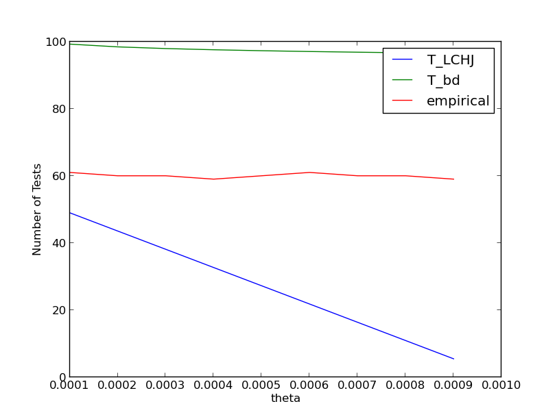
Figure 1: Theoretical lower and upper bounds and empirical Test frequencies as functions of $\theta$

Note that the Upper bound is not optimal and there still is some room for improvement. Note also that the lower bound degrades with $\theta_{i}$. The lower bound ($T_{LCHJ}$) was generated according to Theorem (II.1).

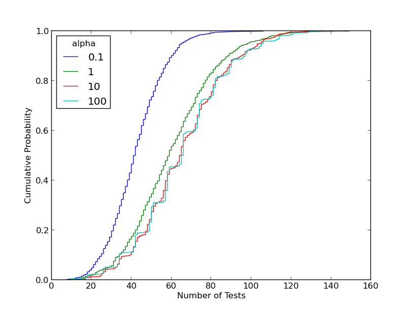
Figure 2: Cumulative success probability distribution curves of the algorithm with fixed $\theta=0.0001$ and varying $\alpha$

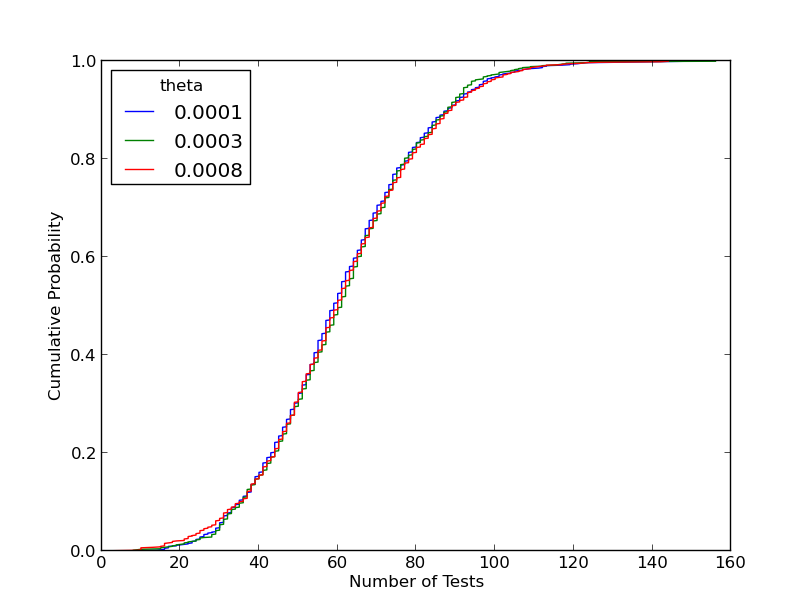
Figure 3: Cumulative success probability distribution curves for fixed $\alpha=1$ and varying $\theta$

Figures (2) and (3) show that the performance is relatively insensitive to the cut-off $\theta$, and more sensitive to the uniformity (or otherwise) of the probability distribution ${\mathbf{p}}$. Heuristically, this is for because distributions which are highly concentrated on a few items algorithms can make substantial savings on the testing budget by testing those highly likely items first (which is captured in the bin structure of the above algorithm).

The insensitivity to the cutoff $\theta$ is due to items below $\theta$ being overwhelmingly unlikely to be defective - which for small $\theta$ means that few items (relative to the size of the problem) get discarded.

V Discussion

We have introduced and analysed an algorithm for Probabilistic group testing which uses ‘just over’ $H({\mathbf{U}})$ tests to recover all the defectives with high probability. Combined with a weak converse taken from [8], this allows us to deduce that the weak capacity of Probabilistic group testing is $C=1$. These results are illustrated by simulation.

For simplicity, this work has concentrated on establishing a bound $T_{{\rm bd}}$ in (17) which has leading term $H({\mathbf{U}})$, and not on tightening bounds on the coefficient of $\mu$ in (17). For completeness, we mention that this coefficient can be reduced from 3, under a simple further condition:

Remark V.1

For some $c\leq 1/2$, we assume that all the $p_{i}\leq c$, and we alter the definition of ‘fullness’ to assume that a set is full if it has total probability less than $\alpha$. In this case, the term $P_{{\mathcal{S}}}\log_{2}P_{{\mathcal{S}}}$ in (9) becomes $P_{{\mathcal{S}}}\log_{2}(\alpha+c)$, the bound in (14) becomes $\mu/\alpha$, and since $\left((1-p)\log_{2}(1-p)\right)/p$ is decreasing in $p$, we can add a term $(1-c)\log_{2}(1-c)$ to (19). Overall, the coefficient of $\mu$ becomes $f(a,c):=\log_{2}(\alpha+c)+1+1/\alpha+(1-c)\log_{2}(1-c)$, which we can optimize over $\alpha$. For example, if $c=1/4$, taking $\alpha=0.88824$, we obtain $f(a,c)=2.00135$.

It remains of interest to tighten the upper bound of Theorem II.1, in order prove a strong converse, and hence confirm that the strong capacity is also equal to $1$.

In future work, we hope to explore more realistic models of defectivity, such as those where the defectivity of $U_{i}$ are not necessarily independent, for example by imposing a Markov neighbourhood structure.

References

- [1] R. Dorfman, “The detection of defective members of large populations,” The Annals of Mathematical Statistics, pp. 436–440, 1943.
- [2] D. Du and F. Hwang, Combinatorial Group Testing and Its Applications, ser. Series on Applied Mathematics. World Scientific, 1993.
- [3] M. Malyutov, “Search for sparse active inputs: a review,” in Information Theory, Combinatorics and Search Theory, ser. Lecture notes in Computer Science. London: Springer, 2013, vol. 7777, pp. 609–647.
- [4] G. Atia and V. Saligrama, “Boolean compressed sensing and noisy group testing,” IEEE Trans. Inform. Theory, vol. 58, no. 3, pp. 1880 –1901, March 2012.
- [5] D. Sejdinovic and O. T. Johnson, “Note on noisy group testing: Asymptotic bounds and belief propagation reconstruction,” in Proceedings of the 48th Annual Allerton Conference on Communication, Control and Computing, 2010, pp. 998–1003.
- [6] M. P. Aldridge, L. Baldassini, and O. T. Johnson, “Group testing algorithms: bounds and simulations,” IEEE Trans. Inform. Theory, vol. 60, no. 6, pp. 3671–3687, 2014.
- [7] T. Wadayama, “An analysis on non-adaptive group testing based on sparse pooling graphs,” in 2013 IEEE International Symposium on Information Theory, 2013, pp. 2681–2685.
- [8] T. Li, C. L. Chan, W. Huang, T. Kaced, and S. Jaggi, “Group testing with prior statistics,” 2014, see arxiv:1401.3667.
- [9] G. Atia, S. Aeron, E. Ermis, and V. Saligrama, “On throughput maximization and interference avoidance in cognitive radios,” in Consumer Communications and Networking Conference, 2008. CCNC 2008. 5th IEEE. IEEE, 2008, pp. 963–967.
- [10] N. Shental, A. Amir, and O. Zuk, “Identification of rare alleles and their carriers using compressed se (que) nsing,” Nucleic acids research, vol. 38, no. 19, pp. e179–e179, 2010.
- [11] L. Baldassini, O. T. Johnson, and M. P. Aldridge, “The capacity of adaptive group testing,” in 2013 IEEE International Symposium on Information Theory, Istanbul Turkey, July 2013, 2013, pp. 2676–2680.
- [12] V. Tan and G. Atia, “Strong impossibility results for sparse signal processing,” IEEE Signal Processing Letters, vol. 21, no. 3, pp. 260–264, March 2014.
- [13] F. K. Hwang, “A method for detecting all defective members in a population by group testing,” Journal of the American Statistical Association, vol. 67, no. 339, pp. 605–608, 1972.
- [14] C. Aksoylar, G. Atia, and V. Saligrama, “Sparse signal processing with linear and non-linear observations: A unified Shannon theoretic approach,” in 2013 IEEE Information Theory Workshop (ITW), Sept 2013, pp. 1–5.
- [15] E. J. Candès, J. Romberg, and T. Tao, “Robust uncertainty principles: Exact signal reconstruction from highly incomplete frequency information,” IEEE Trans. Inform. Theory, vol. 52, no. 2, pp. 489–509, 2006.
- [16] D. L. Donoho, “Compressed sensing,” IEEE Trans. Inform. Theory, vol. 52, no. 4, pp. 1289–1306, 2006.
- [17] V. V. Petrov, Limit Theorems of Probability Theory: Sequences of Independent Random Variables. Oxford: The Clarendon Press, 1995.