Knots, links, anyons and statistical mechanics
of entangled polymer rings

Abstract

The field theory approach to the statistical mechanics of a system of N polymer rings linked together is generalized to the case of links that have a fixed number $2s$ of maxima and minima. Such kind of links are called plats and appear for instance in the DNA of living organisms. The topological states of the link are distinguished using the Gauss linking number. This is a relatively weak link invariant in the case of a general link, but its efficiency improves when $2s-$plats are considered. It is proved that, if we restrict ourselves to $2s-$plat conformations, the field theoretical model established here is able to take into account also the interactions of topological origin involving three chains simultaneously. It is shown that these three-body interactions have nonvanishing contributions when three or more rings are entangled together, enhancing for instance the attractive forces between monomers. The model can be used to study the statistical mechanics of polymers in confined geometries, for instance when $2s$ extrema of a few polymer rings are attached to membranes. Its partition function is mapped here into that of a multi-layer electron gas. Such quasi-particle systems are studied in connection with several interesting applications, including high-$T_{c}$ superconductivity and topological quantum computing. At the end an useful connection with the cosh-Gordon equation is shown.

1 Introduction

Knots and links are a fascinating subject and are researched in connection with several concrete applications both in physics and biology [1, 2, 3, 4, 5, 6, 7, 8, 9, 10, 11, 12, 13, 14, 15, 16, 17, 18, 19, 20, 21, 22, 23, 24, 25, 26]. A beautiful review from a theoretical physics point of view about knot theory and polymers can be found in Ref. [27], Chapter 16. In this paper we study the statistical mechanics of a system of an arbitrary number of entangled polymer rings. Mathematically, two or more entangled polymers form what is called a link. Single polymer rings form instead knots. We will restrict ourselves to systems in the configurations of $2s-$plats. Roughly speaking, $2s-$plats are knots or links obtained by braiding together a set of $2s$ strings and connecting their ends pairwise [28]. A physical realization of $2s-$plats could be that of two rings topologically entangled together and with some of their points attached to two membranes or surfaces. In nature $2s-$plats occur for example in the DNA of living organisms [23, 11, 24, 29]. Indeed, it is believed that most knots and links formed by DNA are in the class of $4-$plats [11]. These biological applications have inspired the research of Ref. [30], in which $4-$plats have been studied with the methods of statistical mechanics and field theory. In particular, in [30] it has been established an analogy between polymeric $4-$plats and anyons, showing in this way the tight relations between two component systems of quasiparticles and the theory of polymer knots and links. After the publication of [30], interesting applications of analogous anyon systems to topological quantum computing have been proposed [31, 32, 33]. These applications are corroborated by the results of experiments concerning the detection of anyons obeying a nonabelian statistics, see for example [34]. While these results have appeared in 2005 and are still under debate [33, 35], other systems in which non-abelian anyon statistics could be present have been discussed [36, 37].

Motivated by these recent advances, we study here the general case of $2s-$plats in which $N$ polymer rings are entangled together to form a link. The topology of the link is distinguished using the Gauss linking number. This is a weak topological invariant, so that many inequivalent topological configurations characterized by some value of the Gauss linking number are allowed. However, since we are restricting ourselves to conformations that, by construction, must remain $2s-$plats, we are implicitly imposing a more stringent topological condition on the system than that imposed merely by the Gauss linking number. For example, both the unlink and the Whitehead link have zero Gauss linking number, but a $4-$plat unlink is not allowed to change into a Whitehead link, which cannot be realized as a $4-$plat. Viceversa, a $6-$plat Whitehead link will not transform into a $4-$plat unlink, despite the fact that both topological configurations share the same value of the Gauss linking number.

Among all knot and link configurations, the class of $2s-$plats is very special. For instance, it is possible to decompose the trajectory of a $2s-$plat into a set of $2s$ open subtrajectories that can be further interpreted as the trajectories of $2s$ polymer chains directed along an arbitrary direction. Without losing generality, we assume that this direction coincides with the $z-$axis. Successively, we map into a field theory the system of $2s-$directed polymers resulting from the decomposition of the plat. After the passage to second quantized fields, a model describing a gas of quasiparticles is obtained. In this model, the $z$ coordinate becomes the "time", while the monomer densities of the $2s$ directed polymers may be interpreted as quasiparticle densities of a multi-layered anyon gas. All the nonlocalities and strong nonlinearities of the original theory due to the topological constraints disappear in the field theoretical formulation. A remarkable feature of polymers in the configuration of a $2s-$plat is that these systems admit self-dual points and their Hamiltonian can be minimized by self-dual solutions of the classical equations of motion. Here we show that in the case of a $4-$plat these solutions may be explicitly constructed after solving a cosh-Gordon equation. The self-dual conformations of a $4-$plat should be particularly stable and, on the other side, with the present technologies [39] it is possible to realize polymer $2s-$plats in the laboratory. Thus there is some hope that some effect related to these conformations could be observable.

Apart from the existence of self-dual solutions, the field theoretical model developed in this work has also phenomenological consequences that are relevant for the statistical mechanics of polymers. First of all, it provides an explicit and nonperturbative expression of the interactions among the monomers arising due to the constraints which fix the topological configuration of the $2s-$plat. After an exact summation over the abelian BF-fields, it turns out that the monomers are subjected to forces of topological origin that have a two-body and a three-body components. The two-body interactions can be both attractive and repulsive, depending on the conformation of the system and strongly interphere with the non-topological interactions, which two-body interactions as well. This results confirms at a nonperturbative level the outcome of a previous calculation performed with the help of the method of the effective potential [53], where it was found that the monomers of two polymer rings attract themselves due to the topological constraints counterfeiting the excluded volume interactions typical of polymers in a good solution. In the particular case of a $4s-$plat, it has been shown in [30] that, after a Bogomol’nyi transformation, it is possible to single out contributions of the two-body forces of topological origin that match exactly, apart from proportionality constants, the excluded volume forces. What is somewhat unespected is the presence of three-body interactions in a polymer system subjected to topological constraints imposed with the help of the Gauss linking number. This is surprising because the Gauss linking number is able to take into account only the topological relations between pairs of trajectories. For this reason, one could expect that this type of constraints is rather associated with interactions between pairs of monomers belonging to two different chains. Indeed, before the second quantization procedure, the explicit expression of the Gauss linking number can be interpreted as a (nonlocal) two-body potential related to forces acting on the bonds located on two different polymers. Three-body forces give a vanishing contribution in the case of links with two polymers only, see Ref. [53]. However, we show here that there are processes in which three-body forces are relevant if the number of loops involved in the link is equal to three or higher.

This paper is organized as follows. Before mapping the partition function of a general $2s-$plat into that of anyons, it is necessary to split the trajectories of the $N$ polymer rings forming the plat into a set of $2s$ subtrajectories. The splitting procedure and the definition of a suitable "time" variable that parametrizes the $2s$ subtrajectories is carefully described in Section 2. In Section 3 it is shown how it is possible to implement and simplify in the partition function of the $2s-$plat the constraints that fix the possible topological configurations in which the system of polymer rings linked together can be found. The constraints are imposed using the Gauss linking number. The treatment follows the method already established in Ref. [41], but its generalization to the case in which the trajectories are splitted into subtrajectories parametrized by the special "time" coordinate instead of the usual arc-lengths is new. To eliminate the nonlinearities and nonlocalities introduced by the topological constraints, which necessarily have memory since they must remember the global geometry of the ring in space, we use a set of abelian BF-fields. Roughly speaking, these fields generate electromagnetic type interactions with the monomers and create in this way the necessary "reaction" forces that forbid the system to escape the constraints. The BF-field theory is quantized in the non-covariant Coulomb gauge, because this leads to several simplifications and is very convenient in order to establish the analogy with anyon systems. How the "covariance" of the theory is recovered is shown in Appendix B in the particular case of a $4-$plat. This example is very helpful to interprete the meaning of the Gauss linking number in the Coulomb gauge, which is apparently more related to the winding number of open trajectories than to the Gauss linking number. In Section 4 the passage from first quantized polymer trajectories to second quantized fields is performed. The case of general interactions between the monomers is considered. After the second quantization procedure and the introduction of replica complex scalar fields, the densities of monomers of the original polymer rings can be regarded as the densities of a system of multilayered gas of quasiparticles. The topological BF-fields are eliminated by integrating them out from the partition function. In Section 5 some phenomenological consequences on the statistical mechanics of the $2s-$plat coming from the field theoretical model obtained in Section 4 are presented. In Section 6 we limit ourselves to $4-$plats, switching off the non-topological interactions. In this particular case, studied in Ref. [30], it is known that the Hamiltonian of the $4-$plat is minimized by self-dual solutions. Here the classical equations of motion are reduced to a cosh-Gordon equation. It is shown how the explicit expression of the classical configurations minimizing the Hamiltonian of the $4-$plat can be constructed out of the solution of this cosh-Gordon equation. Finally, our conclusions are drawn in Section 7.

2 Polymers as $2s-$plats

Let’s consider $N$ closed loops $\Gamma_{1},\ldots,\Gamma_{N}$ of lengths $L_{1},\ldots,L_{N}$ respectively in a three-dimensional space with coordinates $(\boldsymbol{r},z)$. The vector $\boldsymbol{r}=(x,y)$ spans the two dimensional space $\mathbb{R}^{2}$. $z$ will play later on the role of time. The $N$ loops will be labeled using as indices the first letters of the latin alphabet: $a,b,c,\ldots=1,\ldots,N$. We will assume that $\Gamma_{1},\ldots,\Gamma_{N}$ form a $2s-$plat. For convenience, we briefly review what is a $2s-$plat. First of all, we recall that a closed trajectory in the three-dimensional space is from the mathematical point of view a knot, while a system of knots linked together forms a link.

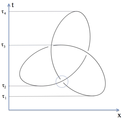
Figure 1: Representation of a trefoil knot in terms as a two-dimensional diagram.

Figure 2: The figure shows one of the crossings which are present in the diagram of the trefoil knot of Fig. 2.

After a projection onto a plane knots and links may be represented by diagrams like those of Fig. 2 and 3, in which the original three-dimensional structure is simulated by a system of crossings, see Fig. 2.

Figure 3: A link formed by two polymers $\Gamma_{1}$ and $\Gamma_{2}$.

Each crossing is composed by three arcs, one overpass and two underpasses. Giving an orientation to the trajectories, we can distinguish positive and negative crossings, see Fig. 4.

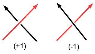
Figure 4: Left and right crossings of the elements of two oriented paths.

One may also realize that the trefoil diagram in Fig. 2 is characterized by two minima and two maxima. Two dimensional diagrams of this kind, deformed in such a way that the number $2s$ of minima and maxima is the smallest possible and the maxima and minima are aligned at the same heights $z_{\max}$ and $z_{\min}$ respectively, are called in knot theory $2s-$plats . The height of a $2s-$plat is measured here with respect to the $z$ axis. In the present case, with some abuse of language, we will call $2s-$plats any system of $N$ three-dimensional knots realized in such a way that the trajectories of the knots are characterized by a number $2s$ of maxima and minima. The locations of the $s$ points of maxima and those of the $s$ points of minima are fixed, i. e. they are not allowed to fluctuate and their number $2s$ is constant. The points of maxima and minima do not need to be aligned as it happens in the mathematical definition of a $2s-$plat. An example of the two-dimensional diagram of such a physical $2s-$plat is given in Fig. 3. Let us denote with the symbols $\tau_{a,I_{a}}$, $I_{a}=0,\ldots,2s_{a}-1$, the heights of the maxima and minima of each trajectory $\Gamma_{a}$, for $a=1,\ldots,N$. Of course, it should be that

$$\sum_{a=1}^{N}s_{a}=s.$$ (1)

We choose $\tau_{a,0}$ to be the height of the absolute minimum of each trajectory $\Gamma_{a}$. Starting from $\tau_{a,0}$, we select the orientation of $\Gamma_{a}$ in such a way that, proceeding along the trajectory according to that orientation, we will encounter in the order the points $\tau_{a,1},\tau_{a,2},\ldots,\tau_{a,2s_{a}}$. Clearly, $\tau_{a,1}$ is the height of a point of maximum, $\tau_{a,2}$ the height of a minimum and so on. Moreover, we should put for consistency

$$\tau_{a,2s_{a}}\equiv\tau_{a,0}.$$ (2)

The introduction of two symbols for the same height $\tau_{a,0}$ will be useful in the future in order to write formulas in a more compact form. In the following, the trajectories $\Gamma_{1},\ldots,\Gamma_{N}$ will be decomposed into a set of directed trajectories $\Gamma_{a,I_{a}}$, $a=1,\ldots,N$ and $I_{a}=1,\ldots,2s_{a}$, whose ends are made to coincide in such a way that they form the topological configuration of two linked rings. An example when $s=3$ and $N=1$ is presented in Fig. 5.

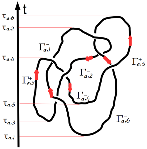
Figure 5: Sectioning procedure for a $2s$-plat $\Gamma_{a}$ with $s=3$.

In the general case, the set of points belonging to $\Gamma_{a,I_{a}}$ can be described by the formula:

$$\Gamma_{a,I_{a}}=\left\{\boldsymbol{r}_{a,I_{a}}(z_{a,I_{a}})\left|\begin{array}[]{c}a=1,\ldots,N;\qquad I_{a}=1,\ldots,2s_{a}\\ \left\{\begin{array}[]{rcl}\tau_{a,I_{a}-1}\leq z_{a,I_{a}}\leq\tau_{a,I_{a}}\qquad I_{a}\mbox{ odd}\\ \tau_{a,I_{a}}\leq z_{a,I_{a}}\leq\tau_{a,I_{a}-1}\qquad I_{a}\mbox{ even}\end{array}\right.\end{array}\right.\right\}$$ (3)

where the additional conditions:

$$\boldsymbol{r}_{a,I_{a}}(\tau_{a,I_{a}}) = \boldsymbol{r}_{a,I_{a}+1}(\tau_{a,I_{a}})\qquad I_{a}=1,\ldots,2s_{a}-1$$ (4)

$$\boldsymbol{r}_{a,1}(\tau_{a,0}) = \boldsymbol{r}_{a,2s_{a}}(\tau_{a,0})$$ (5)

are understood. These conditions are needed in order to connect together the subtrajectories $\Gamma_{a,I_{a}}$ so that the loop $\Gamma_{a}$ is reconstructed. In Eq. (3) the two-dimensional vector $\boldsymbol{r}_{a,I_{a}}(z_{a,I_{a}})$ represents the projection of the trajectory $\Gamma_{a,I_{a}}$ onto the plane $x,y$ perpendicular to the $z-$axis. Let us note that we are using the same indexes $I_{a}$ to label the trajectories $\Gamma_{a,I_{a}}$ and the points $\tau_{a,I_{a}}$. However, in the first case $I_{a}=1,\ldots,2s_{a}$, while in the second case we have chosen $I_{a}=0,\ldots,2s_{a}-1$. The range of the indices $I_{a}$ in the variables $z_{a,I_{a}}$’s and of the $t_{a,I_{a}}$’s that will be defined later is the same as that of the indices labeling the trajectories $\Gamma_{a,I_{a}}$’s, i. e. $I_{a}=1,\ldots,2s_{a}$.

We notice that the $z_{a,I_{a}}$’s are always growing. In this way, the fact that the whole chain is continuous and has a given orientation is not taken into account. Better variables, respecting both the continuity and orientation of the trajectories $\Gamma_{a,I_{a}}$, are the $t_{a,I_{a}}$’s, which are defined as follows:

$$t_{a,I_{a}}=z_{a,I_{a}} \mbox{when }I_{a}\mbox{ is odd}$$ (6)

$$t_{a,I_{a}}=-(z_{a,I_{a}}-\tau_{a,I_{a}})+\tau_{a,I_{a}-1} \mbox{when }I_{a}\mbox{ is even}.$$ (7)

Assuming for instance that $I_{a}$ is odd, then for any two consecutive trajectories $\Gamma_{a,I_{a}}$ and $\Gamma_{a,I_{a+1}}$ the range of the variables $t_{a,I_{a}}$ and $t_{a,I_{a+1}}$ is given by:

$$\tau_{a,I_{a}-1}\leq t_{a,I_{a}}\leq\tau_{a,I_{a}}\qquad I_{a}\mbox{ odd}\qquad 1\leq I_{a}\leq 2s_{a}-1$$ (8)

Instead, if $I_{a}$ is even:

$$\tau_{a,I_{a}-1}\geq t_{a,I_{a}}\geq\tau_{a,I_{a}}\qquad I_{a}\mbox{ even}\qquad 2\leq I_{a}\leq 2s_{a}.$$ (9)

Let us recall that by our conventions the trajectories labeled by odd $I_{a}$’s are oriented from a point of minimum to a point of maximum, while trajectories with even values of $I_{a}$ go from a point of maximum to a point of minimum. Accordingly, the new variables $t_{a,I_{a}}$ have been chosen in such a way that they increase from the minimum to the maximum when $I_{a}$ is odd, while they decrease from the point of maximum to that of minimum when $I_{a}$ is even. Finally, we provide the definition of the curves $\Gamma_{a,I_{a}}$ parametrized with the help of the $t_{a,I_{a}}$’s:

$$\Gamma_{a,I_{a}}=\left\{\boldsymbol{r}_{a,I_{a}}(t_{a,I_{a}})\left|\begin{array}[]{c}a=1,\ldots,N;\qquad I_{a}=1,\ldots,2s_{a}\\ \left\{\begin{array}[]{rcl}\tau_{a,I_{a}-1}\leq t_{a,I_{a}}\leq\tau_{a,I_{a}}\qquad I_{a}\mbox{ odd}\\ \tau_{a,I_{a}-1}\geq t_{a,I_{a}}\geq\tau_{a,I_{a}}\qquad I_{a}\mbox{ even}\end{array}\right.\end{array}\right.\right\}$$ (10)

Of course, the boundary conditions (4) and (5) are always understood.

The variables $t_{a,I_{a}}$ arise in a natural way when a curvilinear integral around the loop $\Gamma_{a}$ is split into many subtrajectories $\Gamma_{a,I_{a}}$. In fact, let’s consider for example integrals of the kind

$$I=\oint_{\Gamma_{a}}d{\tilde{x}}^{\mu}_{a}(d_{a})A_{\mu}({\tilde{x}}_{a}(d_{a}))$$ (11)

where the symbol ${\tilde{x}}^{\mu}_{a}(d_{a})=({\tilde{\boldsymbol{r}}_{a}}(d_{a}),{\tilde{x}}_{a}^{3}(d_{a}))$ denotes the points of the trajectory $\Gamma_{a}$ parametrized in terms of the arc-length $d_{a}$, $0\leq d_{a}\leq L_{a}$. $A_{\mu}({\tilde{x}}_{a}(d_{a}))$ is an abelian gauge field on ${\mathbb{R}}^{3}$. It is easy to show that, after splitting the loop $\Gamma_{a}$ into the subtrajectories $\Gamma_{a,I_{a}}$, on each of these subtrajectories it is possible to change the arc-length $d_{a}$ with the parameters $t_{a,I_{a}}$. If one does that, the curvilinear integral $I$ of Eq. (11) becomes parametrized by the variables $t_{a,I_{a}}$ and may be expressed as follows

$$I=\sum_{I_{a}=1}^{2s_{a}}\int_{\tau_{a,I_{a}-1}}^{\tau_{a,I_{a}}}\left[\frac{d\boldsymbol{r}_{a,I_{a}}(t_{a,I_{a}})}{dt_{a,I_{a}}}\cdot\boldsymbol{A}(\boldsymbol{r}_{a,I_{a}}(t_{a,I_{a}}),t_{a,I_{a}})+A_{3}(\boldsymbol{r}_{a,I_{a}}(t_{a,I_{a}}),t_{a,I_{a}})\right]$$ (12)

where

$$t_{a,I_{a}}={\tilde{x}}^{3}_{a}(d_{a})\qquad\qquad\boldsymbol{r}_{a,I_{a}}(t_{a,I_{a}})=\boldsymbol{r}_{a,I_{a}}({\tilde{x}}_{a}^{3}(d_{a}))={\tilde{\boldsymbol{r}}_{a}}(d_{a}).$$ (13)

Of course, the above equation is valid only if $d_{a}$ is restricted on the trajectory $\Gamma_{a,I_{a}}$, i.e., $\delta_{a,I_{a}-1}\leq d_{a}\leq\delta_{a,I_{a}}$. The $\delta_{a,I_{a}}$’s denote the values of the arc-length at the points of maxima and minima of the $2s_{a}-$plat $\Gamma_{a}$. Clearly, ${\tilde{x}}_{a}^{3}(\delta_{a,I_{a}})=\tau_{a,I_{a}}$.

3 Fixing the topological properties of a $2s-$plat: the case of the Gauss linking number

In the case of a $2s-$plat composed by $N$ loops $\Gamma_{1},\ldots,\Gamma_{N}$, it is possible to specify the winding number between any two subtrajectories $\Gamma_{a,I_{a}}$ and $\Gamma_{b,I_{b}}$ composing the plat. These winding numbers cannot change due to the thermal fluctuations, because the end points $(\boldsymbol{r}(\tau_{a,I_{a}-1}),\tau_{a,I_{a}-1})$ and $(\boldsymbol{r}(\tau_{a,I_{a}}),\tau_{a,I_{a}})$ of each subtrajectory $\Gamma_{a,I_{a}}$ must be fixed in our construction. This fact can be used to constrain the $2s-$plat to stay in very complex topological configurations. In the following, however, we will not adopt this strategy. The topological configurations of the system will rather be imposed as in Refs. [41] by applying the Gauss linking number.

3.1 The standard approach of imposing the constraints with the Gauss linking number

The Gauss linking number is a link invariant expressing the topological states of two closed trajectories linked together. Due to the fact that it can only be applied to pairs of loops, here we restrict ourselves for simplicity to the case of a $2s-$plat composed by only two loops $\Gamma_{1}$ and $\Gamma_{2}$. Note that each of these two loops is a plat too having $s_{a}$ points of maxima and $s_{a}$ points of minima with $a=1,2$. For consistency, it should be that $s=s_{1}+s_{2}$. The Gaussian linking number is defined as follows

$$\chi(\Gamma_{1},\Gamma_{2})=\frac{1}{4\pi}\epsilon_{\mu\nu\rho}\oint_{\Gamma_{1}}d\tilde{x}^{\mu}_{1}(d_{1})\oint_{\Gamma_{2}}d\tilde{x}^{\nu}_{2}(d_{2})\frac{(\tilde{x}_{1}(d_{1})-\tilde{x}_{2}(d_{2}))^{\rho}}{|\tilde{x}_{1}(d_{1})-\tilde{x}_{2}(d_{2})|^{3}}$$ (14)

where the $\tilde{x}^{\mu}_{a}(d_{a})$’s and the arc-lengths $d_{a}$’s, $a=1,2$ have been already defined at the end of the previous Section, after Eq. (11). The trajectories of the two loops will be topologically constrained by the condition

$$m_{12}=\chi(\Gamma_{1},\Gamma_{2})$$ (15)

$m_{12}$ being a given integer. The above constraint is imposed by inserting the Dirac delta function $\delta(m_{12}-\chi(\Gamma_{1},\Gamma_{2}))$ in the partition function of the $2s-$plat, where the statistical sum over all conformations of $\Gamma_{1}$ and $\Gamma_{2}$ is performed. Of course, the analytical treatment of such a delta function in a path integral is difficult. Some simplification is obtained by passing to the Fourier representation

$$\delta(m_{12}-\chi(\Gamma_{1},\Gamma_{2}))=\int_{-\infty}^{+\infty}\frac{d\lambda_{12}}{\sqrt{2\pi}}\;{\rm e}^{-i\lambda_{12}(m_{12}-\chi(\Gamma_{1},\Gamma_{2}))}.$$ (16)

Even in the Fourier representation, the difficulty of having to deal with the Gauss linking number in the exponent appearing in the right hand side of Eq. (16) remains. Formally, this link invariant introduces a term that resembles the potential of a two-body interaction which is both nonlocal and nonpolynomial. For this reason, the treatment of the Gauss linking number in any microscopical model of topologically entangled polymers is complicated. The best strategy to deal with this problem consists in rewriting the delta function $\delta(m_{12}-\chi(\Gamma_{1},\Gamma_{2}))$ as a correlation function of the holonomies of a local field theory, namely the so-called abelian BF-model [41, 42, 48]

$$\delta(m_{12}-\chi(\Gamma_{1},\Gamma_{2}))=\int_{-\infty}^{+\infty}d\lambda_{12}\;{\rm e}^{-i\lambda_{12}m_{12}}{{\cal Z}}_{\rm BF}(\lambda_{12})$$ (17)

where

$${{\cal Z}_{\rm BF}}(\lambda_{12}) = \int{\cal D}B_{\mu}^{12}(x){\cal D}C_{\mu}^{12}(x)\;{\rm e}^{-iS_{\rm BF}\left[B,C\right]}$$ (18)

$$\times \;{\rm e}^{-i\tilde{c}_{12}\oint_{\Gamma_{1}}d\tilde{x}^{\mu}_{1}(d_{1})B_{\mu}^{12}(\tilde{x}_{1}(d_{1}))}\;{\rm e}^{-i\tilde{d}\oint_{\Gamma_{2}}d\tilde{x}^{\mu}_{2}(d_{2})C_{\mu}^{12}(\tilde{x}_{2}(d_{2}))}.$$

In the above equation we have put $x\equiv(\boldsymbol{x},t)$ to be dummy integration variables spanning the whole three-dimensional space $\mathbb{R}^{3}$. Moreover, $S_{\rm BF}[B,C]$ denotes the action of the abelian BF-model

$$S_{\rm BF}[B,C]=\frac{\kappa}{4\pi}\int d^{3}xB_{\mu}^{12}(x)\partial_{\nu}C_{\rho}^{12}(x)\epsilon^{\mu\nu\rho}.$$ (19)

Above $\epsilon^{\mu\nu\rho}$, $\mu,\nu,\rho=1,2,3$, is the completely antisymmetric $\epsilon-$tensor density defined by the condition $\epsilon^{123}=1$. $\kappa$ is the coupling constant of the BF-model. Finally, the constants $\tilde{c}_{12}$ and $\tilde{d}$ are given by:

$$\tilde{c}_{12}=\lambda_{12}\qquad\qquad\tilde{d}=\frac{\kappa}{8\pi^{2}}.$$ (20)

While there is some freedom in choosing $\tilde{c}_{12}$ and $\tilde{d}$, one unavoidable requirement in order that Eq. (17) will be satisfied is that one of these parameters should be linearly dependent on $\kappa$. In this way, it is easy to check that $\kappa$ may be completely eliminated from Eq. (18) by performing a rescaling of one of the two fields $B_{\mu}^{12}$ and $C_{\mu}^{12}$. This is an expected result, because $\kappa$ does not appear in the left hand side of Eq. (17), so that it cannot be a new parameter of the theory. By introducing the currents:

$$\zeta_{12}^{\mu}(x)=\tilde{c}_{12}\oint_{\Gamma_{1}}d\tilde{x}_{1}^{\mu}(d_{1})\delta^{(3)}(x-\tilde{x}_{1}(d_{1}))\qquad\qquad\xi_{12}^{\mu}(x)=\tilde{d}\oint_{\Gamma_{2}}d\tilde{x}_{2}^{\mu}(d_{2})\delta^{(3)}(x-\tilde{x}_{2}(d_{2}))$$ (21)

${\cal Z}_{\rm BF}(\lambda_{12})$ may be rewritten in the more compact way:

$${\cal Z}_{\rm BF}(\lambda_{12}) = \int{\cal D}B_{\mu}^{12}(x){\cal D}C_{\mu}^{12}(x)\;{\rm e}^{-iS_{\rm BF}[B,C]}\;{\rm e}^{-i\int d^{3}x\left[\zeta^{\mu}_{12}(x)B_{\mu}^{12}(x)+\xi_{12}^{\mu}(x)C_{\mu}^{12}(x)\right]}.$$ (22)

With Eq. (22) the goal of transforming the nonlinear and nonlocal interaction appearing in the right hand side of Eq. (16) is achieved. The right hand side of Eq. (22) represents in fact a local field theory, the BF-model, interacting with the trajectories $\Gamma_{1}$ and $\Gamma_{2}$. Of course, the price paid for that simplification is the introduction of the fields $B_{\mu}^{12}$ and $C_{\mu}^{12}$.

3.2 How to impose constraints on a link composed by plats using the Gauss linking number

In all the above discussion, the two trajectories $\Gamma_{1}$ and $\Gamma_{2}$ have been parametrized with the help of the arc-lengths $d_{1}$ and $d_{2}$. However, in the present case the loops $\Gamma_{1},\ldots,\Gamma_{N}$ are realized as a set of open paths $\Gamma_{a,I_{a}}$ connected together by the conditions (4)–(5). The subtrajectories $\Gamma_{a,I_{a}}$’s are directed paths $\boldsymbol{r}_{a,I_{a}}(t_{a,I_{a}})=(x^{1}_{a,I_{a}}(t_{a,I_{a}}),x^{2}_{a,I_{a}}(t_{a,I_{a}}))$ parametrized by the variables $t_{a,I_{a}}$. This difference of parametrization introduces several important changes. Apart from the fact that we have to deal with many subtrajectories, also one degree of freedom, represented by the third coordinate $x^{3}_{a}(s_{a})$, disappears due to the change (13). As a consequence, the method illustrated in the previous Subsection in order to express the Gauss linking number as an amplitude of the BF-model, in particular Eq. (17), should be changed appropriately. Thus, we rewrite the partition function ${\cal Z}_{\rm BF}(\lambda_{12})$ of Eq. (18) using the variables $t_{a,I_{a}}$ to parametrize the subtrajectories $\Gamma_{a,I_{a}}$. The way in which the curvilinear integrals along the loops $\Gamma_{1}$ and $\Gamma_{2}$ appearing in Eq. (18) should be replaced by integrals over the subtrajectories $\Gamma_{a,I_{a}}$ is shown in Eqs. (11) and (12). As a result, we arrive at the following expression of the partition function ${\cal Z}_{\rm BF}(\lambda_{12})$:

$${\cal Z}_{\rm BF}(\lambda_{12}) = \int{\cal D}B_{\mu}^{12}(x){\cal D}C_{\mu}^{12}(x)\;{\rm e}^{-S_{\rm BF}[B,C]}\;{\rm e}^{-i\int d^{3}x\left[\boldsymbol{\zeta}_{12}(\boldsymbol{x},t)\cdot\boldsymbol{B}^{12}(\boldsymbol{x},t)+\zeta^{3}_{12}(\boldsymbol{x},t)B_{3}^{12}(\boldsymbol{x},t)\right]}$$ (23)

$$\times \;{\rm e}^{-i\int d^{3}x\left[\boldsymbol{\xi}_{12}(\boldsymbol{x},t)\cdot\boldsymbol{C}^{12}(\boldsymbol{x},t)+\xi^{3}_{12}(\boldsymbol{x},t)C_{3}^{12}(\boldsymbol{x},t)\right]}$$

where $S_{\rm BF}[B,C]$ coincides with the action (19) and

$$\boldsymbol{\zeta}_{12}(\boldsymbol{x},t) = \tilde{c}_{12}\sum_{I_{1}=1}^{2s_{1}}\int_{\tau_{1,I_{1}-1}}^{\tau_{1,I_{1}}}dt_{1,I_{1}}\dot{\boldsymbol{r}}_{1,I_{1}}(t_{1,I_{1}})\delta^{(2)}(\boldsymbol{x}-\boldsymbol{r}_{1,I_{1}}(t_{1,I_{1}}))\delta(t-t_{1,I_{1}})$$ (24)

$$\boldsymbol{\xi}_{12}(\boldsymbol{x},t) = \tilde{d}\sum_{I_{2}=1}^{2s_{2}}\int_{\tau_{2,I_{2}-1}}^{\tau_{2,I_{2}}}dt_{2,I_{2}}\dot{\boldsymbol{r}}_{2,I_{2}}(t_{2,I_{2}})\delta^{(2)}(\boldsymbol{x}-\boldsymbol{r}_{2,I_{2}}(t_{2,I_{2}}))\delta(t-t_{2,I_{2}})$$ (25)

$$\zeta_{12}^{3}(\boldsymbol{x},t) = \tilde{c}_{12}\sum_{I_{1}=1}^{2s_{1}}\int_{\tau_{1,I_{1}-1}}^{\tau_{1,I_{1}}}dt_{1,I_{1}}\delta^{(2)}(\boldsymbol{x}-\boldsymbol{r}_{1,I_{1}}(t_{1,I_{1}}))\delta(t-t_{1,I_{1}})$$ (26)

$$\xi_{12}^{3}(\boldsymbol{x},t) = \tilde{d}\sum_{I_{2}=1}^{2s_{2}}\int_{\tau_{2,I_{2}-1}}^{\tau_{2,I_{2}}}dt_{2,I_{2}}\delta^{(2)}(\boldsymbol{x}-\boldsymbol{r}_{2,I_{2}}(t_{2,I_{2}}))\delta(t-t_{2,I_{2}}).$$ (27)

3.3 The Coulomb gauge

Now we use the Fourier representation of the topological constraints of Eq. (17), but with the partition function ${\cal Z}_{\rm BF}(\lambda_{12})$ written in the form of Eq. (23). In this way the path integral over all conformations of the $2s-$plat can be split into path integrals over all conforations of the subtrajectories $\Gamma_{a,I_{a}}$. The latter can be regarded as the trajectories of a two-dimensional system of $2s$ particles interacting with abelian BF fields. In order to establish an explicit analogy between polymers and two-dimensional particles evolving in time, it is convenient to choose a non-covariant gauge like the Coulomb gauge. Similar approaches like that proposed here can be found in [49, 50]. Interestingly, in [50] Chern-Simons field theories quantized in noncovariant gauges have also been applied to express the knot and link invariants of $2s-$plats, called in [50] Morse knots. In Refs. [49] and [50] knots and links are however static, they do not fluctuate, and the calculations have been performed in noncovariant gauges different from the Coulomb gauge.

To begin with, we impose the Coulomb gauge condition on the $B$ and $C$ fields

$$\partial^{i}B_{i}^{12}=\partial^{i}C^{12}_{i}=0$$ (28)

where $i=1,2$ labels the first two components of the vector potentials $B_{\mu}^{12}=(\boldsymbol{B}^{12},B_{3}^{12})$ and $C_{\mu}^{12}=(\boldsymbol{C}^{12},C_{3}^{12})$. After the gauge choice (28), the action of the BF model (19) becomes

$$S_{\rm BF,CG}\left[B,C\right]=\frac{\kappa}{4\pi}\int\!d^{3}x\left[B^{12}_{3}\epsilon^{ij}\partial_{i}C^{12}_{j}+C_{3}^{12}\epsilon^{ij}\partial_{i}B_{j}^{12}\right]$$ (29)

with $\epsilon^{ij}=\epsilon^{ij3}$ being the two-dimensional completely antisymmetric tensor. The gauge fixing term vanishes in the pure Coulomb gauge where the conditions (28) are strictly satisfied. Also the Faddeev-Popov term, which in principle should be present in Eq. (29), may be neglected because the ghosts decouple from all other fields.

The requirement of transversality of (28) in the "spatial" directions $x^{1},x^{2}$ implies that the components $B_{i}^{12}$ and $C_{i}^{12}$ of the BF fields may be expressed in terms of two scalar fields $b^{12}$ and $c^{12}$ via the Hodge decomposition:

$$B_{i}^{12}=\epsilon_{ij}\partial^{j}b^{12}\qquad\qquad C_{i}^{12}=\epsilon_{ij}\partial^{j}c^{12}.$$ (30)

After performing the above substitutions of fields in the BF action of Eq. (29), we obtain

$$S_{\rm BF,CG}[B,C]=\frac{\kappa}{4\pi}\int d^{3}x[B_{3}^{12}\Delta c^{12}+C_{3}^{12}\Delta b^{12}].$$ (31)

Now we compute the propagator of the BF fields

$$G_{\mu\nu}(\boldsymbol{x},t;\boldsymbol{y},t^{\prime})=\langle B_{\mu}^{12}(\boldsymbol{x},t),C_{\nu}^{12}(\boldsymbol{y},t^{\prime})\rangle.$$ (32)

Only the following components of the propagator are different from zero:

$$G_{3i}(\boldsymbol{x},t;\boldsymbol{y},t^{\prime})=\frac{\delta(t-t^{\prime})}{2\kappa}\epsilon_{ij}\partial_{\boldsymbol{y}}^{j}\log|\boldsymbol{x}-\boldsymbol{y}|^{2}$$ (33)

$$G_{i3}(\boldsymbol{x},t;\boldsymbol{y},t^{\prime})=-G_{3i}(\boldsymbol{x},t;\boldsymbol{y},t^{\prime}).$$ (34)

The path integration over the scalar fields $b^{12}$ and $c^{12}$ in the partition function ${\cal Z}_{\rm BF}(\lambda)$ is gaussian and can be performed analytically eliminating completely the gauge fields. A natural question that arise at this point is the interpretation of the topological constraint (15) in the Coulomb gauge. As a matter of fact, the BF propagator in the Coulomb gauge breaks explicitly the invariance of the BF model under general three-dimensional transformation. It seems thus hard to recover the form (14) of the Gauss linking number in this gauge. Of course, an equivalent constraint should be obtained in the Coulomb gauge due to gauge invariance. In Appendix B it will be shown by a direct calculation in the case of a $4-$plat that this is actually true. The computation of the expression of the equivalent of the Gauss linking number in the Coulomb gauge for a general $2s$-plat is however technically complicated and will not be performed here.

4 The partition function of a plat

4.1 Directed polymers with topological constraints

In order to write the partition function of a $2s-$plat, we follow the strategy explained in the previous Section of dividing each trajectory $\Gamma_{a}$, $a=1,\ldots,N$, into $2s_{a}$ open paths $\Gamma_{a,I_{a}}$, $I_{a}=1,\ldots,2s_{a}$. The statistical sum ${\cal Z}_{\rm pol}(\{m\})$ of the system is performed over all conformations $\boldsymbol{r}_{a,I_{a}}(t_{a,I_{a}})$ of the subtrajectories $\Gamma_{a,I_{a}}$ using path integral methods, i.e.:

$${\cal Z}_{\rm pol}(\{m\})=\int\limits_{\mbox{\scriptsize boundary}\atop{\mbox{\scriptsize conditions}}}\!\left[\prod_{a=1}^{N}\prod_{I_{a}=1}^{2s_{a}}{\cal D}\boldsymbol{r}_{a,I_{a}}(t_{a,I_{a}})\right]\,{\rm e}^{-(S_{\rm free}+S_{\rm EV})}\prod_{a=1}^{N-1}\prod_{b=a+1}^{N}\delta\left(m_{ab}-\chi(\Gamma_{a},\Gamma_{b})\right).$$ (35)

In the above equation the boundary conditions on the trajectories $\boldsymbol{r}_{a,I_{a}}(t_{a,I_{a}})$ enforce the constraints (4) and (5). The free part of the action $S_{\rm free}$ is given by

$$S_{\rm free}=\sum_{a=1}^{N}\sum_{I_{a}=1}^{2s_{a}}\int_{\tau_{a,I_{a}-1}}^{\tau_{a,I_{a}}}\!dt_{a,I_{a}}(-1)^{I_{a}-1}g_{a,I_{a}}\left|\frac{d\boldsymbol{r}_{a,I_{a}}(t_{a,I_{a}})}{dt_{a,I_{a}}}\right|^{2}.$$ (36)

The parameters $g_{a,I_{a}}>0$ are proportional to the inverse of the Kuhn lengths of the trajectories $\Gamma_{a,I_{a}}$. They are also related to the total lengths of the trajectories $\Gamma_{a,I_{a}}$ according to the formula provided in Appendix A. Let us note that $S_{\rm free}$ is a positive definite functional thanks to the factors $(-1)^{I_{a}-1}$, which compensate the fact that the increment $dt_{a,I_{a}}$ is negative when $I_{a}$ is even. The contribution $S_{\rm EV}$ to the total action takes into account the interactions between the monomers which arise because we treat the subtrajectories $\Gamma_{a,I_{a}}$ as directed paths moving in a random media. The mechanism through which these interactions appear after the integration over the non-white random noises is explained in Ref. [44]. Explicitly, $S_{\rm EV}$ is given by

$$S_{\rm EV} = \frac{1}{2}\sum_{a=1}^{N}\sum_{b=1}^{N}\sum_{I_{a}=1}^{2s_{a}}\sum_{I_{b}=1}^{2s_{b}}\int_{\tau_{a,I_{a}-1}}^{\tau_{a,I_{a}}}dt_{a,I_{a}}\int_{\tau_{b,I_{b}-1}}^{\tau_{b,I_{b}}}dt_{b,I_{b}}(-1)^{I_{a}+I_{b}-2}{\cal M}^{a,I_{a};b,I_{b}}$$ (37)

$$V\left(\boldsymbol{r}_{a,I_{a}}(t_{a,I_{a}})-\boldsymbol{r}_{b,I_{b}}(t_{b,I_{b}})\right)\delta\left(t_{a,I_{a}}-t_{b,I_{b}}\right)$$

where

$${\cal M}^{a,I_{a};b,I_{b}}=\left\{\begin{array}[]{l}0\qquad\mbox{if $a=b$ and $I_{a}=I_{b}$}\\ 1\qquad\mbox{otherwise}\end{array}\right.$$ (40)

Due to the matrix ${\cal M}^{a,I_{a};b,I_{b}}$ the interactions between a subtrajectory with itself are forbidden. We note that the presence of the delta functions $\delta\left(t_{a,I_{a}}-t_{b,I_{b}}\right)$ is necessary to express the fact that the trajectories $\Gamma_{a,I_{a}}$ and $\Gamma_{b,I_{b}}$ for $I_{a}\neq I_{b}$ may interact only if both $t_{a,I_{a}}$ and $t_{b,I_{b}}$ belong to the common interval $[\tau_{a,I_{a}-1},\tau_{a,I_{a}}]\cap[\tau_{b,I_{b}-1},\tau_{b,I_{b}}]$. The potential $V(\boldsymbol{r})$ can be any two-body potential. If the random noises are gaussianly distributed as in Ref. [44], then

$$V(\boldsymbol{r})=V_{0}\delta(\boldsymbol{r})$$ (41)

$V_{0}$ being a positive constant. Again, the factors $(-1)^{I_{a}+I_{b}-2}$ appearing in $S_{\rm EV}$ are necessary in order to compensate the fact that the increments $dt_{a,I_{a}}$ and $dt_{b,I_{b}}$ are negative for even values of $I_{a}$ and $I_{b}$ respectively. Finally, the Dirac delta functions inserted in the right hand side of Eq. (35) impose the topological constraints on each pair of trajectories $(\Gamma_{a},\Gamma_{b})$, $a=1,\ldots,N-1$, $b=a+1,\ldots,N$.

4.2 Passage to Field Theory I: the topological states

According to Eq. (17), the physically relevant contributions coming from the topological conditions $m_{ab}=\chi(\Gamma_{a},\Gamma_{b})$ , $a=1,\ldots,N-1$, $b=a+1,\ldots,N$, are encoded in the Fourier transform ${\cal Z}_{\rm pol}(\{\lambda\})$ of the original probability function ${\cal Z}_{\rm pol}(\{m\})$. Notice that ${\cal Z}_{\rm pol}(\{\lambda\})$ is obtained from ${\cal Z}_{\rm pol}(\{m\})$ by the relation

$${\cal Z}_{\rm pol}(\{m\})=\prod_{a=1}^{N-1}\prod_{b=a+1}^{N}\int_{-\infty}^{+\infty}d\lambda_{ab}\,{\rm e}^{-i\lambda_{ab}m_{ab}}\,{\cal Z}_{\rm pol}(\{\lambda\}).$$ (42)

It is easy to realize that

$${\cal Z}_{\rm pol}(\{\lambda\}) = \int\!\left[\prod_{a=1}^{N-1}\prod_{b=a+1}^{N}{\cal D}B_{\mu}^{ab}{\cal D}C_{\mu}^{ab}\right]{\rm e}^{-iS_{\rm BF}}$$ (43)

$$\int\limits_{\mbox{\scriptsize boundary}\atop{\mbox{\scriptsize conditions}}}\left[\prod_{a=1}^{N}\prod_{I_{a}=1}^{2s_{a}}\!{\cal D}\boldsymbol{r}_{a,I_{a}}(t_{a,I_{a}})\right]{\rm e}^{-(S_{\rm free}+S_{\rm EV}+S_{\rm top})}$$

where

$$S_{\rm BF}=\sum_{a=1}^{N-1}\sum_{b=a+1}^{N}\frac{\kappa}{4\pi}\int\!d^{3}xB_{\mu}^{ab}(x)\partial_{\nu}C_{\rho}^{ab}(x)\epsilon^{\mu\nu\rho}$$ (44)

and

$$S_{\rm top}=i\sum_{a=1}^{N-1}\sum_{b=a+1}^{N}\lambda_{ab}\sum_{I_{a}=1}^{2s_{a}}\int_{\tau_{a,I_{a}-1}}^{\tau_{a,I_{a}}}dt_{a,I_{a}} \left[\dot{\boldsymbol{r}}_{a,I_{a}}(t_{a,I_{a}})\cdot\boldsymbol{B}^{ab}\left(\boldsymbol{r}_{a,I_{a}}(t_{a,I_{a}}),t_{a,I_{a}}\right)\right.$$

$$\left.+B^{ab}_{3}\left(\boldsymbol{r}_{a,I_{a}}(t_{a,I_{a}}),t_{a,I_{a}}\right)\right]$$

$$+\frac{i\kappa}{8\pi^{2}}\sum_{a=1}^{N-1}\sum_{b=a+1}^{N}\sum_{I_{b}=1}^{2s_{b}}\int_{\tau_{b,I_{b}-1}}^{\tau_{b,I_{b}}}dt_{b,I_{b}} \left[\dot{\boldsymbol{r}}_{b,I_{b}}(t_{b,I_{b}})\cdot\boldsymbol{C}^{ab}\left(\boldsymbol{r}_{b,I_{b}}(t_{b,I_{b}}),t_{b,I_{b}}\right)\right.$$ (45)

$$\left.+C^{ab}_{3}\left(\boldsymbol{r}_{b,I_{b}}(t_{b,I_{b}}),t_{b,I_{b}}\right)\right].$$

After going back to the parametrization of the loops $\Gamma_{a}$ with the help of the arc-lengths using Eqs. (11) and (12) and integrating out the BF fields, it is possible to recover in the expression of ${\cal Z}_{\rm pol}(\{\lambda\})$ the factors $\prod_{a=1}^{N-1}\prod_{b=a+1}^{N}{\rm e}^{+i\lambda_{ab}\chi(\Gamma_{a},\Gamma_{b})}$ that originate from the Fourier representation of the Dirac delta functions $\prod_{a=1}^{N-1}\prod_{b=a+1}^{N}\delta\left(m_{ab}-\chi(\Gamma_{a},\Gamma_{b})\right)$. The integration over the BF fields in ${\cal Z}_{\rm pol}(\{\lambda\})$ can be performed applying the formula:

$$\int\prod_{a=1}^{N-1}\prod_{b=a+1}^{N}{\cal D}B_{\mu}^{ab}(x){\cal D}C_{\mu}^{ab}(x){\rm e}^{-i(S_{\rm BF}+S_{\rm top})}=\prod_{a=1}^{N-1}\prod_{b=a+1}^{N}{\rm e}^{+i\lambda_{ab}\chi(\Gamma_{a},\Gamma_{b})}.$$ (46)

Let us note that in the above equation the gauge fields have been quantized using the covariant Lorentz gauge.

4.3 Passage to Field Theory II: the non-topological interactions

Analogously to what has been done in the case of the topological interactions, also the interaction terms in $S_{\rm EV}$ can be made linear and local with the help of auxiliary fields. The strategy to achieve this goal is a straightforward generalization of that followed by de Gennes and co-workers in Refs. [46].

For our purposes, it will be convenient to introduce the set of real scalar fields $\varphi_{a,I_{a}}$, $a=1,\ldots,N$ and $I_{a}=1,\ldots,2s_{a}$. The action of these fields is

$$S_{\varphi}[J]=S_{\varphi}[0]+i\int d^{3}x\varphi_{a,I_{a}}(x)J^{a,I_{a}}(x)$$ (47)

where (here we use the convention that repeated upper and lower indices are summed):

$$S_{\varphi}[0]=\int d^{3}xd^{3}y\left[\varphi_{a,I_{a}}(x)\varphi_{b,I_{b}}(y)\tilde{V}^{-1}(x-y)({\cal M}^{-1})^{a,I_{a};b,I_{b}}\right]$$ (48)

$$\tilde{V}^{-1}(x-y)=V^{-1}(\boldsymbol{x}-\boldsymbol{y})\delta(x^{3}-y^{3})$$ (49)

and

$$\int d^{2}\boldsymbol{y}V(\boldsymbol{x}-\boldsymbol{y})V^{-1}(\boldsymbol{y}-\boldsymbol{z})=\delta(\boldsymbol{x}-\boldsymbol{z}).$$ (50)

In other words, $V^{-1}(\boldsymbol{x}-\boldsymbol{y})$ is the operator that inverts the potential $V(\boldsymbol{r})$ appearing in $S_{\rm EV}$. The currents $J^{a,I_{a}}(x)$ are defined as follows

$$J^{a,I_{a}}(x)=\int_{\tau_{a,I_{a}-1}}^{\tau_{a,I_{a}}}dt_{a,I_{a}}\delta^{(2)}(\boldsymbol{x}-\boldsymbol{r}_{a,I_{a}}(t_{a,I_{a}}))\delta(x^{3}-t_{a,I_{a}})(-1)^{I_{a}-1}.$$ (51)

${\cal M}^{-1}$ is the inverse of the matrix (we consider $a,I_{a}$ and $b,I_{b}$ as composite indexes denoting respectively the rows and columns) defined in Eq. (40).

Supposing that $\cal M$ is a $n\times n-$dimensional matrix, it is easy to find its inverse, which is given by:

$${\cal M}^{-1}=\left({\begin{array}[]{cccc}\frac{n-2}{n-1}&-\frac{1}{n-1}&\ldots&-\frac{1}{n-1}\\ -\frac{1}{n-1}&\frac{n-2}{n-1}&\ldots&-\frac{1}{n-1}\\ \vdots&\vdots&\ddots&\vdots\\ -\frac{1}{n-1}&-\frac{1}{n-1}&\ldots&\frac{n-2}{n-1}\end{array}}\right)$$ (52)

In words, ${\cal M}^{-1}$ is the matrix whose diagonal elements are $\frac{n-2}{n-1}$, while all the other elements are $-\frac{1}{n-1}$. Let us note that in the present case $n=N(s_{1}+s_{2}+\ldots+s_{N})$. It is possible to show that, apart from an irrelevant constant

$$\int\prod_{a=1}^{N}\prod_{I_{a}=1}^{2s_{a}}{\cal D}\varphi_{a,I_{a}}{\rm e}^{-S_{\varphi}[J]}={\rm e}^{-S_{\rm EV}}$$ (53)

where $S_{\rm EV}$ is written in the form of Eq. (37).

4.4 Passage to Field Theory III: Second quantization

Putting all together, the probability function ${\cal Z}_{\rm pol}(\{\lambda\})$ of Eq. (42) may be expressed in terms of the auxiliary fields $B_{\mu}^{ab}(x)$, $C_{\mu}^{ab}(x)$ and $\varphi_{a,I_{a}}(x)$ as follows

$${\cal Z}_{\rm pol}(\{\lambda\})=\int{\cal D}(fields)\,{\rm e}^{-iS_{\rm BF}}\,{\rm e}^{-S_{\varphi}[0]}\prod_{a=1}^{N}\prod_{I_{a}=1}^{2s_{a}}\int{\cal D}\boldsymbol{r}_{a,I_{a}}(t_{a,I_{a}})\,{\rm e}^{-S_{\rm part}(\boldsymbol{r}_{a,I_{a}})}$$ (54)

where each of the actions $S_{\rm part}(\boldsymbol{r}_{a,I_{a}})$, $a=1,\ldots,N$ and $I_{a}=1,\ldots,2s_{a}$, formally coincides with the action of a particle immersed in the external potential $\varphi_{a,I_{a}}(t_{a,I_{a}})$ and in an external magnetic field that consists in a linear combination of the fields $B_{\mu}^{ab}$ and $C_{\mu}^{ab}$:

$$S_{\rm part}(\boldsymbol{r}_{a,I_{a}}) = \int_{\tau_{a,I_{a}-1}}^{\tau_{a,I_{a}}}dt_{a,I_{a}}\left[(-1)^{I_{a}-1}g_{a,I_{a}}\dot{\boldsymbol{r}}_{a,I_{a}}^{2}(t_{a,I_{a}})+i\varphi_{a,I_{a}}(\boldsymbol{r}_{a,I_{a}}(t_{a,I_{a}}),t_{a,I_{a}})(-1)^{I_{a}-1}\right.$$ (55)

$$\left.+i\dot{\boldsymbol{r}}_{a,I_{a}}(t_{a,I_{a}})\cdot\boldsymbol{A}^{a}(\boldsymbol{r}_{a,I_{a}}(t_{a,I_{a}}),t_{a,I_{a}})+iA^{a}_{3}(\boldsymbol{r}_{a,I_{a}}(t_{a,I_{a}}),t_{a,I_{a}})\right].$$

In Eq. (55) we have put

$$A_{\mu}^{1}(\boldsymbol{r},t)=\sum_{b=2}^{N}\lambda_{1b}B_{\mu}^{1b}(\boldsymbol{r},t)$$ (56)

$$A_{\mu}^{a}(\boldsymbol{r},t)=\sum_{b=a+1}^{N}\lambda_{ab}B_{\mu}^{ab}(\boldsymbol{r},t)+\frac{\kappa}{8\pi^{2}}\sum_{c=1}^{a-1}C_{\mu}^{ca}(\boldsymbol{r},t)\qquad a=2,\ldots,N-1$$ (57)

$$A_{\mu}^{N}(\boldsymbol{r},t)=\frac{\kappa}{8\pi^{2}}\sum_{c=1}^{N-1}C_{\mu}^{cN}(\boldsymbol{r},t)$$ (58)

and

$${\cal D}(fields)=\left[\prod_{a=1}^{N-1}\prod_{b=a+1}^{N}\int{\cal D}B_{\mu}^{ab}C_{\mu}^{ab}\right]\left[\prod_{a=1}^{N}\prod_{I_{a}=1}^{2s_{a}}\int{\cal D}\varphi_{a,I_{a}}\right].$$ (59)

Let us note that with Eq. (54) we have succeeded to rewrite the probability function ${\cal Z}_{\rm pol}(\{\lambda\})$ in such a way that the subtrajectories $\boldsymbol{r}_{a,I_{a}}(t_{a,I_{a}})$ do not interact directly with each other. They interact only indirectly via the fields $\varphi_{a,I_{a}}$ and $A_{\mu}^{a}$.

The problem of passing to second quantized path integral in the case of a particle with partition function:

$${\cal Z}_{\rm part}^{a,I_{a}}=\int{\cal D}\boldsymbol{r}_{a,I_{a}}(t_{a,I_{a}})\,{\rm e}^{-S_{\rm part}(\boldsymbol{r}_{a,I_{a}})}$$ (60)

is very well known in polymer physics [41, 42, 51, 52]. After introducing $n_{a,I_{a}}-$multiplets of complex replica fields:

$$\vec{\Psi}(\boldsymbol{x},t) = (\psi^{1}_{a,I_{a}}(\boldsymbol{x},t),\ldots,\psi^{n_{a,I_{a}}}_{a,I_{a}}(\boldsymbol{x},t))$$ (61)

$$\vec{\Psi}^{\ast}(\boldsymbol{x},t) = (\psi^{1\ast}_{a,I_{a}}(\boldsymbol{x},t),\ldots,\psi^{\ast n_{a,I_{a}}}_{a,I_{a}}(\boldsymbol{x},t))$$ (62)

we obtain

$${\cal Z}_{\rm part}^{a,I_{a}}=\lim_{n_{a,I_{a}}\rightarrow 0}\int{\cal D}\vec{\Psi}_{a,I_{a}}{\cal D}\vec{\Psi}_{a,I_{a}}^{\ast}\psi_{a,I_{a}}^{1\ast}(\boldsymbol{r}_{a,I_{a}}(\tau_{a,I_{a}}),\tau_{a,I_{a}})$$

$$\psi_{a,I_{a}}^{1}(\boldsymbol{r}_{a,I_{a}}(\tau_{a,I_{a}-1}),\tau_{a,I_{a}-1})\,{\rm e}^{-S_{\rm part}(\vec{\Psi}_{a,I_{a}}^{\ast},\vec{\Psi}_{a,I_{a}})}$$ (63)

where

$$S_{\rm part}(\vec{\Psi}_{a,I_{a}}^{\ast},\vec{\Psi}_{a,I_{a}}) = \int_{\tau_{a,I_{a}-1}}^{\tau_{a,I_{a}}}dt_{a,I_{a}}\int d^{2}\boldsymbol{x}\left[\vec{\Psi}_{a,I_{a}}^{\ast}\frac{\partial}{\partial t}\vec{\Psi}_{a,I_{a}}\right.$$ (64)

$$\left.+\frac{1}{4g_{a,I_{a}}}\left|\left(\boldsymbol{\nabla}-i(-1)^{I_{a}-1}\boldsymbol{A}^{a}\right)\vec{\Psi}_{a,I_{a}}\right|^{2}\right.$$

$$\left.+\;i\left|\vec{\Psi}_{a,I_{a}}\right|^{2}\left(A^{a}_{3}+\;\varphi_{a,I_{a}}(-1)^{I_{a}-1}\right)\right].$$

In writing Eq. (64) and in all the formulas below we follow the convention that, whenever products of $\vec{\Psi}_{a,I_{a}}^{*}$ with $\vec{\Psi}_{a,I_{a}}$ appear, also the scalar product over the replica multiplets is implicitly understood.

Eventually, the probability function ${\cal Z}_{\rm pol}(\{\lambda\})$ of Eq. (54) becomes

$${\cal Z}_{\rm pol}(\{\lambda\})=\int{\cal D}(fields)\,{\rm e}^{-iS_{\rm BF}}\,{\rm e}^{-S_{\varphi}[0]}\prod_{a=1}^{N}\prod_{I_{a}=1}^{2s_{a}}{\cal Z}_{\rm part}^{a,I_{a}}$$ (65)

with ${\cal Z}_{\rm part}^{a,I_{a}}$ given by Eq. (63). From the actions $S_{\rm part}(\vec{\Psi}_{a,I_{a}}^{\ast},\vec{\Psi}_{a,I_{a}})$ shown in Eq. (64), we see that the topological forces are tightly related to the non-topological forces mediated by the potential $V(\boldsymbol{x}-\boldsymbol{y})$. This can be realized from the fact that the fields $\varphi_{a,I_{a}}$ and the third component of the vector fields $A_{3}^{a}$ are coupled in the same way with the matter fields $\vec{\Psi}_{a,I_{a}}$ and $\vec{\Psi}_{a,I_{a}}^{\ast}$. This interplay between topological and non-topological interactions remains explicit after the integration over the auxiliary $\varphi_{a,I_{a}}$. After performing these integrations, we arrive at the final expression of ${\cal Z}_{\rm pol}(\{\lambda\})$:

$${\cal Z}_{\rm pol}(\{\lambda\}) = \left[\prod_{c=1}^{N-1}\prod_{d=c+1}^{N}\int{\cal D}B_{\mu}^{cd}{\cal D}C_{\mu}^{cd}\right]$$ (66)

$$\left[\prod_{a=1}^{N}\prod_{I_{a}=1}^{2s_{a}}\lim_{n_{a,I_{a}}\rightarrow 0}\int{\cal D}\vec{\Psi}_{a,I_{a}}^{\ast}{\cal D}\vec{\Psi}_{a,I_{a}}\psi_{a,I_{a}}^{1\ast}(\boldsymbol{r}_{a,I_{a}}(\tau_{a,I_{a}}),\tau_{a,I_{a}})\right.$$

$$\left.\psi_{a,I_{a}}^{1}(\boldsymbol{r}_{a,I_{a}}(\tau_{a,I_{a}-1}),\tau_{a,I_{a}-1})\right]{\rm e}^{-iS_{\rm BF}}\,{\rm e}^{-S_{\rm matter}}$$

where $S_{\rm BF}$ has been already defined in Eq. (43) and

$$S_{\rm matter}=S_{\rm matter}^{1}+S_{\rm matter}^{2}$$ (67)

with

$$S_{\rm matter}^{1}=\sum_{a=1}^{N}\sum_{I_{a}=1}^{2s_{a}}\int_{\tau_{a,I_{a}-1}}^{\tau_{a,I_{a}}}dt_{a,I_{a}}\int d^{2}\boldsymbol{x}\left[\vec{\Psi}_{a,I_{a}}^{\ast}\left(\frac{\partial}{\partial t}+iA_{3}^{a}\right)\vec{\Psi}_{a,I_{a}}\right.$$

$$\left.+\frac{1}{4g_{a,I_{a}}}\left|\left(\boldsymbol{\nabla}-i(-1)^{I_{a}-1}\boldsymbol{A}^{a}\right)\vec{\Psi}_{a,I_{a}}\right|^{2}\right]$$ (68)

and

$$S_{\rm matter}^{2} = \sum_{a,b=1}^{N}\sum_{I_{a}=1}^{2s_{a}}\sum_{I_{b}=1}^{2s_{b}}\int_{\tau_{a,I_{a}-1}}^{\tau_{a,I_{a}}}dt_{a,I_{a}}\int d^{2}\boldsymbol{x}d^{2}\boldsymbol{y}$$ (69)

$$\times \frac{\cal M}{4}^{a,I_{a};b,I_{b}}\left|\vec{\Psi}_{a,I_{a}}(\boldsymbol{x},t)\right|^{2}V(\boldsymbol{x}-\boldsymbol{y})\left|\vec{\Psi}_{b,I_{b}}(\boldsymbol{y},t)\right|^{2}.$$

Looking at Eqs. (66)–(69), we see that the original polymer partition function (43) has been transformed into a field theory of two-dimensional quasiparticles. The action $S_{\rm matter}^{1}$ in Eq. (68) is formally equivalent to the action of a multicomponent system of anyons subjected to the interactions described by the action $S^{2}_{\rm matter}$ in Eq. (69). Similar systems have been discussed in connection with the fractional quantum Hall effect and high $T_{C}$ superconductivity [47]. The only differences in our case are the boundaries of the integrations over the time, which in this work depend on the heights of the points of maxima and minima of the two trajectories $\Gamma_{1},\ldots,\Gamma_{N}$. Moreover, here the quasiparticles are bosons of spin $n_{a,I_{a}}$, $a=1,\ldots,N$ and $I_{a}=1,\ldots,2s_{a}$ considered in the limit $n_{a,I_{a}}\rightarrow 0$.

At this point, we quantize the BF fields using the Coulomb gauge and perform the integration over the third components $B_{3}^{ab}$ and $C_{3}^{ab}$. The generalization of Eq. (31) to the case of $N$ loops $\Gamma_{1},\ldots,\Gamma_{N}$ is straightforward. The BF action $S_{\rm BF}$ becomes in the Coulomb gauge:

$$S_{\rm BF}=\sum_{a=1}^{N-1}\sum_{b=a+1}^{N}\frac{\kappa}{4\pi}\int d^{2}\boldsymbol{x}dt\left[B_{3}^{ab}\Delta c^{ab}+C_{3}^{ab}\Delta b^{ab}\right]$$ (70)

where $b^{ab}$ and $c^{ab}$ are scalar fields related to the Hodge decomposition (30). The third components of the BF fields play the role of Lagrange multipliers. They can be easily integrated out in the probability function ${\cal Z}_{\rm pol}(\{\lambda\})$ of Eq. (66). As a result of this operation, the following constraints are imposed:

$$\frac{\kappa}{4\pi}\Delta c^{ab}+\lambda_{ab}\sum_{I_{a}=1}^{2s_{a}}|\vec{\Psi}_{a,I_{a}}|^{2}\theta(\tau_{a,I_{a}}-t)\theta(t-\tau_{a,I_{a}-1}) = 0\;\;\;\left\{\begin{array}[]{rcl}a&=&1,\ldots,N-1\\ b&=&2,\ldots,N\end{array}\right.$$ (73)

$$\Delta b^{ab}+\frac{1}{2\pi}\sum_{I_{b}=1}^{2s_{b}}|\vec{\Psi}_{b,I_{b}}|^{2}\theta(\tau_{b,I_{b}}-t)\theta(t-\tau_{b,I_{b}-1}) = 0\;\;\;\left\{\begin{array}[]{rcl}b&=&2,\ldots,N\\ a&=&1,\ldots,b-1\end{array}\right.$$ (76)

The final form of the probability function ${\cal Z}_{\rm pol}(\{\lambda\})$ in the Coulomb gauge is

$${\cal Z}_{\rm pol}(\{\lambda\}) = \left[\prod_{c=1}^{N-1}\prod_{d=c+1}^{N}\int{\cal D}\boldsymbol{B}^{cd}{\cal D}\boldsymbol{C}^{cd}\right]$$ (77)

$$\left[\prod_{a=1}^{N}\prod_{I_{a}=1}^{2s_{a}}\lim_{n_{a,I_{a}\rightarrow 0}}\int{\cal D}\vec{\Psi}^{\ast}_{a,I_{a}}{\cal D}\vec{\Psi}_{a,I_{a}}\psi_{a,I_{a}}^{1\ast}(\boldsymbol{r}_{a,I_{a}}(\tau_{a,I_{a}}),\tau_{a,I_{a}})\psi_{a,I_{a}}^{1}(\boldsymbol{r}_{a,I_{a}}(\tau_{a,I_{a}}),\tau_{a,I_{a}})\right]$$

$$\times {\rm e}^{-S_{\rm matter,CG}}$$

where

$$S_{\rm matter,CG}=S_{\rm matter,CG}^{1}+S_{\rm matter}^{2}.$$ (78)

Here $S_{\rm matter}^{2}$ is the same of Eq. (69) while

$$S_{\rm matter,CG}^{1}=\sum_{a=1}^{N}\sum_{I_{a}=1}^{2s_{a}}\int_{\tau_{a,I_{a}-1}}^{\tau_{a,I_{a}}}dt_{a,I_{a}}\int d^{2}\boldsymbol{x}\frac{1}{4g_{a,I_{a}}}\left[|\boldsymbol{\nabla}\vec{\Psi}_{a,I_{a}}|^{2}\right.$$

$$\left.+i(-1)^{I_{a}-1}\boldsymbol{A}^{a}\cdot\boldsymbol{J}^{a}+|\vec{\Psi}_{a,I_{a}}|^{2}(\boldsymbol{A}^{a})^{2}\right].$$ (79)

In the above equation the $\boldsymbol{J}^{a}$’s are the currents

$$\boldsymbol{J}^{a}=\vec{\Psi}_{a,I_{a}}\boldsymbol{\nabla}\vec{\Psi}_{a,I_{a}}^{\ast}-\vec{\Psi}_{a,I_{a}}^{\ast}\boldsymbol{\nabla}\vec{\Psi}_{a,I_{a}}.$$ (80)

The BF-fields cease to be independent degrees of freedom because, thanks to the constraints (73)–(76), they can be expressed as functions of the matter fields $\vec{\Psi}_{a,I_{a}}^{\ast}$, $\vec{\Psi}_{a,I_{a}}$. As a matter of fact, these constraints can be solved analytically with respect to the remnants $b^{ab}$, $c^{ab}$ of the original gauge fields. Remembering that $B_{i}^{ab}=\epsilon_{ij}\partial^{j}b^{ab}$ and $C_{i}^{ab}=\epsilon_{ij}\partial^{j}c^{ab}$, we write down directly the components of the fields $\boldsymbol{B}^{ab}$ and $\boldsymbol{C}^{ab}$:

$$C_{i}^{ab}(\boldsymbol{x},t) = -\frac{2\lambda_{ab}}{\kappa}\int d^{2}\boldsymbol{y}\sum_{I_{a}=1}^{2s_{a}}|\vec{\Psi}_{a,I_{a}}(\boldsymbol{y},t)|^{2}\epsilon_{ij}\frac{(x-y)^{j}}{|\boldsymbol{x}-\boldsymbol{y}|^{2}}\theta(\tau_{a,I_{a}}-t)\theta(t-\tau_{a,I_{a}-1})$$ (81)

$$= 0,\quad\quad\quad\quad a=1,\ldots,N-1,\quad b=2,\ldots,N,$$

$$B_{i}^{ab}(\boldsymbol{x},t) = -\int d^{2}\boldsymbol{y}\frac{1}{4\pi^{2}}\epsilon_{ij}\frac{(x-y)^{j}}{|\boldsymbol{x}-\boldsymbol{y}|^{2}}\sum_{I_{b}=1}^{2s_{b}}|\vec{\Psi}_{b,I_{b}}(\boldsymbol{y},t)|^{2}\theta(\tau_{b,I_{b}}-t)\theta(t-\tau_{b,I_{b}-1})$$ (82)

$$= 0,\quad\quad\quad\quad b=2,\ldots,N,\quad a=1,\ldots,b-1.$$

The above expressions of the BF-field should be inserted in Eqs. (56)–(58) which define the fields $\boldsymbol{A}^{a}$ appearing in the action (68). Let us note that the fields $\boldsymbol{A}^{a}$ written in terms of the solutions (81)–(82) do not contain the parameter $\kappa$ as expected. Putting all together, it is possible to conclude that the total energy density of the system of plats contains quartic and sextic interactions in the matter fields $\vec{\Psi}_{a,I_{a}}^{\ast}$, $\vec{\Psi}_{a,I_{a}}$. This conclusion is in agreement with previous calculations performed in [53], where it has been shown that the topological constraints generate quartic and sextic corrections due to the presence of the topological constraints. The difference is that in [53] the approximate method of the effective potential has been used, while the present calculations are exact.

5 A statistical model of a $2s-$plat composed by $N-$ linked polymers

Using Feynman diagrams, the nontopological quartic interactions in Eq. (69) may be represented by the four-vertex in Fig. 6-(a).

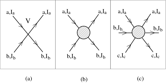
Figure 6: Feynman diagram representation of the interactions in Eqs. (69) and (79).

The quartic interactions of topological origin described by the contributions to $S^{1}_{\rm matter,CG}$ of Eq. (79) in which the fields $\boldsymbol{A}^{a}$ are coupled to the currents $\boldsymbol{J}^{a}$, correspond to the four-vertex of Fig. 6-(b). The sextic interactions, also of topological origin, consisting in the terms in $S^{1}_{\rm matter,CG}$ proportional to $(\boldsymbol{A}^{a})^{2}$, are displayed in Fig. 6-(c). Let us note that in both the four-vertex and the six-vertex of Figs. 6-(b) and 6-(c) the external legs depart from a solid circle. This circle symbolizes the fact that these vertices contain non-perturbative contributions coming from the path integral summation over the field $B_{\mu}^{ab}$ and $C_{\mu}^{ab}$. The strengths $g_{4}$ and $g_{6}$ of the quartic and sextic interactions of topological origin are respectively proportional to:

$$g_{4}\sim\frac{\lambda_{ab}}{8\pi^{2}}\qquad\qquad g_{6}\sim\frac{\lambda_{ab}\lambda_{ac}}{16\pi^{4}}$$ (83)

As it is clear from Eq. (16), the $\lambda_{ab}$’s are Fourier coefficients varying in the interval $(-\infty,+\infty)$. For this reason, $g_{4}$ and $g_{6}$ cannot be considered as real coupling constant. However, the parameters $\lambda_{ab}$ may be interpreted as chemical potentials that specify how easy is the linking of two trajectories $\Gamma_{a}$ and $\Gamma_{b}$. To small values of $\lambda_{ab}$ correspond big values of the linking number $m_{ab}$ and viceversa.

An important feature of the model described in Eqs. (77) and (78) is that the interactions of topological origin have sextic interactions, in which the monomers of three different loops are involved. The appearance of three-body forces was up to now not supposed to be possible in the case of topological constraints imposed using the Gauss linking number. As a matter of fact, this link invariant controls only the linking between pairs of polymer rings. In the case $N=2$, in which we have just two loops, these three-body interactions are suppressed as showed in Ref. [53], because they vanish when the limit in which the numbers of replicas $n_{a,I_{a}}$ approach zero is performed in the probability function of Eq. (77). However, not all diagrams with three-body interactions disappear when $N>2$. An example of nontrivial contribution in which interactions of three monomers are taking place is shown in Fig. 7.

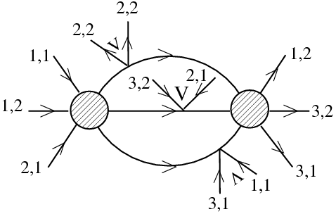
Figure 7: Example of a process in which the three body interactions of topological origin do not vanish in the zero replicas limit $n_{a,I_{a}}\to 0$ appearing in Eq. (77). The process describes the interaction of the subtrajectories $\Gamma_{a,I_{a}}$, $a=1,2,3$, $I_{a}=1,2$ forming a $6-$plat in which three loops $\Gamma_{1},\Gamma_{2},\Gamma_{3}$ are linked together.

Another characteristic of the model describing the statistical mechanics of $2s-$plats introduced here is the existence of vortex solutions of the equations that minimize the energy of the static field configurations. An example of such solutions will be presented in the next Section in the case $N=2$.

6 Self-dual solutions of the two-polymer problem

In this Section we restrict ourselves for simplicity to $4-$plats. Moreover, the non-topological interactions contained in $S^{2}_{\rm matter}$ will be ignored. We will also suppose that the replica numbers are independent of $I_{a}$, i.e.:

$$\vec{\Psi}(\boldsymbol{x},t)=(\psi^{1}_{a,I_{a}}(\boldsymbol{x},t),\ldots,\psi^{n_{a}}_{a,I_{a}}(\boldsymbol{x},t))\qquad a=1,2\mbox{ and }I_{a}=1,2$$ (84)

$$\vec{\Psi}^{\ast}(\boldsymbol{x},t)=(\psi^{1\ast}_{a,I_{a}}(\boldsymbol{x},t),\ldots,\psi^{\ast n_{a}}_{a,I_{a}}(\boldsymbol{x},t))\qquad a=1,2\mbox{ and }I_{a}=1,2.$$ (85)

In Eqs. (61) and (62) each pair of complex fields $\vec{\Psi}^{*}_{a,I_{a}},\vec{\Psi}_{a,I_{a}}$ had a separate replica index $n_{a,I_{a}}$, but it is easy to check that $I_{a}-$independent replica indexes are possible too without jeopardizing the passage to field theory and in particular the calculations made in Section 4. The partition function of a $4-$plat formed by two linked polymers is obtained by putting $N=2$ and $s_{1}=s_{2}=1$ in the general partition function of a $2s-$plat given in Eq. (77). Accordingly, the action $S_{\rm matter,CG}$ in Eq. (78) in this particular case becomes

$$S_{\rm matter,CG} = \int_{\tau_{1,0}}^{\tau_{1,1}}\!dt\int\!d^{2}\boldsymbol{x}\Bigg{\{}\vec{\Psi}_{1,1}^{*}\left[\frac{\partial}{\partial t}-\frac{1}{4g_{1,1}}\boldsymbol{D}^{2}\left(-\lambda_{12},\boldsymbol{B}^{12}\right)\right]\vec{\Psi}_{1,1}$$ (86)

$$+ \vec{\Psi}_{1,2}^{*}\left[\frac{\partial}{\partial t}-\frac{1}{4g_{1,2}}\boldsymbol{D}^{2}\left(\lambda_{12},\boldsymbol{B}^{12}\right)\right]\vec{\Psi}_{1,2}\Bigg{\}}$$

$$+ \int_{\tau_{2,0}}^{\tau_{2,1}}\!dt\int d^{2}\boldsymbol{x}\vec{\Psi}_{2,1}^{*}\Bigg{\{}\left[\frac{\partial}{\partial t}-\frac{1}{4g_{2,1}}\boldsymbol{D}^{2}\left(-\frac{\kappa}{8\pi^{2}},\boldsymbol{C}^{12}\right)\right]\vec{\Psi}_{2,1}$$

$$+ \vec{\Psi}_{2,2}^{*}\left[\frac{\partial}{\partial t}-\frac{1}{4g_{2,2}}\boldsymbol{D}^{2}\left(\frac{\kappa}{8\pi^{2}},\boldsymbol{C}^{12}\right)\right]\vec{\Psi}_{2,2}\Bigg{\}}.$$

In the above equation $\boldsymbol{D}$ denotes the covariant derivatives, which are of two types depending if they are defined with respect to the field $\boldsymbol{B}^{12}$ or to the field $\boldsymbol{C}^{12}$:

$$\boldsymbol{D}(\pm\lambda_{12},\boldsymbol{B}^{12})=\boldsymbol{\nabla}\pm i\lambda_{12}\boldsymbol{B}^{12}\qquad\qquad\boldsymbol{D}\left(\pm\frac{\kappa}{8\pi^{2}},\boldsymbol{C}^{12}\right)=\boldsymbol{\nabla}\pm i\frac{\kappa}{8\pi^{2}}\boldsymbol{C}^{12}.$$ (87)

As mentioned at the end of the previous Section, the fields $\boldsymbol{B}^{12}$ and $\boldsymbol{C}^{12}$ are not independent degrees of freedom, because they are fully determined by the constraints (73)–(76). In the present case $N=2$, $s_{1}=s_{2}=2$, the required conditions are:

$$\epsilon^{ij}\partial_{i}B_{j}^{12} = -\frac{1}{2\pi}\left(|\vec{\Psi}_{21}|^{2}+|\vec{\Psi}_{22}|^{2}\right)\theta(\tau_{2,1}-t)\theta(t-\tau_{2,0})$$ (88)

$$\epsilon^{ij}\partial_{i}C_{j}^{12} = -\frac{4\pi\lambda_{12}}{\kappa}\left(|\vec{\Psi}_{11}|^{2}+|\vec{\Psi}_{12}|^{2}\right)\theta(\tau_{1,1}-t)\theta(t-\tau_{1,0}).$$ (89)

We will consider now the static field configurations that minimize the action $S_{\rm matter,CG}$ of Eq. (86). From Ref. [30] it is known that this action admits self-dual solutions in the case in which the parameters $g_{a,I_{a}}$, $a=1,2$ and $I_{a}=1,2$ are all equal. To this purpose, for any constant $\gamma$ and gauge field $\boldsymbol{a}$ we define the new covariant derivatives $D_{\pm}(\gamma,\boldsymbol{a})$:

$$D_{\pm}(\gamma,\boldsymbol{a})=D_{1}(\gamma,\boldsymbol{a})\pm iD_{2}(\gamma,\boldsymbol{a})$$ (90)

where $D_{1}$ and $D_{2}$ denote the first and second components of the covariant derivative $\boldsymbol{D}$. In terms of the $D_{\pm}$’s, the self-duality equations may be expressed as follows:

$$D_{+}\left(-\lambda_{12},\boldsymbol{B}^{12}\right)\psi_{1,1}^{n_{1}} = 0$$ (91)

$$D_{+}\left(\lambda_{12},\boldsymbol{B}^{12}\right)\psi_{1,2}^{n_{1}} = 0$$ (92)

$$D_{-}\left(-\frac{\kappa}{8\pi^{2}},\boldsymbol{C}^{12}\right)\psi_{2,1}^{n_{2}} = 0$$ (93)

$$D_{-}\left(\frac{\kappa}{8\pi^{2}},\boldsymbol{C}^{12}\right)\psi_{2,2}^{n_{2}} = 0.$$ (94)

We notice in the constraints (88) and (89) the cumbersome presence of the Heaviside $\theta-$functions. They are required in order to take into account the fact that the heights of the points belonging to the subtrajectories $\Gamma_{a,I_{a}}$ are only partially overlapping. As a consequence, to avoid complications, we will assume that $\tau_{1,0}=\tau_{2,0}=\tau_{0}$ and $\tau_{1,1}=\tau_{2,1}=\tau_{1}$, i.e. all subtrajectories will start and end at the same height. In this way the Heaviside $\theta-$functions are no longer needed. Moreover, we will restrict ourselves to replica symmetric solutions by putting:

$$\psi^{1}_{1,I_{1}}=\cdots=\psi_{1,I_{1}}^{n_{1}} = \psi_{1,I_{1}}\quad\mbox{for}\quad I_{1}=1,2$$

$$\psi_{2,I_{2}}^{1}=\cdots=\psi_{2,I_{2}}^{n_{2}} = \psi_{2,I_{2}}\quad\mbox{for}\quad I_{2}=1,2.$$ (95)

After these simplifications, the self-duality conditions (91)–(94) and the constraints (88) and (89) become:

$$\left[\partial_{1}-i\lambda_{12}B_{1}^{12}+i\left(\partial_{2}-i\lambda_{12}B_{2}^{12}\right)\right]\psi_{1,1} = 0$$ (96)

$$\left[\partial_{1}+i\lambda_{12}B_{1}^{12}+i\left(\partial_{2}+i\lambda_{12}B_{2}^{12}\right)\right]\psi_{1,2} = 0$$ (97)

$$\left[\partial_{1}-\frac{i\kappa}{8\pi^{2}}C_{1}^{12}-i\left(\partial_{2}-\frac{i\kappa}{8\pi^{2}}C_{2}^{12}\right)\right]\psi_{2,1} = 0$$ (98)

$$\left[\partial_{1}+\frac{i\kappa}{8\pi^{2}}C_{1}^{12}-i\left(\partial_{2}+\frac{i\kappa}{8\pi^{2}}C_{2}^{12}\right)\right]\psi_{2,2} = 0$$ (99)

and

$$\epsilon^{ij}\partial_{i}B_{j}^{12} = -\frac{1}{2\pi}n_{2}\left(|\psi_{2,1}|^{2}+|\psi_{2,2}|^{2}\right)$$ (100)

$$\epsilon^{ij}\partial_{i}C_{j}^{12} = -\frac{4n_{1}\pi\lambda_{12}}{\kappa}\left(|\psi_{1,1}|^{2}+|\psi_{1,2}|^{2}\right).$$ (101)

At this point we pass to polar coordinates by performing the transformations:

$$\psi_{a,I_{a}}={\rm e}^{i\omega_{a,I_{a}}}\rho_{a,I_{a}}^{1/2}.$$ (102)

After the above change of variables in Eqs. (96–101) and separating the real and imaginary parts, we obtain:

$$\partial_{1}\omega_{1,1}-\lambda_{12}B_{1}^{12}+\frac{1}{2}\partial_{2}\log\rho_{1,1} = 0$$ (103)

$$-\partial_{2}\omega_{1,1}+\lambda_{12}B_{2}^{12}+\frac{1}{2}\partial_{1}\log\rho_{1,1} = 0$$ (104)

$$\partial_{1}\omega_{1,2}+\lambda_{12}B_{1}^{12}+\frac{1}{2}\partial_{2}\log\rho_{1,2} = 0$$ (105)

$$-\partial_{2}\omega_{1,2}-\lambda_{12}B_{2}^{12}+\frac{1}{2}\partial_{1}\log\rho_{1,2} = 0$$ (106)

$$\partial_{1}\omega_{2,1}-\frac{\kappa}{8\pi^{2}}C_{1}^{12}-\frac{1}{2}\partial_{2}\log\rho_{2,1} = 0$$ (107)

$$\partial_{2}\omega_{2,1}-\frac{\kappa}{8\pi^{2}}C_{2}^{12}+\frac{1}{2}\partial_{1}\log\rho_{2,1} = 0$$ (108)

$$\partial_{1}\omega_{2,2}+\frac{\kappa}{8\pi^{2}}C_{1}^{12}-\frac{1}{2}\partial_{2}\log\rho_{2,2} = 0$$ (109)

$$\partial_{2}\omega_{2,2}+\frac{\kappa}{8\pi^{2}}C_{2}^{12}+\frac{1}{2}\partial_{1}\log\rho_{2,2} = 0$$ (110)

$$\epsilon^{ij}\partial_{i}B_{j} = -\frac{1}{2\pi}n_{2}\left(\rho_{2,1}+\rho_{2,2}\right)$$ (111)

$$\epsilon^{ij}\partial_{i}C_{j} = -\frac{4n_{1}\pi\lambda_{12}}{\kappa}\left(\rho_{1,1}+\rho_{1,2}\right).$$ (112)

To solve equations (103)–(110) with respect to the unknowns $\omega_{a,I_{a}}$ and $\rho_{a,I_{a}}$, we proceed as follows. First of all, we isolate from Eq. (103) and Eq. (105) the same quantity $\lambda_{12}B_{1}^{12}$. By requiring that the expressions of $\lambda_{12}B_{1}^{12}$ provided by Eqs. (103) and (105) are equal, we obtain the consistency condition

$$\partial_{1}\omega_{1,1}+\frac{1}{2}\partial_{2}\log\rho_{1,1}=-\partial_{1}\omega_{1,2}-\frac{1}{2}\partial_{2}\log\rho_{1,2}$$ (113)

A possible solution of Eq. (113) is

$$\omega_{1,1}=-\omega_{1,2}\quad\mbox{and}\quad\rho_{1,1}=\frac{A_{1}}{\rho_{1,2}}$$ (114)

where $A_{1}$ is at most a function of $x^{1}$. As well, we require that the two different expressions of the quantity $\lambda_{12}B_{2}^{12}$ obtained from Eqs. (104) and (106) are equal. On this way one obtains a condition analogous to (113), which may be solved by applying the ansatz (114) and additionally requiring that $A_{1}$ is a constant. In a similar way, it is possible to extract from equations (107–110) the conditions:

$$\omega_{2,1}=-\omega_{2,2}\quad\mbox{and}\quad\rho_{2,1}=\frac{A_{2}}{\rho_{2,2}}$$ (115)

with $A_{2}$ being a constant.

Thanks to Eqs. (114) and (115), the number of unknowns to be computed is reduced. For instance, if we choose as independent degrees of freedom $\omega_{1,1},\omega_{2,1},\rho_{1,1}$ and $\rho_{2,1}$, the remaining classical field configurations $\omega_{1,2},\omega_{2,2},\rho_{1,2}$ and $\rho_{2,2}$ can be derived using such equations. As a consequence, the system of equations (103)–(112) reduces to:

$$\lambda_{12}B_{1}^{12} = \partial_{1}\omega_{1,1}+\frac{1}{2}\partial_{2}\log\rho_{1,1}$$ (116)

$$\lambda_{12}B_{2}^{12} = \partial_{2}\omega_{1,1}-\frac{1}{2}\partial_{1}\log\rho_{1,1}$$ (117)

$$\frac{\kappa}{8\pi^{2}}C_{1}^{12} = \partial_{1}\omega_{2,1}-\frac{1}{2}\partial_{2}\log\rho_{2,1}$$ (118)

$$\frac{\kappa}{8\pi^{2}}C_{2}^{12} = \partial_{2}\omega_{2,1}+\frac{1}{2}\partial_{1}\log\rho_{2,1}$$ (119)

$$\partial_{1}B_{2}^{12}-\partial_{2}B_{1}^{12} = -\frac{1}{2\pi}n_{2}\left(\rho_{2,1}+\frac{A_{2}}{\rho_{2,1}}\right)$$ (120)

$$\partial_{1}C_{2}^{12}-\partial_{2}C_{1}^{12} = -\frac{4n_{1}\pi\lambda_{12}}{\kappa}\left(\rho_{1,1}+\frac{A_{1}}{\rho_{1,1}}\right)$$ (121)

where we have used the fact that $\epsilon^{ij}\partial_{i}B_{j}=\partial_{1}B_{2}^{12}-\partial_{2}B_{1}^{12}$ and $\epsilon^{ij}\partial_{i}C_{j}=\partial_{1}C_{2}^{12}-\partial_{2}C_{1}^{12}$. Eqs. (116)–(121) contain the unknowns $\omega_{1,1},\omega_{2,1},\rho_{1,1}$ and $\rho_{2,1}$ that will be determined below.

By subtracting term by term the two equations resulting from the derivation of Eqs. (116) and (117) with respect to the variables $x^{2}$ and $x^{1}$ respectively, we obtain as an upshot the relation:

$$\lambda_{12}\left(\partial_{1}B_{2}^{12}-\partial_{2}B_{1}^{12}\right)=\partial_{1}\partial_{2}\omega_{1,1}-\partial_{2}\partial_{1}\omega_{1,1}-\frac{1}{2}\Delta\log\rho_{1,1}$$ (122)

with $\Delta=\partial_{1}^{2}+\partial_{2}^{2}$ being the two-dimensional Laplacian.
Assuming that $\omega_{1,1}$ is a regular function satisfying the relation

$$\partial_{1}\partial_{2}\omega_{1,1}-\partial_{2}\partial_{1}\omega_{1,1}=0$$ (123)

Eq. (122) becomes:

$$\lambda_{12}\left(\partial_{1}B_{2}^{12}-\partial_{2}B_{1}^{12}\right)=-\frac{1}{2}\Delta\log\rho_{1,1}.$$ (124)

An analogous identity can be derived starting from Eqs. (118) and (119):

$$\frac{\kappa}{4\pi^{2}}\left(\partial_{1}C_{2}^{12}-\partial_{2}C_{1}^{12}\right)=\Delta\log\rho_{2,1}.$$ (125)

The compatibility of (124) and (125) with the constraints (120) and (121) respectively leads to the following conditions between $\rho_{1,1}$ and $\rho_{2,1}$:

$$\Delta\log\rho_{1,1} = \frac{\lambda_{12}n_{2}}{\pi}\left(\frac{A_{2}}{\rho_{2,1}}+\rho_{2,1}\right)$$ (126)

$$\Delta\log\rho_{2,1} = -\frac{\lambda_{12}n_{1}}{\pi}\left(\rho_{1,1}+\frac{A_{1}}{\rho_{1,1}}\right).$$ (127)

The fact that $\rho_{1,1}$ and $\rho_{2,1}$ appear in a symmetric way in Eqs. (126) and (127), suggests the following ansatz:

$$\rho_{2,1}=\frac{A_{3}}{\rho_{1,1}}$$ (128)

with $A_{3}$ being a constant. It is easy to check that with this ansatz Eqs. (126) and (127) remain compatible provided:

$$\frac{A_{2}}{A_{3}}=\frac{n_{1}}{n_{2}}\quad\mbox{and}\quad\frac{A_{3}}{A_{1}}=\frac{n_{1}}{n_{2}}.$$ (129)

We choose $A_{1}$ to be the independent constant, while $A_{2}$ and $A_{3}$ are constrained by Eq. (129) to be dependent on $A_{1}$:

$$A_{2}=\left(\frac{n_{1}}{n_{2}}\right)^{2}A_{1}\qquad A_{3}=\frac{n_{1}}{n_{2}}A_{1}.$$ (130)

We are now left only with the task of computing the explicit expression of $\rho_{1,1}$. This may be obtained by solving the equation:

$$\Delta\log{\rho_{1,1}}=\frac{\lambda_{12}n_{1}}{\pi}\left(\frac{A_{1}}{\rho_{1,1}}+\rho_{1,1}\right)$$ (131)

The other quantities $\rho_{2,1}$, $\rho_{1,2}$ and $\rho_{2,2}$ can be derived using the relations (128), (114) and (115) respectively. Eq. (131) may be cast in a more familiar form by putting: $\eta=\ln\left(\frac{\rho_{1,1}}{\sqrt{A_{1}}}\right)$. After this substitution, Eq. (131) becomes the Euclidean cosh–Gordon equation with respect to $\eta$:

$$\Delta\eta=\frac{2\lambda_{12}n_{1}}{\pi}\sqrt{A_{1}}\cosh\eta$$ (132)

Next, it is possible to determine the magnetic fields $\boldsymbol{B}^{12}$ and $\boldsymbol{C}^{12}$ from Eqs. (120) and (121). In the Coulomb gauge, in fact, the two-dimensional vector potentials $\boldsymbol{B}^{12}$ and $\boldsymbol{C}^{12}$ can be represented using two scalar fields $b^{12}$ and $c^{12}$ as follows (see also Eq. (30)):

$$\boldsymbol{B}^{12}=(-\partial_{2}b^{12},\partial_{1}b^{12})\qquad\boldsymbol{C}^{12}=(-\partial_{2}c^{12},\partial_{1}c^{12})$$ (133)

Performing the above substitutions in Eqs. (120) and (121), it turns out that $b^{12}$ and $c^{12}$ satisfy the relations:

$$\Delta b^{12}=-\frac{n_{1}}{2\pi}(\rho_{1,1}+\frac{A_{1}}{\rho_{1,1}})$$ (134)

$$\Delta c^{12}=-\frac{4n_{1}\pi\lambda_{12}}{\kappa}(\rho_{1,1}+\frac{A_{1}}{\rho_{1,1}})$$ (135)

The solution of Eqs. (134) and (135) can be easily derived with the help of the method of the Green functions once the expression of $\rho_{1,1}$ is known. Finally, the phases $\omega_{1,1}$, $\omega_{1,2}$, $\omega_{2,1}$ and $\omega_{2,2}$ are computed using Eqs. (116)–(119). In fact, remembering that we assumed that $\omega_{1,1}=-\omega_{1,2}$ and $\omega_{2,1}=-\omega_{2,2}$ in (114) and (115) respectively, we have only to determine $\omega_{1,1}$ and $\omega_{2,1}$. By deriving Eq. (116) with respect to $x^{1}$ and Eq. (117) with respect to $x^{2}$, we obtain:

$$\lambda_{12}\partial_{1}B_{1}^{12} = \partial_{1}^{2}\omega_{1,1}+\frac{1}{2}\partial_{1}\partial_{2}\log{\rho_{1,1}}$$

$$\lambda_{12}\partial_{2}B_{2}^{12} = \partial_{2}^{2}\omega_{1,1}-\frac{1}{2}\partial_{2}\partial_{1}\log{\rho_{1,1}}$$ (136)

On the other side, by adding term by term the above two equations and using the fact that in the Coulomb gauge the magnetic field $\boldsymbol{B}^{12}$ is completely transverse, it is possible to show that:

$$\Delta\omega_{1,1}=0$$ (137)

Proceeding in a similar way with Eq. (118) and (119) it is possible to derive also the relation satisfied by $\omega_{2,1}$:

$$\Delta\omega_{2,1}=0$$ (138)

7 Conclusions

In this work a $2s-$plat composed by $N$ polymers forming a nontrivial link has been considered. The nontrivial interactions and the topological constraints make the energy density of the system complicated and nonlocal, but it can be simplified with the introduction of auxiliary fields. The final model which we obtain is a standard field theory involving a set of complex scalar fields with sextic interactions at most. This model allows also some phenomenological predictions that were a priori not obvious and that will be summarized below.

1. In the case of a $4-$plat, it has been shown in [30] with the help of a Bogomol’nyi tranformation that, after eliminating the fields $B_{\mu}^{ab}$ and $C_{\mu}^{ab}$, the topological constraints imposed with the Gauss linking number are responsible for quartic interaction terms in the Hamiltonian of the system. In the particular case in which the two-body potential of the non-topological interactions is given by Eq. (41), these quartic terms are exactly of the same form of those contained in the action (69). Here we have seen in the more general case of a $2s-$plat and an arbitrary two-body potential $V(\boldsymbol{r}_{2}-\boldsymbol{r}_{1})$ how the interactions arising due to the presence of the constraints interphere with the non-topological interactions of Eq. (37). For example, from Eq. (64) it is possible to realize that in the action $S_{part}(\vec{\Psi}_{a,I_{a}}^{\ast},\vec{\Psi}_{a,I_{a}})$ the third components of the BF-fields can be absorbed by the fields $\varphi_{a,I_{a}}$ after a shift. Since the BF-fields are related to the topological constraints and the fields $\varphi_{a,I_{a}}$ are propagating the non-topological forces, this hints to a strong interplay between the topological and non-topological interactions. Let us note that the effect of the forces of topological origin may result both in a reciprocal attraction or repulsion between the monomers, while the short range two-body potential (41), corresponding to the case in which the polymers are immersed in a solution, can only be attractive if $V_{0}<0$ or repulsive if $V_{0}>0$.

2. The field theoretical model of polymeric $2s-$plats defined by Eqs. (77)–(82) shows that three-body forces become relevant in a system of $N$ polymers linked together in which the topological constraints are imposed by means of the Gauss linking number. These three-body forces have been represented in the form of a Feynman diagram in Fig. 6-(c) and are described in Section 5. An example of process in which there are interactions between three monomers at once has been shown in Fig. 7. The existence of three-body interactions acting on the monomers was not predicted by previous calculations. This is probably because only the case $N=2$ has been mainly treated so far. When $N=2$, it turns out that the contribution of sextic interactions terms in the action of Eq. (79), which are responsible for the presence of the three-body forces, vanishes in the zero replica limit. Besides, the appearance of three-body forces is not trivial and not easy to be predicted, because the Gauss linking number involves only interactions between pairs of monomers.

3. By using the splitting procedure presented in Section 2 and thanks to the introduction of auxiliary fields, the problem of the statistical mechanics of a $2s-$plat has been mapped into the dynamics of a system in which quasiparticles of different kinds are mixed together. In Ref. [30] it has been shown that systems of this type admit vortex solutions. Out of the self-duality regime, vortex magnetic lines associated with quasi-particles of different kind can repel or attract themselves. After a particular choice of the parameters of the theory, in which the coefficients $g_{a,I_{a}}$, $a=1,2$ and $I_{a}=1,2$ are all equal, a self-dual point is reached in which attractive and repulsive forces balance themselves and disappear. A similar phenomenon, but in a different model, has been recently found in Ref. [54]. In this work, the self-dual vortex conformations have been computed exactly and explicitly up to the solution of a cosh-Gordon equation.

The topological properties of the link formed by the $2s-$plat have been described here by using the Gauss linking invariant, which is related to the abelian BF-model of Eq. (44). We have seen in Appendix B how the topological constraints are fixed when the BF-model is quantized in the Coulomb gauge. In this gauge are counted the winding numbers of all possible pairs of paths formed by the subtrajectories $\Gamma_{a,I_{a}}$ belonging to a loop $\Gamma_{a}$ and the subtrajectories $\Gamma_{b,I_{b}}$ belonging to another loop $\Gamma_{b}$. The sum of all these winding numbers is an integer multiple of $2\pi$, where the integer is equal to the half of the number of left and right crossings of the two oriented trajectories $\Gamma_{a}$ and $\Gamma_{b}$. This number is independent on the way in which the trajectories are projected on a plane and provides a well known alternative definition of the Gauss linking number. In this way, also in the Coulomb gauge the condition that the Gauss linking number of $\Gamma_{a}$ and $\Gamma_{b}$ should be equal to some value $m_{ab}$ is realized. While abelian anyon field theories like those of Eq. (44) may be significant in quantum computing [55], it is rather nonabelian statistics that plays the main role in this kind of applications. Despite its limitations, when the Gauss linking number is applied to a $2s-$plat configuration, which cannot be destroyed because the $2s$ points of maxima and minima are kept fixed, some of the nonabelian features of the system are certainly captured. As a matter of fact, in the case of $2s-$plats the capabilities of the Gauss linking number to distinguish the changes of topology are enhanced. The reason is the synergy between the constraints imposed by the Gauss linking number and those imposed by the fact that the polymer system cannot escape the set of conformations allowed in a $2s-$plat. Indeed, since the end points of the subtrajectories $\Gamma_{a,I_{a}}$ and $\Gamma_{b,I_{b}}$ are fixed, also the winding number between two different subtrajectories is fixed. Due to the constraints imposed by the linking number, allowed are only those topology changes for which an amount of the winding angle of two subtrajectories is transferred in units of $2\pi$ to the winding angle of another pair of subtrajectories. Moreover, the number of subtrajectories is fixed to be equal to $2s$. As a consequence, at least in the particular case of $2s-$plats, it is possible to overcome the limitations of the Gauss linking number. As mentioned in the Introduction, if we start from an unlink consisting of a $4-$plat, the system will never be able to attain the configuration of a Whitehead link and viceversa, a $6-$plat Whitehead link cannot turn into a $4-$plat. Moreover, in a forthcoming publication we will show how the present formalism can be applied to include the treatment of links without the limitations of the Gauss linking number and even to the case of nontrivial knots. This will pave the way to the treatment of polymer knots or links constructed from tangles. Polymers of this kind are relevant in biochemistry because nontrivial knot configurations appearing as a major pattern in DNA rings are mostly in the form of tangles [11].

8 Acknowledgments

F. Ferrari would like to thank E. Szuszkiewicz for pointing out Ref. [56] and inspiring the present work. We wish to thank heartily also M. Pyrka, V. G. Rostiashvili and T. A. Vilgis for fruitful discussions. The simulations reported in this work were performed in part using the HPC cluster HAL9000 of the Computing Centre of the Faculty of Mathematics and Physics at the University of Szczecin.

Appendix A The length $L$ of a directed polymer as a function of the height

In this Appendix we consider the partition function

$${\cal Z}=\int\!{\cal D}\boldsymbol{r}(z)e^{-S}$$ (139)

where $S$ is the action of the free open polymer, whose trajectory $\Gamma$ is parametrized by means of the height $z$ defined in some interval $[\tau_{0},\tau_{1}]$:

$$S=g\int_{\tau_{0}}^{\tau_{1}}dz\left|\frac{d\boldsymbol{r}}{dz}\right|^{2}$$ (140)

We want now to determine how the total length of the curve $\Gamma$ depends on the constant parameter $g$. To understand what we mean by that, let us consider the standard case of an ideal chain whose trajectory is parametrized with the help of the arc-length $\sigma$. We denote with $a$ the average statistical length (Kuhn length) of the $N$ segments composing the polymer. In the limit of large $N$ and small $a$ such that the product $Na$ is constant, the total length $L$ of the polymer satisfies the relation

$$L=Na$$ (141)

We wish to obtain a similar identity connecting $L$ with $N$ and $g$ in the present situation, which is somewhat different. To this purpose, we first dicretize the interval of integration $[\tau_{0},\tau_{1}]$ splitting it into $N$ small segments of length:

$$\Delta z=\frac{\tau_{1}-\tau_{0}}{N}$$ (142)

As a consequence, we may approximate the action as follows:

$$S\sim g\sum_{w=1}^{N}\left|\frac{\Delta\boldsymbol{r}_{w}}{\Delta z}\right|^{2}\Delta z$$ (143)

where the symbol $\Delta\boldsymbol{r}_{w}$ means

$$\Delta\boldsymbol{r}_{w}=\boldsymbol{r}_{w+1}-\boldsymbol{r}_{w}$$ (144)

and

$$\boldsymbol{r}_{w}=\boldsymbol{r}(\tau_{0}+w\Delta z)$$ (145)

The discretized partition function becomes thus the partition function of a random chain composed by $N$ segments:

$${\cal Z}_{disc}=\int\!\prod_{w=1}^{N}d\boldsymbol{r}_{w}e^{-\sum\limits_{w=1}^{N}g\frac{|\Delta\boldsymbol{r}_{w}|^{2}}{\Delta z}}$$ (146)

Using simple trigonometric arguments it is easy to realize that the length of each segment is:

$$\Delta L=\sqrt{|\Delta\boldsymbol{r}_{w}|^{2}+(\Delta z)^{2}}$$ (147)

This is of course an average length, dictated by the fact that, from Eq. (146), the values of $|\Delta\boldsymbol{r}_{w}|$ should be gaussianly distributed around the point:

$$|\Delta\boldsymbol{r}_{w}|^{2}=\frac{\Delta z}{g}$$ (148)

In the limit $\Delta z\rightarrow 0$, the distribution of length of $\Delta\boldsymbol{r}_{w}$ becomes the Dirac $\delta$-function:

$$\lim_{\Delta z\rightarrow 0}\frac{1}{2}\sqrt{\frac{g}{\Delta z}}e^{-g|\Delta\boldsymbol{r}_{w}|^{2}/\Delta z}\sim\delta\left(|\Delta\boldsymbol{r}_{w}|-\sqrt{\frac{\Delta z}{g}}\right)$$ (149)

If $N$ is large enough, we can therefore conclude that the total length of the chain $\Gamma$ is:

$$L\sim N\Delta L=N\sqrt{\frac{\Delta z}{g}+(\Delta z)^{2}}$$ (150)

Since $N\Delta z=\tau_{1}-\tau_{0}$, we get:

$$L^{2}=|\tau_{1}-\tau_{0}|^{2}+\frac{N(\tau_{1}-\tau_{0})}{g}$$ (151)

In the limit $N\rightarrow\infty$, while keeping the ratio $\frac{N}{g}$ finite, Eq. (151) becomes the desired relation between the length of $\Gamma$ and $g$ which replaces Eq. (141).

Appendix B The expression of the Gauss linking invariant in the Coulomb gauge

To fix the ideas, we will study here the particular case of a $4-$plat. In the partition function (43) we isolate only the terms in which the BF fields appear, because the other contributions are not connected to topological constraints and thus are not relevant. As a consequence, we have just to compute the following partition function:

$${\cal Z}_{BF,CG}(\lambda)=\int\!{\cal D}B_{\mu}{\cal D}C_{\mu}e^{-iS_{BF,CG}-S_{top}}$$ (152)

where the BF action in the Coulomb gauge $S_{BF,CG}$ has been already defined in Eq. (29) and $S_{top}$ has been given in Eq. (45). In the case of a $4-$plat, $S_{top}$ becomes:

$$S_{top} = i\lambda\int_{\tau_{1,0}}^{\tau_{1,1}}dt\left[\frac{dx_{1,1}^{\mu}(t)}{dt}B_{\mu}(\boldsymbol{r}_{1,1}(t),t)-\frac{dx_{1,2}^{\mu}(t)}{dt}B_{\mu}(\boldsymbol{r}_{1,2}(t),t)\right]$$ (153)

$$+ \frac{i\kappa}{8\pi^{2}}\int_{\tau_{2,0}}^{\tau_{2,1}}dt\left[\frac{dx_{2,1}^{\mu}(t)}{dt}C_{\mu}(\boldsymbol{r}_{2,1}(t),t)-\frac{dx_{2,2}^{\mu}(t)}{dt}C_{\mu}(\boldsymbol{r}_{2,2}(t),t)\right]$$

where we recall that $x_{a,I}^{\mu}(t)=(\boldsymbol{r}_{a,I}(t),t)$, $a=1,2$, $I=1,2$. For simplicity of the notation, in this Appendix we use $\lambda$ instead of $\lambda_{12}$. Using the Chern-Simons propagator of Eqs. (33)-(34), it is easy to evaluate the path integral over the gauge fields in Eq. (152). The result, after two simple Gaussian integrations, is:

$$Z_{BF,CG}(\lambda)=\exp{\left\{\frac{i\lambda}{2\pi}\sum_{I,J=1}^{2}(-1)^{I+J-2}\epsilon_{ij}\int_{\tau_{0}}^{\tau_{1}}d(x_{1,I}^{i}(t)-x_{2,J}^{i}(t))\frac{(x_{1,I}^{j}(t)-x_{2,J}^{j}(t))}{\left|\boldsymbol{r}_{1,I}(t)-\boldsymbol{r}_{2,J}(t)\right|^{2}}\right\}}$$ (154)

In the above equation we have put for simplicity:

$$\tau_{0} = \max[\tau_{1,0},\tau_{2,0}]$$

$$\tau_{1} = \min[\tau_{1,1},\tau_{2,1}]$$ (155)

For instance, if the polymer configurations are as in Fig. 8, we have that $\tau_{0}=\tau_{1,0}$ and $\tau_{1}=\tau_{2,1}$.

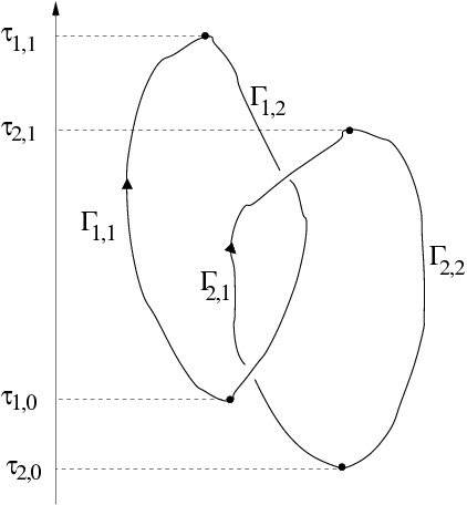
Figure 8: Example of configuration of a $4-$plat.

Moreover, we remember that in our notation $\boldsymbol{r}_{a,I}(t)=(x_{a,I}^{1}(t),x_{a,I}^{2}(t))$. Apparently, the elements of the trajectories $\Gamma_{1}$ and $\Gamma_{2}$ which lie below $\tau_{0}$ and above $\tau_{1}$ do not take the part in the topological interactions. Thus is due to the presence of the Dirac $\delta$-function $\delta(t-t^{\prime})$ in the components of the Chern-Simons propagator (33)-(34). However, we will see later that also the contributions of these missing parts are present in the expression of $Z_{BF,CG}(\lambda)$. In order to proceed, we notice that the exponent of the right hand side of Eq. (154) consists in a sum of integrals over the time $t$ of the kind:

$$D_{1,I;2,J}(\tau_{1})-D_{1,I;2,J}(\tau_{0})=\epsilon_{ij}\int_{\tau_{0}}^{\tau_{1}}d\left(x_{1,I}^{i}(t)-x_{2,J}^{i}(t)\right)\frac{(x_{1,I}^{j}(t)-x_{2,J}^{j}(t))}{\left|\boldsymbol{r}_{1,I}(t)-\boldsymbol{r}_{2,J}(t)\right|^{2}}$$ (156)

The above integrals can be computed exactly. It is in fact well known that the function $D_{1,I;2,J}(t)$ is the winding angle of the vector $\boldsymbol{r}_{1,I}(t)-\boldsymbol{r}_{2,J}(t)$ at time $t$:

$$D_{1,I;2,J}(t)=\arctan\left(\frac{x_{1,I}^{1}(t)-x_{2,J}^{1}(t)}{x_{1,I}^{2}(t)-x_{2,J}^{2}(t)}\right)$$ (157)

Thus, the quantity $D_{1,I;2,J}(\tau_{1})-D_{1,I;2,J}(\tau_{0})$ is a difference of winding angles which measures how many times the trajectory $\Gamma_{1,I}$ turns around the trajectory $\Gamma_{2,J}$ in the slice of time $\tau_{0}\leq t\leq\tau_{1}$. At this point, without any loss of generality, we suppose that the configurations of the curves $\Gamma_{1}$ and $\Gamma_{2}$ are such that the maxima and minima $\tau_{a,I}$ are ordered as follows:

$$\tau_{2,0}<\tau_{1,0}<\tau_{2,1}<\tau_{1,1}$$ (158)

As example of loop configurations that respect this ordering is given in Fig. 8. As a consequence, we have:

$$\tau_{0}=\tau_{1,0}\qquad\mbox{and}\qquad\tau_{1}=\tau_{2,1}$$ (159)

Now we notice that the logarithm of the gauge partition function ${\cal Z}_{BF,CG}(\lambda)$ in Eq. (154) contains a sum of differences of the winding angles defined in Eq. (157):

$$\frac{2\pi\log{{\cal Z}_{BF,CG}}(\lambda)}{i\lambda} = \left[D_{1,1;2,1}(\tau_{2,1})-D_{1,1;2,1}(\tau_{1,0})+D_{1,2;2,2}(\tau_{2,1})-D_{1,1;2,2}(\tau_{2,1})\right.$$ (160)

$$+ \left.D_{1,2;2,1}(\tau_{1,0})-D_{1,2;2,1}(\tau_{2,1})+D_{1,1;2,2}(\tau_{1,0})-D_{1,2;2,2}(\tau_{1,0})\right]$$

Further, assuming that the curves $\Gamma_{1}$ and $\Gamma_{2}$ are oriented as in Fig. 8. if we start from the minimum point at $\tau_{0}=\tau_{1,0}$, we can isolate in the right hand side of Eq. (160) the following four contributions:

1. In the time slice $\tau_{1,0}\leq t\leq\tau_{2,1}$ the angle which measures the winding of the trajectory $\Gamma_{1,1}$ around the trajectory $\Gamma_{2,1}$ is given by the difference $D_{1,1;2,1}(\tau_{2,1})-D_{1,1;2,1}(\tau_{1,0})$.

2. In the region $\tau_{2,1}\leq t\leq\tau_{1,1}$ only the trajectory $\Gamma_{1}$ continues to evolve, going first upwards with the subtrajectory $\Gamma_{1,1}$ and then downwards with $\Gamma_{1,2}$. After this evolution, the winding angle between the two trajectories $\Gamma_{1}$ and $\Gamma_{2}$ has changed by the quantity $D_{1,2;2,2}(\tau_{2,1})-D_{1,1;2,2}(\tau_{2,1})$.

3. Next, in the region $\tau_{2,1}\geq t\geq\tau_{1,0}$, the winding angle which measures how many times the subtrajectory $\Gamma_{1,2}$ winds up around $\Gamma_{2,2}$ is given by the difference $D_{1,2;2,1}(\tau_{1,0})-D_{1,2;2,1}(\tau_{2,1})$.

4. Finally, in the region $\tau_{1,0}\geq t\geq\tau_{2,0}$ only the second trajectory $\Gamma_{2}$ continues to evolve, going first downwards with the curve $\Gamma_{2,2}$ and then upwards with $\Gamma_{2,1}$. The net effect of this evolution is that the winding angle between $\Gamma_{1}$ and $\Gamma_{2}$ changes by the quantity $D_{1,1;2,2}(\tau_{1,0})-D_{1,2;2,2}(\tau_{1,0})$.

It is thus clear that the right hand side of Eq. (160), apart from a proportionality factor $i\lambda$, counts how many times the trajectory $\Gamma_{1}$ winds around the trajectory $\Gamma_{2}$. If we wish to identify the quantity in the right hand side of Eq. (160) with the Gauss linking number $\chi(\Gamma_{1},\Gamma_{2})$, we should check for consistency that it takes only integer values as the Gauss linking number does. Indeed, it is easy to see that, modulo $2\pi$, the following identities are holding:

$$D_{1,1;2,1}(\tau_{2,1}) = D_{1,1;2,2}(\tau_{2,1})$$

$$D_{1,1;2,2}(\tau_{1,0}) = D_{1,2;2,2}(\tau_{1,0})$$

$$D_{1,2;2,2}(\tau_{2,1}) = D_{1,2;2,1}(\tau_{2,1})$$

$$D_{1,1;2,1}(\tau_{1,0}) = D_{1,2;2,1}(\tau_{1,0})$$ (161)

For example, the first of the above equalities states that the angle formed by the vector $\boldsymbol{r}_{1,1}-\boldsymbol{r}_{2,1}$ connecting the subtrajectories $\Gamma_{1,1}$ and $\Gamma_{2,1}$ at the height $\tau_{2,1}$ is equal to the angle formed by the vector $\boldsymbol{r}_{1,1}-\boldsymbol{r}_{2,2}$ connecting the subtrajectories $\Gamma_{1,1}$ and $\Gamma_{2,2}$ at the same height. The reason of this identity is trivial: At that height, the subtrajectories $\Gamma_{2,1}$ and $\Gamma_{2,2}$ are connected together at the same point. Applying the above relations to Eq. (160), one may prove that:

$$\frac{2\pi\log{{\cal Z}_{BF,CG}}(\lambda)}{i\lambda}=0\qquad\qquad\mod 2\pi$$ (162)

As a consequence, we can write:

$${\cal Z}_{BF,CG}(\lambda)=e^{i\lambda\chi(\Gamma_{1},\Gamma_{2})}$$ (163)

where $\chi(\Gamma_{1},\Gamma_{2})$ is the Gauss linking number. Concluding, the above analysis shows that also in the Coulomb gauge the BF fields in the polymer partition function (43) fix the topological constraints (15) correctly, in full consistency with the results obtained in the covariant gauges. Of course this consistency was expected due to gauge invariance. Yet, it is interesting that, using the Coulomb gauge, one may express the Gauss linking number invariant in a way that is quite different from the usual form given in Eq. (14).

References

- [1] A. Yu. Grosberg, Phys.-Usp. 40 (1997), 12.
- [2] W. R. Taylor, Nature (London) 406 (2000), 916.
- [3] V. Katritch, J. Bednar, D. Michoud, R. G. Scharein, J. Dubochet, A. Stasiak, Nature 384 (1996), 142.
- [4] V. Katritch, W. K. Olson, P. Pieranski, J. Dubochet and A. Stasiak, Nature 388 (1997), 148.
- [5] M. A. Krasnow, A. Stasiak, S. J. Spengler, F. Dean, T. Koller and N. R. Cozzarelli, Nature 304 (1983), 559.
- [6] B. Laurie, V. Katritch, J. Dubochet and A. Stasiak, Biophys. J. 74 (1998), 2815.
- [7] J. I. Sułkowksa, P. Sułkowksa, P. Szymczak and M. Cieplak, Phys. Rev. Lett. 100 (2008), 058106.
- [8] J. F. Marko, Phys. Rev. E 79 (2009), 051905.
- [9] Z. Liu, E. L. Zechiedrich, and H. S. Chan, Biophys. J. 90 (2006), 2344.
- [10] S. A. Wasserman and N. R. Cozzarelli, Science 232 (1986), 951.
- [11] D. W. Sumners, Knot theory and DNA, in New Scientific Applications of Geometry and Topology, edited by D. W. Sumners, Proceedings of Symposia in Applied Mathematics, Vol. 45, American Mathematical Society, Providence, RI, (1992), 39.
- [12] A. V. Vologodski, A. V. Lukashin, M. D. Frank-Kamenetski and V. V. Anshelevich, Zh. Eksp. Teor. Fiz. 66 (1974), 2153; Sov. Phys. JETP 39 (1975), 1059; M. D. Frank-Kamenetskii, A. V. Lukashin and A. V. Vologodskii, Nature (London) 258 (1975), 398.
- [13] E. Orlandini, S. G. Whittington, Rev. Mod. Phys. 79 (2007), 611; C. Micheletti, D. Marenduzzo, and E. Orlandini, Phys. Rep. 504 (2011), 1.
- [14] S. D. Levene, C. Donahue, T. C. Boles and N. R. Cozzarelli, Biophys. J. 69 (1995), 1036.
- [15] T. Vettorel, A. Yu. Grosberg and K. Kremer, Phys. Biol. 6 (2009), 025013.
- [16] P. Virnau, Y. Kantor and M. Kardar, J. Am. Chem. Soc. 127 (43) (2005), 15102.
- [17] P. Pierański, S. Przybył and A. Stasiak, EPJ E 6 (2) (2001), 123.
- [18] J. Yan, M. O. Magnasco and J. F. Marko, Nature 401 (1999), 932.
- [19] J. Arsuaga, M. Vazquez, S. Trigueros, D. W. Sumners and J. Roca, PNAS 99 (2002), 5373.
- [20] J. Arsuaga, M. Vazquez, P. McGuirk, S. Trigueros, D. W. Sumners and J. Roca, PNAS 102 (2005), 9165.
- [21] R. Metzler, A. Hanke, P. G. Dommersnes, Y. Kantor and M. Kardar, Phys. Rev. Lett. 88 (2002), 188101.
- [22] P. Pieranski, S. Clausen, G. Helgesen and A. T. Skjeltorp, Phys. Rev. Lett. 77 (1996), 1620.
- [23] Y. Diao, C. Ernst and E. J. Janse van Rensburg in Ideal Knots, A. Stasiak, V. Katritch and L. H. Kauffman (Eds), (World Scientific, Singapore, 1998) p.52.
- [24] D. W. Sumners, Notices of the Am. Math. Soc. 42 (5) (1995), 528.
- [25] L. Faddeev and A. J. Niemi, Nature 387 (1997), 58.
- [26] N. P. King et al., PNAS 107 (2010), 20732.
- [27] H. Kleinert, Path Integrals in Quantum Mechanics, Statistics, Polymer Physics, and Financial Markets, (World Scientific Publishing, 3rd Ed., Singapore, 2003).
- [28] J. S. Birman, Braids, links, and mapping class groups, (Princeton University Press 1974).
- [29] I. K. Darch and R. G. Scharein, Bioinformatics, 22 (14) (2006), 1790.
- [30] F. Ferrari, Phys. Lett. A 323 (2004), 351, cond-mat/0401104.
- [31] Das Sarma, S., M. Freedman, and C. Nayak, Topological quantum computation, Phys. Today 59 (7) (2006), 32.
- [32] C. Nayak, S. H. Simon, A. Stern, M. Freedman and S. Das Sarma, Rev. mod. Phys. 80 (2008), 1083.
- [33] F. Wilczek, New kinds of quantum statistics, article published in The Spin, Progress in Mathematical Physics 55 (2009), 61.
- [34] V. Goldman, J. Liu and A. Zaslavsky, Phys. Rev. B 71 (2005), 153303; F. Camino, F.Zhou and V. Goldman, Phys. Rev. Lett. 98 (2007), 076805.
- [35] G. Ben-Shach, C. R. Laumann, I. Neder, A. Yacoby, and B. I. Halperin, Phys. Rev. Lett. 110 (2013), 106805.
- [36] V. Gurarie, L. Radzihovsky, and A. V. Andreev, Phys. Rev. Lett. 94 (2005), 230403.
- [37] M. Dolev, M. Heiblum, V. Umansky, A. Stern, and D. Mahalu, Nature 452 (2008), 829; I. Radu, J. Miller, C. Marcus, M. Kastner, L. Pfeiffer, and K. West, Science 320 (2008), 899.
- [38] M. Blau and G. Thompson, Annals Phys. 205 (1991), 130.
- [39] See e. g. G. Decher, E. Kuchinka, H. Ringsdorf, J. Venzmer, D. Bitter-Suermann and C. Weisgerber, Angew. Makromol. Chem., 71 (1989), 166; J. Simon, M. Kühner, H. Ringsdorf and E. Sackmann, Chem. Phys. Lipids. 76 (2) (1995), 241; G. Blume and G. Cevc, Biochim. Biophys. Acta 1029 (1990), 91; D. D. Lasic, F. J. Martin, A. Gabizon, S. K. Huang, D. Papahadjopoulos; Biochim. Biophys. Acta 1070 (1991), 187.
- [40] S. F. Edwards, Proc. Phys. Soc. 91 (1967), 513; Proc. Phys. Soc. 92 (1967), 9.
- [41] F. Ferrari and I. Lazzizzera,Phys. Lett. B 444 (1998), 167.
- [42] F. Ferrari and I. Lazzizzera, Jour. Phys. A: Math. Gen. 32 (1999), 1347, hep-th/9803008.
- [43] D. Birmingham, M. Blau, M. Rakowski and G. Thompson, Phys. Rep. 209 (1991), 129.
- [44] M. Kardar, J. Appl. Phys. 61 (1987), 3601; M. Kardar, G. Parisi, Y.-C. Zhang, Phys. Rev. Lett. 56 (1986), 889; M. Kardar, Y.-C. Zhang, Phys. Rev. Lett. 58 (1987), 2087.
- [45] R. D. Kamien, P. Le Doussal and D. Nelson, Phys. Rev. A 45 (1992), 8727.
- [46] P. G. de Gennes, Phys. Lett. A 38 (1972), 339; J. des Cloiseaux, Phys. Rev. A 10 (1974), 1665; V. J. Emery, Phys. Rev. B 11 (1975), 239.
- [47] F. Wilczek, Phys. Rev. Lett. 69 (1992), 132.
- [48] M. Blau and G. Thompson, Ann. Phys. 205 (1991), 130.
- [49] J. Froehlich and C. King, Comm. Math. Phys. 126 (1) (1989), 167.
- [50] J. M. F. Labastida, Chern-Simons gauge theory: Ten years after, AIP Conf. Proc. 484 (1999), 1.
- [51] F. Ferrari, Topological field theories with non-semisimple gauge group of symmetry and engineering of topological invariants, chapter published in Trends in Field Theory Research, O. Kovras (Editor), Nova Science Publishers (2005), ISBN:1-59454-123-X. See also the reprint of this article in Current Topics in Quantum Field Theory Research, O. Kovras (Editor), Nova Science Publishers (2006), ISBN: 1-60021-283-2.
- [52] F. Ferrari, Annalen der Physik (Leipzig) 11 (4) (2002), 255.
- [53] F. Ferrari and I. Lazzizzera, Nucl. Phys. B 559 (3) (1999), 673.
- [54] M. C. Diamantini and C. A. Trugenberger, Higgsless superconductivity from topological defects in compact BF terms, arXiv:1408.5066.
- [55] D. F. Milne, N. V. Korolkova and P. van Loock, Phys. Rev. A 85 (5) (2012), 052325.
- [56] G. P. Collins, Scientific American 294 (4) (2006), 56.