Distributed Detection : Finite-time Analysis and Impact of Network Topology
Abstract
This paper addresses the problem of distributed detection in multi-agent networks. Agents receive private signals about an unknown state of the world. The underlying state is globally identifiable, yet informative signals may be dispersed throughout the network. Using an optimization-based framework, we develop an iterative local strategy for updating individual beliefs. In contrast to the existing literature which focuses on asymptotic learning, we provide a finite-time analysis . Furthermore, we introduce a Kullback-Leibler cost to compare the efficiency of the algorithm to its centralized counterpart. Our bounds on the cost are expressed in terms of network size, spectral gap, centrality of each agent and relative entropy of agents’ signal structures. A key observation is that distributing more informative signals to central agents results in a faster learning rate. Furthermore, optimizing the weights, we can speed up learning by improving the spectral gap. We also quantify the effect of link failures on learning speed in symmetric networks. We finally provide numerical simulations which verify our theoretical results.
I Introduction
Recent years have witnessed an intense interest on distributed detection, estimation, prediction and optimization [1, 2, 3, 4, 5, 6, 7]. Decentralizing the computation burden among agents has been widely regarded in networks ranging from sensor and robot to social and economic networks [8, 9, 10, 11]. In this broad class of problems, agents in a network need to perform a global task for which they only have partial information. Therefore, they recursively exchange information with their neighbors, and the global dispersion of information in the network provides them with adequate data to accomplish the task. In the big picture, many of these schemes can also be embedded in the context of consensus protocols which have gained a growing popularity over the past three decades[12, 13, 14].
Earlier works on decentralized detection have considered scenarios where each agent sends its observations to a fusion center that decides over the true value of a parameter [1, 2, 8]. In these situations, the fusion center faces a classical hypothesis testing (centralized detection) problem after collecting the data from agents. Recently, another model of learning and detection has been proposed by Jadbabaie et al. [15]. In this framework, the world is governed by a fixed true state or hypothesis that is aimed to be recovered by a network of agents. The state belongs to a finite set, and might represent a decision, an opinion, the price of a product or any quantity of interest. Each agent observes a stream of private signals generated by a marginal of the global likelihood conditioned on the true state. However, the signals might not be informative enough for the agent to distinguish the underlying state of the world. Therefore, agents use local diffusion to compensate for their imperfect knowledge about the environment. In the literature, a host of schemes build on this model to describe distributed learning [15, 16, 17, 18]. Despite the wealth of results on the asymptotic behavior of these methods, the finite-time analysis remains elusive. In [15], a non-Bayesian update rule is proposed in the context of social networks. Each individual averages her Bayesian posterior belief with the opinion of her neighbors, and the beliefs tend to the truth under mild technical assumptions. Following up on the work of Duchi et al. [19] on distributed dual averaging, an optimization-based algorithm is developed in [16]. The authors demonstrate that the belief sequence generated according to their method is weakly consistent in undirected networks. Lalitha et al. [17] introduce another strategy which puts exponential weights on a linear combination of Bayesian log-posteriors. The convergence conditions of their method are similar to those of [15]. On the other hand, Rahnama Rad et al. [18] present a distributed algorithm for continuous state space, and prove its convergence. In [15, 16, 17], the convergence occurs exponentially fast, and the asymptotic rate is characterized in terms of the relative entropy of individuals’ signal structures and their eigenvector centralities (see [20] for the rate analysis of [15]). As an important consequence, the rate in [16] only recovers the empirical average of relative entropies since the method is restricted to undirected networks.
The asymptotic analysis presented in the above-discussed papers only describes the dominant factors that influence learning in the long run. In real world applications, however, the decision on the true state has to be made in a finite time. Therefore, it is crucial to study the finite-time variant of these schemes to gain insight into the interplay of network parameters which affect learning. To this end, we extend the work of Shahrampour et al. [16] to directed networks where agents are not equally central. Moreover, we introduce the notion of Kullback-Leibler (KL) cost to measure the learning rate of an individual agent versus an expert who has all available information for learning. The KL decentralization cost simply compares the performance of distributed algorithm to its centralized counterpart. We derive an upper bound on the cost which proves the spectral gap of the network is substantial beside agents’ centralities. It turns out that the upper bound scales inversely in the spectral gap, and logarithmically with the network size, number of states and time horizon. The rate also scales with the inverse of the relative entropy of the conditional marginals. More specifically, the KL cost grows when signals do not provide enough evidence in favor of the true state versus some other state of the world.
Assuming that the network is realized with a default communication structure, each agent is endowed with a centrality. We establish that allocating more informative signals to more central agents can expedite learning. More interestingly, the importance of spectral gap opens new venues for optimal network design to facilitate agents’ interactions. Each agent assigns different weights to its neighbors’ information while communicating with them. We demonstrate how agents can modify these weights to achieve a faster learning rate. The key idea is to find the Markov chain with the best mixing behavior that is consistent with the network structure and agents’ centralities. On the other hand, as a natural conjecture, we expect a more rapid learning rate in well-connected networks. We study the ramification of link failures in the network, and prove that in symmetric networks, less connectivity amounts to a sluggish learning process. We further apply our results on star, cycle and two-dimensional grid network. We observe that in each case the effect of spectral gap can be translated to the network diameter. Intuitively, a larger diameter makes the information propagation difficult around the network. Finally, we present numerical experiments which perfectly match our theoretical findings.
The rest of the paper is organized as follows: we describe the formal statement of the problem, and flesh out the distributed detection scheme in Section II. Section III is devoted to the finite-time analysis of the algorithm, whereas Section IV elaborates on the impact of network characteristics on the convergence rate. We discuss briefly about applications of the model, and provide our numerical experiments in Section V. Section VI concludes.
Notation: We adhere to the following notation in the exposition of our results:
| The set for any integer | |
|---|---|
| Transpose of the vector | |
| The -th element of vector | |
| The -th largest element of vector | |
| Identity matrix of size | |
| The -dimensional probability simplex | |
| Delta distribution on -th component | |
| Standard inner product operator | |
| -norm operator | |
| Vector of all ones | |
| Total variation distance between | |
| KL-divergence of from | |
| The -th largest eigenvalue of matrix |
For any and , we let (respectively, ) represent the expectation (respectively, variance) of under the measure , i.e., we have
II The Problem Description and Algorithm
In this section, we describe the observation and network model, and outline the centralized setting for the problem. Then, we provide a formal statement of the distributed setting, and characterize the distributing cost.
II-A Observation Model
We consider an environment in which denotes a finite set of states of the world. We have a network of agents that seek the unique, true state of the world . At each time , the belief of agent is denoted by , where is a probability distribution over the set . In particular, denotes the prior belief of agent about the states of the world assumed to be uniform with no loss of generality222The assumption of uniform prior only lets us avoid notational clutter. The analysis in the paper holds for any prior with full support..
The learning model is given by a conditional likelihood function which is governed by a state of the world . For each , let denote the -th marginal of , and we use the vector representation to stack all states. At each time , the signal is generated based on the true state . Therefore, for each , the signal is a sample drawn according to the likelihood where is the sample space.
The signals are i.i.d. over time, and also the marginals are independent, i.e., for any . For the sake of convenience, we define which is a sample corresponding to for any .
- A1.
-
We assume that all log-marginals are uniformly bounded such that for any , i.e., we have for any and .
Assumption A1 is made for technical reasons, but such a bound can be found, for instance, when the signal space is discrete and provides a full support for distribution. Let us define as the set of states that are observationally equivalent to for agent ; in other words, with probability one. As evident from the definition, any state in the set is not distinguishable from the true state by observation of samples from the -th marginal. Let be the set of states that are observationally equivalent to from all agents perspective.
- A2.
-
We assume that no state in the world is observationally equivalent to the true state from the standpoint of the network, i.e., the true state is globally identifiable, and we have .
Assumption A2 guarantees that the global likelihood provides sufficient information to make the true state uniquely identifiable.
Let be the smallest -field containing the information about all agents up to time . Then, when the learning process continues for rounds, the probability triple is defined as follows: the sample space , the -field , and the true probability measure . Finally, the operator denotes the expectation with respect to .
II-B Network Model
The interaction between agents is captured by a directed graph , where is the set of nodes corresponding to agents, and is the set of edges. Agents receives information from only if the pair . We let be the set of neighbors of agent . Throughout the learning process agents truthfully report their information to their neighbors. We represent by the self-reliance of agent , and by the weight that agent assigns to information received from agent in its neighborhood. Then, the matrix is constructed such that denotes the entry in its -th row and -th column. Therefore, has nonnegative entries, and only if . For normalization purposes, we further assume that is stochastic; hence,
- A3.
-
We assume that the network is strongly connected, i.e., there exists a directed path from any agent to any agent . We further assume for simplicity that is diagonalizable333Note that the diagonalizability is not necessary, and it only forms a clean playground for technical analysis by avoiding Jordan blocks..
The strong connectivity constraint in assumption A3 guarantees the information flow in the network. The assumption implies that is unique, and the other eigenvalues of are strictly less than one in magnitude [21]. Given the matrix of social interactions , the eigenvector centrality is a non-negative vector such that for all ,
| (1) |
for . Then, denoting the -th element of is the eigenvector centrality of agent . In the matrix form, the preceding relation takes the form , which means is the stationary distribution of . Assumption A3 entails that the Markov chain is irreducible and aperiodic, and the unique stationary distribution has strictly positive components [21].
II-C Centralized Detection
To motivate the development of distributed scheme, we commence by introducing centralized detection444The method can be cast as special cases of Follow the Regularized Leader [22] and Mirror Descent [23] algorithm.. In this case, the scenario could be described as a two player repeated game between Nature and a centralized agent (expert) that has global information to learn the true state. More specifically, the expert observes the sequence of signals that are in turn revealed by Nature, and knows the entire network characteristics. At any round , the expert accumulates a weighted average of log-marginals, and forms the belief about the states, where denotes the -dimensional probability simplex. Letting
| (2) |
the sequence of interactions could be depicted in the form of the following algorithm:
Centralized Detection
Input : A uniform prior belief , a learning rate .
Initialize : Let for all .
At time : Observe the signal , update the vector function , and form the belief as follows,
(3)
At each time , the expert’s goal is to maximize the expected log-marginals while sticking to the default belief , i.e., minimizing the divergence. The trade-off between the two behavior is tuned with the learning rate .
Let us note that according to Jensen’s inequality for the concave function , we have for every and that
where the inequality turns to equality if and only if , i.e., iff . Therefore, it holds that , and recalling that the stationary distribution consists of positive elements, we have for any that,
where the strict inequality is due to uniqueness of the true state , and the fact that based on assumption A2. In the sequel, without loss of generality, we assume the follwoing descending order, i.e.
| (4) |
II-D Distributed Detection
We now extend the previous section to distributed setting modeled based on a network of agents. In the distributed scheme, each agent only observes the stream of private signals generated based on the parametrized likelihood . That is, agent does not directly observe for any . As a result, it gathers the local information by averaging the log-likelihoods in its neighborhood, and forms the belief at round as follows:
Distributed Detection
Input : A uniform prior belief , a learning rate .
Initialize : Let for all and .
At time : Observe the signal , update the function , and form the belief as follows,
(5)
As outlined above, each agent updates its belief using purely local diffusion. We are interested in measuring the efficiency of the distributed algorithm via a metric comparing that to its centralized counterpart. At any round , let us postulate that the cost which agent needs to pay to have the same opinion as the expert is ; then, the total decentralization cost that the agent incurs after rounds is as follows
| (6) |
The function quantifies the difference between the agent that observes private signals and an expert that has and available. Note importantly that is a random quantity since the expectation is not taken with respect to randomness of signals.
We conclude this section with the following lemma which reiterates that both algorithms are reminiscent of the well-known Exponential Weights algorithm.
Lemma 1
We will now state the main results of the paper with underlying intuition behind them. The proofs are sometimes omitted and provided later in the appendix.
III Finite-time Analysis of Beliefs and Cost Functions
In this section, we investigate the convergence of agents’ beliefs to the true state in the network. Agents exchange information over time, and reach consensus about the true state. The connectivity of the network plays an important role in the learning as as . To examine the learning rate, we need to have knowledge about the mixture behavior of Markov chain . The following lemma sheds light on the mixture rate, and we invoke it later for technical analysis.
Lemma 2
Given strong connectivity of the network (assumption A3), the stochastic matrix satisfies
for any , where
We now establish that agents have arbitrarily close opinions in a connected network. Furthermore, the convergence rate is governed by cardinality of state space and network characteristics.
Lemma 3
Let the sequence of beliefs for each agent be generated by the Distributed Detection algorithm with the learning rate . Given bounded log-marginals (assumption A1), global identifiability of the true state (assumption A2), and strong connectivity of the network (assumption A3), for each individual agent it holds that
with probability at least , where for
Lemma 3 verifies that the belief of each agent is strongly consistent, i.e., it converges almost surely to a delta distribution on the true state. The claim follows immediately by letting and applying Borel-Cantelli lemma. However, we are interested in the interplay of parameters in finite-time and in particular the behavior of decentralization cost function in (6). Let us now proceed to the next lemma to derive a variance-type bound on the cost.
Lemma 4
The decentralization cost function (6) associated to the Distributed Detection algorithm with the learning rate satisfies
so long as at each round, where .
The bound in Lemma 4 is evocative of numerous regret bounds developed for the well-known problem of prediction with expert advice corresponding to the centralized detection in an adversarial setting [24, 25]. However, such bounds are in terms of second moment, rather than variance which is a smaller quantity (see e.g. the bound in Lemma 3 of [25] derived in terms of local norms). The following theorem illuminates how the variance bound comes in handy by concentrating the measure around the true distribution.
Theorem 5
Let the sequence of beliefs for each agent be generated by the Distributed Detection algorithm with the choice of learning rate . Given bounded log-marginals (assumption A1), global identifiability of the true state (assumption A2), and strong connectivity of the network (assumption A3), we have
with probability at least .
Proof:
We recall that in the statement of Lemma 4 satisfies
due to Lemma 2 and assumption A1. Therefore, the choice of guarantees that satisfies for all . We now explicitly calculate the variance of under the measure . Then, we apply Hlder’s inequality for primal-dual norm pairs to bound it as,
where in the last line we used the fact that for any . Taking into account the condition , we obtain
| (7) |
Following exactly the same steps in the proof of Lemma 3, it can be verified that for any , the centralized algorithm yields
with probability at least . To have the identity above work for every with probability at least , we need to take a union bound over all , which changes the parameter to in the right hand side of the preceding relation. Let us avoid notational clutter, by defining and , respectively. Then, in view of the identity above, with probability at least we can bound (7) as follows,
Let and consider the relation in above as well as the condition to observe
with probability at least . Plugging the bound above into Lemma 4 completes the proof. ∎
Regarding Theorem 5 the following comments are in order: the rate is related to the inverse of which is a weighted average of KL-divergence of observations under (the second best alternative) from observations under (the true state). Also, from the definition of in Lemma 3, the weights turn out to be agents’ centralities. Intuitively, when signals hardly reveal the difference between the best two candidates for the true state, agents must make more effort to distinguish the two. In turn, this results in suffering a larger cost caused by slower learning. The decentralization cost always scales logarithmically with the number of states . Now define
| (8) |
as the spectral gap of the network. Then, Theorem 5 suggests that for large networks, the cost scales inversely in the spectral gap, and logarithmically with the network size . Finally, the detection cost with respect to time horizon is which is sub-linear. Therefore, the average cost (per iteration cost) asymptotically tends to zero. Moreover, such dependence is quite natural as even an expert incurs a regret to detect the true state[24].
IV The Impact of Network Topology
The results of previous section verify that network characteristics govern the learning process. We now discuss the role of agents’ centralities and the network spectral gap.
IV-A Effect of Agent Centrality
To examine centrality, let us return to the definition of in Lemma 3, and imagine that the network is collaborative in the sense that the network designer wants to expedite learning. Then, to have the best information dispersion, the marginal which collects the most evidence in favor of against should be allocated to the most central agent. By the same token, in an adversarial network where Nature aims to delay the learning process, such marginal should be assigned to the least central agent. To sum up, let us put forth the concept of network regularity as defined in [20] in the context of social learning. Recalling the definition of eigenvector centrality (1), we say a network is more regular than if majorizes , i.e., if for all
| (9) |
where denotes the -th largest element of . Letting
it is a straightforward consequence of Lemma 1 proved in [20] that
when majorizes . Therefore, spreading more informative signals among central agents speeds up the learning procedure.
IV-B Optimizing the Spectral Gap
We now turn our attention to the spectral gap of network (8). Suppose that agents are given a default communication matrix which determines their neighborhood and centrality. The problem is to find the optimal spectral gap assuming that the neighborhood and centrality of each agent are fixed. The key idea is to change the mixing behavior of the Markov chain . It is well-known, for instance, that we could do so using lazy random walks [26] which replaces with . To generalize the idea, let us define a modified communication matrix
| (10) |
which has the same eigenstructure as . Then, the eigenvalues of are weighted averages of those of with one. From standpoint of network designing, one can exploit the freedom in choosing to optimize the spectral gap.
Proposition 6
Proof:
To optimize the spectral gap, we need to minimize the second largest eigenvalue of in magnitude, that is, to solve the min-max problem
| (11) |
Drawing the plots of and in terms of verifies that the minimum occurs at the intersection of the lines
yielding . Plugging into the min-max problem (11), we calculate the optimal value as
and since the proof follows immediately. ∎
IV-C Sensitivity to Link Failure
It is intuitive that in a network with more links, agents are offered more opportunities for communication. Adding links provides more avenues for spreading information, and improves the learning quality. We study this phenomenon for symmetric networks where a pair of agents assign similar weights to each other, i.e., . In particular, we explore the connection of spectral gap with the link failure. In this regard, let us introduce the following positive semi-definite matrix
| (12) |
where is the -th unit vector in the standard basis of . Then, for the matrix
| (13) |
corresponds to a new communication matrix that removes edges and from the network, and adds to the self-reliance of agent and agent .
Proposition 7
Consider the communication matrix in (13). Then, for any the following identity holds
so long as is positive semi-definite.
Proof:
We recall that in (12) is positive semi-definite with . Applying Weyl’s eigenvalue inequality on (13), we obtain for any
which holds in particular for . On the other hand, the matrix is positive semi-definite, so we have that . Combining with the fact that is symmetric and positive semi-definite, the proof is completed. ∎
The proposition immediately implies that removing a link reduces the spectral gap. In this case, in view of the bound in Theorem 5, the decentralization cost has more latitude to vary. Therefore, to keep the costs small, agents tend to maintain their connections. Let us take note of the delicate point that monotone increase in the upper bound does not necessarily imply a monotone increase in the cost; however, one can roughly expect such behavior. We elaborate on this issue in the numerical experiments. Finally, notice that the positive semi-definiteness constraint on is not strong, since it can be easily satisfied by replacing a lazy random walk with .
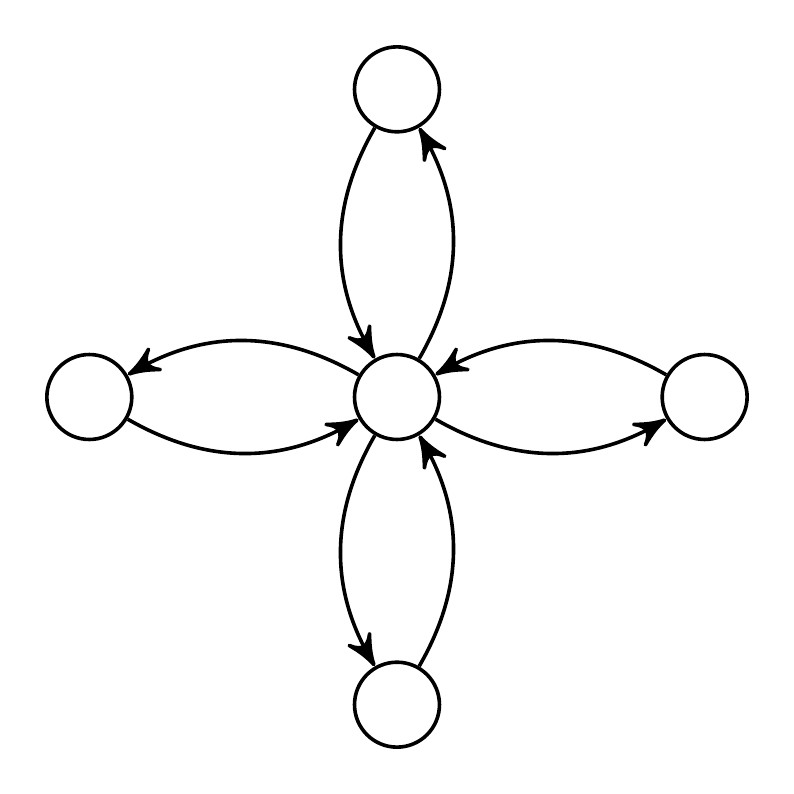
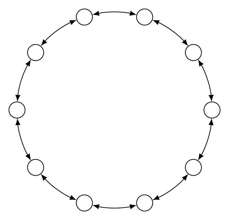
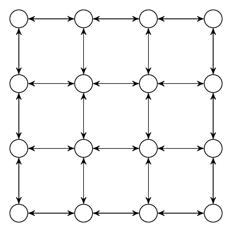
IV-D Star, Cycle and Grid Networks
We now examine the spectral gap impact for some interesting networks (Fig. 1), and derive explicit bounds for decentralization cost. As one of the famous examples in computer networks, we start with the star network. Regardless of the network size, existence of one central agent always preserves the network diameter, and therefore, we expect a benign scaling with network size. On the other side of the spectrum lies the cycle network where the diameter grows linearly with the network size. We should, hence, observe how the poor communication in cycle network affects the learning rate. Finally, as a possible model for sensor networks, we study the grid network where the network size scales quadratically with the diameter.
 |
 |
 |
Corollary 8
Proof:
The spectrum of the Laplacian of star and cycle graphs are well-known [27]. We have the eigenvalue set corresponding to communication matrix of star and cycle graphs as
respectively. Therefore, the proof of (a) and (b) follows immediately. The grid graph is the Cartesian product of two rings of size (due to wraparounds at the edges), and hence, its eigenvalues are derived by summing the eigenvalues of two -rings[27]. Therefore, the eigenvalue set takes the form
and the proof of (c) is completed. ∎
Let us use the notation to hide the poly log factors. Then, the bounds derived in Corollary 8 indicate that the algorithm requires iterations to achieve a near optimal log-distance from the true state in the star network. However, the rate deteriorates to respectively, in the cycle (respectively, grid) network. In all cases, the rate is proportional to the diameter of the network which is a natural indicator of information dissemination quality.
V Numerical Experiment : Binary Signal Detection
We now discuss distributed detection of signals transmitted through noisy channels. We first particularize the model to binary signals, and then present our simulation results in that context.
V-A Signal Detection in Communication Channels
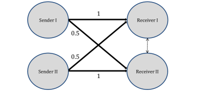
In information theory, data transmission can be modeled via a sender, a receiver and a channel. The channel is used to convey information from one end to another. In general, a faulty communication is possible, and it might be caused by channel noises, and imperfect modulation or demodulation (see e.g. [28, 29]). In what follows, we exemplify this point, and employ distributed detection to resolve it.
Suppose a 2-digit binary number is to be transmitted over a communication channel as depicted in Fig. 2. Sender I and sender II broadcast copies of the first and second digit, respectively. Receiver I (agent I) can recognize the first digit accurately555 To have the assumption A1 satisfied, we can think of accurate transmission as probability of success for some small . while the second digit is distorted with probability 1/2. On the other hand, receiver II (agent II) collects the exact value of the second digit at the terminal, and observes a misrepresented first digit with probability 1/2. In this example, the state space is , and let the true state be . We can see that none of the receivers can solely establish a reliable communication with senders as each of them has difficulty inferring one digit. More formally, it is straightforward to calculate that
which simply means and . However, the global identifiability of the true state holds as we have . Therefore, according to Lemma 3, exchanging information with each other, receivers are able to decipher the message transmitted by senders.
V-B Convergence of Beliefs
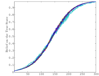
For purpose of simulation, we generate a strongly connected network of agents with a default communication matrix . Assume that there exist states in the world and agents are to discover the true state . At time , a signal is generated based on the true state such that . In other words, for agent , we have and is observationally equivalent to the true state. Therefore, each agent fails to distinguish from once relying on the private signals. However, since we have , the true state is globally identifiable. Consequently, in view of Lemma 3, we expect that all agents reach a consensus on the true state (Fig. 3), and learn the truth exponentially fast.
V-C Optimizing the Spectral Gap
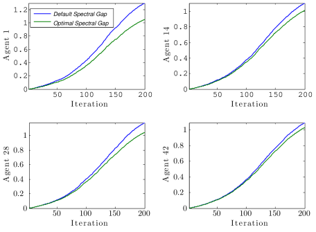
We now turn to optimizing the spectral gap to speed up learning. We proved in Proposition 6 that every default communication matrix can be adjusted to a matrix which has the optimal spectral gap when centralities are fixed. Setting the parameter in (10) equal to derived in Proposition 6, we obtain the optimal network. The dependence of decentralization cost to the spectral gap was theoretically proved in Theorem 5. Applying the results of Proposition 6 verifies that in the optimal network, agents suffer a lower decentralization cost comparing to the default network (Fig. 4).
V-D Sensitivity to Link Failure
Let us symmetrize the network in the previous section such that . In this case every agent is equally central, and we have . To study the impact of link failure, we sequentially select a random pair of agents in the network, and remove their connection. Each time that a link is discarded, we compute the decentralization cost in the new network at iteration , and continue the process until 50 bi-directional edges are eliminated from the network. In view of Proposition 7, we expect a monotone decrease in the spectral gap which amounts to a larger decentralization cost. We plot the cost for four agents in the network, and observe that the behavior is almost (not quite) monotonic (Fig. 5). The monotone dependence of the upper bound to the spectral gap (Theorem 5) does not necessarily guarantee a monotone relationship between cost and the spectral gap. Therefore, we can only roughly expect such behavior.
VI Conclusion
We considered a distributed detection model where a network of agents aim to learn the underlying state of the world. The private signals do not provide enough information for agents about the true state. Hence, agents engage in a local communication to compensate for their imperfect knowledge. Each agent iteratively forms a belief about the state space using the collected data in its neighborhood. We analyzed the learning procedure for a finite time horizon. To study the efficiency of our algorithm versus its centralized counterpart, we brought forward the idea of KL cost. It turned out that network size, spectral gap, centrality of each agent and relative entropy of agents’ signal structures are the key parameters that affect distributed detection. We established that allocating more informative signals to central agents as well as optimizing the spectral gap can speed up learning. We also proved that the learning rate deteriorates in the case of link failures, which can be seen as a side effect of poor communication. Finally, we would like to address a few issues in future works. In this paper, we discussed a communication model in which agents exchange information at every round. In some networks, all-time communication is potentially costly or unnecessary. Alternatively, agents can only contact each other when their signals are not informative enough about the true state. As another direction, we can consider scenarios where the signal distributions are not stationary. This generalizes the model to dynamic parameters where we can investigate detection robustness in changing environments.
Appendix : Proofs
Proof of Lemma 1. The proof is elementary, and it is only given to keep the paper self-contained. We write the Lagrangian associated to the update (3) as,
where we left the positivity constraint implicit. Differentiating above with respect to and , and setting the derivatives equal to zero, we get
respectively, for any . Combining the equations above and noting that is uniform, we have
which allows us to solve for and calculate the optimal solution as follows,
The proof for follows precisely in the same fashion. To calculate , notice that in view of the first update in (5) we have
where denotes the Kronecker product. The equation above represents a discrete-time linear system. Given the fact that for all and , the closed-form solution of the system takes the form
Therefore, extracting for each from the preceding relation completes the proof.
Proof of Lemma 2. Since the network is strongly connected and the corresponding is irreducible and aperiodic, by standard properties of stochastic matrices (see e.g. [21]), the diagonalizable matrix satisfies
| (14) |
for any , where is the stationary distribution of a Markov chain with transition kernel . Let us observe the following inequality
and recall that the identity always holds since any power of is stochastic. With that in mind, we use (14) to break the following sum into two parts to get
for any . Noting that , we have
Lemma 9
(McDiarmid’s Inequality) Let be independent random variables and consider the mapping . If for , and every sample , the function satisfies
then for all ,
Proof of Lemma 3. According to Lemma 1, we have
| (15) |
where we used the fact that for any . Since we know
we can simplify (15) as follows
| (16) |
For any , define
and note that is a function of random variables. As required in McDiarmid’s inequality in Lemma 9, set , fix the samples for random variables, and draw two different samples and for some and some . The fixed samples are simply cancelled in the subtraction, and we have
where we used assumption A1. Since any power of is stochastic, summing over and , we get
We now apply McDiarmid’s inequality in Lemma 9 to obtain
for . Setting the probability above to and taking a union bound over all states, we have for any
| (17) |
On the other hand, in view of assumption A1, we have
where we applied Lemma 2 to derive the last step. Using (4), we simplify above to get
| (18) |
for any . Plugging (18) into (17) and combining with (16), we have
with probability at least , and thereby completing the proof.
Proof of Lemma 4. We recall from the statement of the lemma that , and calculate the ratio for any as follows,
This entails
where we used Jensen’s inequality on the convex function . Setting the expectation measures in the right hand side of above to , and recalling the ratio from above, we conclude that,
| (19) |
where we applied Cauchy-Schwarz inequality in the last line. Then, we appeal to Jensen’s inequality again to get
Note that the function is nondecreasing over reals, and let in . The condition immediately implies that , so recalling that is the argument of exponential in above, we bound the right hand side as,
Plugging the bound above into (19), results in
Summing above over and recalling (6), concludes the proof.
References
- [1] R. R. Tenney and N. R. Sandell Jr, “Detection with distributed sensors,” IEEE Transactions on Aerospace Electronic Systems, vol. 17, pp. 501–510, 1981.
- [2] J. N. Tsitsiklis et al., “Decentralized detection,” Advances in Statistical Signal Processing, vol. 2, no. 2, pp. 297–344, 1993.
- [3] V. Borkar and P. P. Varaiya, “Asymptotic agreement in distributed estimation,” IEEE Transactions on Automatic Control, vol. 27, no. 3, pp. 650–655, 1982.
- [4] S. Kar, J. M. Moura, and K. Ramanan, “Distributed parameter estimation in sensor networks: Nonlinear observation models and imperfect communication,” IEEE Transactions on Information Theory, vol. 58, no. 6, pp. 3575–3605, 2012.
- [5] O. Dekel, R. Gilad-Bachrach, O. Shamir, and L. Xiao, “Optimal distributed online prediction using mini-batches,” The Journal of Machine Learning Research, vol. 13, no. 1, pp. 165–202, 2012.
- [6] A. Nedic and A. Ozdaglar, “Distributed subgradient methods for multi-agent optimization,” IEEE Transactions on Automatic Control, vol. 54, no. 1, pp. 48–61, 2009.
- [7] A. Nedic, A. Olshevsky, A. Ozdaglar, and J. N. Tsitsiklis, “On distributed averaging algorithms and quantization effects,” IEEE Transactions on Automatic Control, vol. 54, no. 11, pp. 2506–2517, 2009.
- [8] J.-F. Chamberland and V. V. Veeravalli, “Decentralized detection in sensor networks,” IEEE Transactions on Signal Processing, vol. 51, no. 2, pp. 407–416, 2003.
- [9] F. Bullo, J. Cortés, and S. Martinez, Distributed control of robotic networks: a mathematical approach to motion coordination algorithms. Princeton University Press, 2009.
- [10] N. A. Atanasov, J. Le Ny, and G. J. Pappas, “Distributed algorithms for stochastic source seeking with mobile robot networks,” Journal of Dynamic Systems, Measurement, and Control, 2014.
- [11] S. Shahrampour, S. Rakhlin, and A. Jadbabaie, “Online learning of dynamic parameters in social networks,” in Advances in Neural Information Processing Systems, 2013.
- [12] J. N. Tsitsiklis, “Problems in decentralized decision making and computation.” DTIC Document, Tech. Rep., 1984.
- [13] A. Jadbabaie, J. Lin, and A. S. Morse, “Coordination of groups of mobile autonomous agents using nearest neighbor rules,” IEEE Transactions on Automatic Control, vol. 48, no. 6, pp. 988–1001, 2003.
- [14] R. Olfati-Saber and R. M. Murray, “Consensus problems in networks of agents with switching topology and time-delays,” IEEE Transactions on Automatic Control, vol. 49, no. 9, pp. 1520–1533, 2004.
- [15] A. Jadbabaie, P. Molavi, A. Sandroni, and A. Tahbaz-Salehi, “Non-bayesian social learning,” Games and Economic Behavior, vol. 76, no. 1, pp. 210–225, 2012.
- [16] S. Shahrampour and A. Jadbabaie, “Exponentially fast parameter estimation in networks using distributed dual averaging,” in IEEE Conference on Decision and Control (CDC), 2013, pp. 6196–6201.
- [17] A. Lalitha, A. Sarwate, and T. Javidi, “Social learning and distributed hypothesis testing,” in International Symposium on Information Theory (ISIT), 2014, pp. 551–555.
- [18] K. Rahnama Rad and A. Tahbaz-Salehi, “Distributed parameter estimation in networks,” in IEEE Conference on Decision and Control (CDC), 2010, pp. 5050–5055.
- [19] J. C. Duchi, A. Agarwal, and M. J. Wainwright, “Dual averaging for distributed optimization: convergence analysis and network scaling,” IEEE Transactions on Automatic Control, vol. 57, no. 3, pp. 592–606, 2012.
- [20] A. Jadbabaie, P. Molavi, and A. Tahbaz-Salehi, “Information heterogeneity and the speed of learning in social networks,” Columbia Business School Research Paper, no. 13-28, 2013.
- [21] J. S. Rosenthal, “Convergence rates for markov chains,” Siam Review, vol. 37, no. 3, pp. 387–405, 1995.
- [22] J. D. Abernethy, E. Hazan, and A. Rakhlin, “Interior-point methods for full-information and bandit online learning,” IEEE Transactions on Information Theory, vol. 58, no. 7, pp. 4164–4175, 2012.
- [23] A. Nemirovskii and D. Yudin, Problem complexity and method efficiency in optimization. Wiley (Chichester and New York), 1983.
- [24] N. Cesa-Bianchi, G. Lugosi et al., Prediction, learning, and games. Cambridge University Press Cambridge, 2006, vol. 1.
- [25] A. Rakhlin and K. Sridharan, “Online learning with predictable sequences,” in Conference on Learning Theory, 2013, pp. 993–1019.
- [26] D. A. Levin, Y. Peres, and E. L. Wilmer, Markov chains and mixing times. American Mathematical Soc., 2009.
- [27] F. R. Chung, Spectral graph theory. American Mathematical Soc., 1997, vol. 92.
- [28] T. M. Cover and J. A. Thomas, Elements of information theory. John Wiley & Sons, 2012.
- [29] H. V. Poor, An introduction to signal detection and estimation. Springer, 1994.
- [30] C. McDiarmid, “Concentration,” in Probabilistic methods for algorithmic discrete mathematics. Springer, 1998, pp. 195–248.