The 2014 March 29 X-flare: sub-arcsecond resolution observations of Fe XXI $\lambda$1354.1

Abstract

The Interface Region Imaging Spectrometer (IRIS) is the first solar instrument to observe $\sim 10$ MK plasma at subarcsecond spatial resolution through imaging spectroscopy of the Fe xxi $\lambda$1354.1 forbidden line. IRIS observations of the X1 class flare that occurred on 2014 March 29 at 17:48 UT reveal Fe xxi emission from both the flare ribbons and the post-flare loop arcade. Fe xxi appears at all of the chromospheric ribbon sites, although typically with a delay of one raster (75 seconds) and sometimes offset by up to 1${{}^{\prime}}{{}^{\prime}}$. 100–200 km s^-1 blue-shifts are found at the brightest ribbons, suggesting hot plasma upflow into the corona. The Fe xxi ribbon emission is compact with a spatial extent of $<2$${{}^{\prime}}{{}^{\prime}}$, and can extend beyond the chromospheric ribbon locations. Examples are found of both decreasing and increasing blue-shift in the direction away from the ribbon locations, and blue-shifts were present for at least 6 minutes after the flare peak. The post-flare loop arcade, seen in Atmospheric Imaging Assembly (AIA) 131 Å filtergram images that are dominated by Fe xxi, exhibited bright loop-tops with an asymmetric intensity distribution. The sizes of the loop-tops are resolved by IRIS at $\geq 1$${{}^{\prime}}{{}^{\prime}}$, and line widths in the loop-tops are not broader than in the loop-legs suggesting the loop-tops are not sites of enhanced turbulence. Line-of-sight speeds in the loop arcade are typically $<10$ km s^-1, and mean non-thermal motions fall from 43 km s^-1 at the flare peak to 26 km s^-1 six minutes later. If the average velocity in the loop arcade is assumed to be at rest, then it implies a new reference wavelength for the Fe xxi line of $1354.106\pm 0.023$ Å.

1 Introduction

The ${}^{3}P_{0}$–${}^{3}P_{1}$ ground transition of Fe xxi gives rise to an emission line at 1354.1 Å that was first identified from Skylab S082B spectra by Doschek et al. (1975). It is the strongest emission line formed at temperatures $\geq 10$ MK that is found longward of the hydrogen Lyman limit, and it is of great interest for studying plasma dynamics during flares on account of the much higher spectral resolution possible at ultraviolet wavelengths compared to X-ray wavelengths. The first observations of Doschek et al. (1975) demonstrated for one flare that the line width decreased as the flare evolved, and Doppler motions did not exceed 20 km s^-1. Cheng et al. (1979) studied 17 Skylab flares and used $\lambda$1354.1 to determine non-thermal velocities ranging between 0 and 60 km s^-1. Note that the S082B instrument had a 2${{}^{\prime}}{{}^{\prime}}$ $\times$ 60${{}^{\prime}}{{}^{\prime}}$ slit but no spatial resolution along the slit, thus the spatial resolution of the instrument depended on the spatial extent of the observed flare.

Mason et al. (1986) analyzed seven flares observed with the Ultraviolet Spectrometer and Polarimeter (UVSP) on board the Solar Maximum Mission (SMM), and found examples of asymmetries in the line profile during the rise phase of flares that indicated plasma upflowing at speeds of up to 200 km s^-1. Smaller asymmetries were also found during the soft X-ray peaks of the flares, suggesting evaporation was continuing at this stage of the flare. The spatial resolution of UVSP was determined by the size of the entrance slit used, which could be as small as 3${{}^{\prime}}{{}^{\prime}}$ $\times$ 3${{}^{\prime}}{{}^{\prime}}$.

The Solar Ultraviolet Measurement of Emitted Radiation (SUMER) instrument on board the Solar and Heliospheric Observatory (SOHO) observed the Fe xxi line, but only in off-limb flares. A M7.6 flare on 1999 May 9 was captured with a full spectrum scan by SUMER and studied by Feldman et al. (2000), Innes et al. (2001) and Landi et al. (2003). The Fe xxi line was observed about 3 hours after the flare peak, and Feldman et al. (2000) derived a new rest wavelength of $1354.064\pm 0.020$ Å for the line, and Landi et al. (2003) found non-thermal broadening corresponding to 30–40 km s^-1. Fe xxi $\lambda$1354.1 was also recorded in the X-class flare of 2002 April 21, which produced a supra-arcade of hot plasma that displayed dynamic, dark voids (Innes et al., 2003a, b). Blueshifts of up to 1000 km s^-1 were seen in this data-set, and $\lambda$1354.1 was used to constrain the temperature of the dark voids. A further use of $\lambda$1354.1 from SUMER data was to study Doppler shift oscillations in hot active region loops (Kliem et al., 2002; Wang et al., 2003a), which are triggered by microflares and are interpreted as standing slow-mode magnetoacoustic waves (Wang et al., 2003b).

The Fe xxi line was first reported in a non-solar spectrum by Maran et al. (1994) who measured it in a Goddard High Resolution Spectrometer spectrum of the star AU Microscopii. A survey of measurements of the line in cool stars was presented by Ayres et al. (2003) based on Space Telescope Imaging Spectrograph (STIS) data.

Fe xxi is only expected to be found in the solar spectrum during flares and there are two key spatial locations expected from the standard model of solar flares. The standard model (see the review of Benz, 2008) specifies an energy release site in the corona, usually assumed to be the location of magnetic reconnection. Energy from the release site is transmitted down the legs of coronal loops in the form of non-thermal particles, a thermal conduction front, or Alfvén waves. The energy is deposited in the dense chromosphere, leading to plasma heating, and the subsequent expansion of the plasma results in the “evaporation” of hot plasma into the coronal loops. Fe xxi is formed at $\approx 10$ MK, and we expect to find 10 MK plasma concentrated at the loop footpoints due to the initial chromospheric heating, followed later by the appearance of bright 10 MK loops that are formed from the evaporated plasma. A key prediction of the standard flare model is that the plasma at the footpoints will flow upwards into the loops as the evaporation process proceeds and thus blue-shifted emission lines are expected. Spatially-resolved spectral data from the Coronal Diagnostic Spectrometer (CDS) on board SOHO, and the EUV Imaging Spectrometer (EIS) on board the Hinode spacecraft have demonstrated that blue-shifted emission is seen in emission lines of Fe xix, Fe xxiii and Fe xxiv and speeds can be as high as 400 km s^-1 (Teriaca et al., 2003, 2006; Milligan et al., 2006; Del Zanna et al., 2006; Watanabe et al., 2011; Young et al., 2013). The flare loop footpoints are expected to coincide with the flare ribbons that are seen in H$\alpha$ and UV continuum images, although this can not be directly confirmed with CDS and EIS, which observe extreme ultraviolet radiation.

The Interface Region Imaging Spectrometer (IRIS) was launched in 2013 June and it observes the 1332–1358 Å wavelength region at a spatial resolution of 0.33–0.40${{}^{\prime}}{{}^{\prime}}$, significantly better than the previous instruments that have observed the Fe xxi line. The high spatial resolution enables the fine-scale structure of the Fe xxi line to be investigated, particularly with regard flare loops and their footpoints. The first study of the Fe xxi line using IRIS data was performed by Tian et al. (2014) who analyzed the C1.6 class flare that peaked at 17:19 UT on 2014 April 19. The authors reported a red-shifted component that could be attributed to the downward reconnection outflow expected from the standard solar flare model. In this paper we present observations obtained by IRIS of the X1 class flare that occurred on 2014 March 29, peaking at 17:48 UT (SOL2014-03-29T17:48). Judge et al. (2014) investigated photospheric heating and the causes of the sunquake associated with this flare using data from the Facility Infrared Spectrometer at the Dunn Solar Telescope. The Balmer continuum increase associated with the flare was presented by Heinzel & Kleint (2014) who used the near-UV continuum increase measured by IRIS around 2800 Å. The filament eruption associated with the flare was studied by Kleint et al. (2014, ApJ, in press), who combined multiple data-sets, including from IRIS, to measure the rapid acceleration of the filament, which reached speeds of up to 600 km s^-1. Li et al. (2014, ApJ, in press) combined data from IRIS and EIS to study evaporation flows at specific sites in the active region. They demonstrated that the high-temperature evaporation flows move with time in response to the flare ribbon separation, and find redshifts of transition region lines at the locations of the blue-shifted hot lines (10 MK). The present work differs from this latter work in studying all of the IRIS ribbons sites, and investigating the connection to the chromospheric flare ribbons. In addition we also study the Fe xxi emission from the post-flare loop arcade.

The paper is structured as follows. Sect. 2 gives an overview of the March 29 flare observation and describes the data-sets. Sect. 3 defines flares ribbons and kernels in the context of the IRIS data, and Sect. 4 describes how the Fe xxi emission in the vicinity of the ribbons behaves. Sect. 5 discusses properties of the post-flare loop arcade, and Sect. 6 summarizes the results.

2 Observations

The flare occurred in active region AR 12017 which was part of a larger complex that included AR 12018. The 1–8 Å GOES light curve is plotted in Figure 1 and shows that the flare began at 17:35 UT with an initial rise from a GOES class level B9 to C3 by 17:41 UT. A rapid rise to the X1 level began at 17:44 UT, with the peak reached at 17:48 UT.

Figure 1: The GOES 1–8 Å light curve for the period 17:30–18:05 UT on 2014 March 29. Short vertical lines indicate the start and end times of the IRIS rasters, and the IRIS raster numbers are indicated.

IRIS is described in detail by De Pontieu et al. (2014) and is briefly summarized here. The instrument returns narrow-slit spectral data over three wavelength bands of 1332–1358, 1389–1406 and 2782–2834 Å, and a slit-jaw imager can produce images centered at 1330, 1400, 2796 and 2832 Å, giving context images for the spectra. The spectrometer slit is 0.33${{}^{\prime}}{{}^{\prime}}$ wide, and the detector pixel sizes correspond to 0.167${{}^{\prime}}{{}^{\prime}}$. The strongest emission lines observed by the instrument are Mg ii $\lambda$$\lambda$2796.4, 2803.5, C ii $\lambda$$\lambda$1334.5, 1335.7, and Si iv $\lambda$$\lambda$1393.8, 1402.8, which are formed in the chromosphere and transition region. Fe xxi $\lambda$1354.1 is the only coronal line in the present data-set that can yield sufficient signal-to-noise for detailed studies of line profiles.

For the present flare observation IRIS performed 180 raster scans over the period 14:09 to 17:54 UT. Each scan consisted of eight slit positions separated by 2${{}^{\prime}}{{}^{\prime}}$, giving a total raster size of 14.33${{}^{\prime}}{{}^{\prime}}$. The field-of-view in the solar-Y direction was 175${{}^{\prime}}{{}^{\prime}}$ and 8 second exposures were used. The duration of each raster was 75 seconds. A slit-jaw image was obtained with each raster exposure: images at 2796 Å were obtained for exposures 1, 3, 5 and 7; images at 1400 Å were obtained for exposures 0, 4 and 6; and an image at 2832 Å was obtained for exposure 2. Saturation on the detector was a problem for the strong IRIS lines during the flare (particularly Si iv $\lambda$1402), but Fe xxi $\lambda$1354.1 was not saturated at any location. We focus on rasters 171–179, which cover the rise and initial-decay phases of the flare (Figure 1). We note that there was weak Fe xxi from the active region prior to this time period that is related to the weaker C3 event, but our focus in the present work is on the flare ribbons and post-flare loops of the X1 event. As a shorthand in the present work we will refer to specific IRIS exposures as, e.g., R174E0, which refers to raster no. 174 and exposure no. 0. The raster numbers go from 0 to 179 and the exposure numbers from 0 to 7 (note that IRIS rasters from east to west). When giving times for these exposures, we give the mid-time of the exposure.

Level-2 IRIS data were downloaded from the IRIS website and they are corrected for most instrumental effects, including geometric distortions, flat-fields and spatial alignments. The version of the calibration processing routine (IRIS_PREP) applied to the data was 1.27. Intensities are given in data-number (DN) units and 1-$\sigma$ uncertainties are derived as follows. For the FUV channel, one DN corresponds to four detected photons (De Pontieu et al., 2014), so $d$ DN yield $p=4d$ photons. Assuming Poisson noise, the uncertainty on $p$ is $\sqrt{p}$, however the dark current uncertainty, $\sigma_{\rm dc}$, also needs to be included, giving

$$\sigma_{p}=\sqrt{4d+(4\sigma_{\rm dc})^{2}}$$ (1)

De Pontieu et al. (2014) give a value of $\sigma_{\rm dc}=3.1$ DN for the FUV channel. Defining the fractional error to be $f=\sigma_{p}/p$, the uncertainty on $d$ is then $\sigma_{d}=fd$. This method for computing the intensity uncertainties is implemented in the Solarsoft IDL routine IRIS_GETWINDATA.

We found that the best way to study the $\lambda$1354.1 emission line for this data-set was through exposure images (wavelength vs. solar-Y) as they allow the difference in morphology between the broad $\lambda$1354.1 line and the narrow blending cool lines to be more easily discerned. The raster is too sparse for X-Y images to accurately reflect the intensity distribution across the raster and for this it is better to consider 131 Å images from the Atmospheric Imaging Assembly on board the Solar Dynamics Observatory.

The AIA instrument is described in Lemen et al. (2012), and the images considered in the present work are from the 131 Å filter (hereafter referred to as “A131”), which is dominated by Fe xxi $\lambda$128.75 during flares (O’Dwyer et al., 2010) and thus is ideal for comparisons with the IRIS slit images. Additional contributing lines are Fe xx $\lambda$132.84 and Fe xxiii $\lambda$132.91. The image spatial scale is 0.6${{}^{\prime}}{{}^{\prime}}$ per pixel, and the cadence is 12 seconds. An automatic observing procedure is initiated during flares when count rates become large. Every alternate frame remains at the nominal exposure time, with the exposure times for the remaining frames adjusted through an automatic exposure control mechanism. Despite this, the rapid intensity increases during the flare still led to many frames that were badly affected by saturation. In the present case from 17:46 UT to the end of the IRIS sequence at 17:54:19 UT there are only 12 A131 exposures for which saturation is sufficiently low to allow comparison with the IRIS data, however these images still yield valuable comparisons with the IRIS data as demonstrated in the following sections.

The wavelength of Fe xxi $\lambda$1354.1 was given as $1354.08\pm 0.05$ Å by Sandlin et al. (1977) based on Skylab S082B measurements, and Feldman et al. (2000) gave a value of $1354.064\pm 0.020$ Å from SUMER spectra. In the present article we derive a new value for the reference wavelength of $1354.106\pm 0.023$ Å (Appendix B). The temperature of maximum emission of $\lambda$1354.1 is $\log\,T/{\rm K}=7.06$, as obtained from atomic data in version 7.1 of the CHIANTI database (Dere et al., 1997; Landi et al., 2013). This temperature translates to a full-width at half-maximum (FWHM) emission line width of 0.438 Å, or 96.9 km s^-1 in velocity space. The instrumental width is 25.85 mÅ (De Pontieu et al., 2014) and so is essentially negligible when studying $\lambda$1354.1 line width measurements.

3 Flare ribbons

As stated in the Introduction, energy from the coronal energy release site of a flare travels to the chromosphere down coronal loop legs, leading to heating that is revealed through bright flare ribbons seen in H$\alpha$ and UV continuum images. We expect to see Fe xxi emission at these ribbons due to the rapid heating that occurs there. In this section we discuss properties of flare ribbons and their appearance in IRIS data.

Flare ribbons are a characteristic feature of H$\alpha$ flare observations and they appear as narrow, curved, bright lines across the solar surface. Pairs of ribbons are common, but they can have complex shapes and discontinuities. The ribbons resolve into lines of compact kernels, and the sizes of the kernels have been measured to 0.6–1.9${{}^{\prime}}{{}^{\prime}}$ in one case, with smaller sizes corresponding to deeper atmospheric depths (Xu et al., 2012). Flare kernels can be seen in white light flares, but are much more easily seen in the UV continuum, such as the 1700 Å channel of the Transition and Coronal Explorer (TRACE, Handy et al., 1999) and AIA. Young et al. (2013) reported an AIA measurement of a flare kernel and found that it emitted in all of the the EUV channels of AIA, with a size at the resolution of the instrument ($\approx 1.2$${{}^{\prime}}{{}^{\prime}}$).

The IRIS instrument observes at FUV and near-ultraviolet (NUV) wavelengths, and the ribbons can be measured in both the continuum and the emission lines. The FUV continuum enhancement during flares is believed to be driven by backwarming from C ii $\lambda$$\lambda$1334, 1335 and Si iv $\lambda$$\lambda$1393, 1402 (Doyle & Phillips, 1992). We thus expect the FUV continuum ribbons to be correlated with the brightness of these emission lines (which are measured by IRIS). Although beyond the scope of the present work, we note that inspection of the March 29 flare suggests that this is indeed the case.

The development of the March 29 ribbons is best studied with the IRIS slit-jaw data, in particular the 2796 Å images that were obtained at an 18 second cadence. These images show significantly less saturation than the 1400 Å images, allowing the ribbon evolution to be seen more clearly. The 2796 Å images are dominated by emission from Mg ii and we note that the ribbon structures are less well-defined than in the 1400 Å images, although this may just reflect the lower spatial resolution of the longer wavelength channel (De Pontieu et al., 2014). Movie 1 shows the development of the ribbons over the period 17:42:05 to 17:49:15 UT, and Figure 2 shows images from this movie at 17:45:12 and 17:46:08 UT. The initial impression from the movie is that there are two ribbons: a north ribbon (N1) between X=505 and 515, and a south ribbon (S1) that extends across the full X-range of the images in Figure 2. The north ribbon at 17:45:12 UT is seen to double back on itself, with the two arms being separated by only 2–4${{}^{\prime}}{{}^{\prime}}$. The arms move towards each other slightly before the northerly arm fades, leaving the southerly arm with a distinctive hook on the east side at around X=495 (Figure 2b). In addition to this ribbon, there is a small ribbon that is labeled N2 in Figure 2b and is bright in exposures E6 and E7 of the rasters. There is a faint, eastward extension of this ribbon that possibly connects to N1.

The south ribbon becomes much brighter than the north ribbon, with some saturation in the 2796 Å images. It also moves southwards by about 10${{}^{\prime}}{{}^{\prime}}$ from 17:45:12 UT to the end of the movie at 17:49:15 UT. Between X=510 and 525, the southward movement of the ribbon leaves behind a patch of enhanced emission and the IRIS spectra demonstrate that the FUV continuum is enhanced in this region. The spectra also reveal that the initial position of the south ribbon (marked with S1 in Figure 2a) maintains enhanced continuum and emission lines even as the main ribbon (S2) advances southwards. From Movie 1 it is not clear if S2 actually represents the new position of S1 or whether it is a distinct ribbon. A crucial 1400 Å slit-jaw image at 17:45:26 UT that may resolve this question is too saturated to allow the south ribbon to be identified. We distinguish S1 from S2 based on the fact that it retains a distinctive signature in terms of enhanced continuum and emission lines.

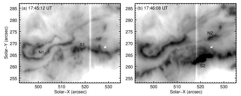
Figure 2: IRIS 2796 Å slit-jaw images at two different times during the development of the flare ribbons. An inverse logarithmic intensity scaling is used.

In the following section we are interested in the location of Fe xxi emission relative to the ribbons, and we define the ribbons in the spectral images as being the locations where the FUV continuum is enhanced. Comparison of 1400 Å and 2796 Å slit-jaw images, and FUV and NUV spectral images suggests that the FUV continuum ribbons directly correspond to the 2796 Å image ribbons shown in Movie 1.

4 Fe XXI at the ribbons

In this section we interpret the Fe xxi emission close to the flare ribbon sites in terms of the standard flare model, which invokes heating of the chromosphere at the footpoints of an arcade of coronal loops to explain the bright chromospheric flare ribbons. The plasma is heated to temperatures of $\sim 10$ MK, and it rises up the loops, filling them with hot, dense plasma to create the bright post-flare loop arcade. The loop footpoints will emit in Fe xxi $\lambda$1354.1 and we expect to see blue-shifts from the evaporating plasma. Key questions that will be addressed are: (i) does Fe xxi always appear at the chromospheric ribbon sites? (ii) is Fe xxi alway blue-shifted at the ribbons? (iii) is there a delay between the chromospheric ribbon appearing and Fe xxi being produced? and (iv) where the position of the ribbon moves in time (implying new sets of nested loops being progressively heated) do we continue to see blue-shifted Fe xxi emission at the older sites?

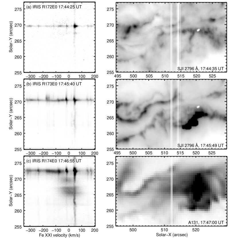
Figure 3: Sequence of three images showing the development of the Fe xxi $\lambda$1354.1 line at a location on the N1 flare ribbon. The left column shows IRIS detector images with a reverse–linear intensity scaling applied. A saturation has been applied to better reveal the weak Fe xxi line. The right columns of panels a and b show IRIS 2796 Å slit-jaw images, with the location of the IRIS slit corresponding to the left column images indicated by white parallel lines. An inverse–logarithmic intensity scaling has been applied. The right column of panel c shows an A131 image for which an inverse–square-root intensity scaling has been applied. The parallel white lines indicate the location of the IRIS slit.

Our first task is classify the spectroscopic observations of the four ribbons (N1, N2, S1 and S2), and Table 1 presents the results. By inspecting the sequence of rasters we identify the time at which the ribbon appears in each of the eight raster exposures. For example, the N1 ribbon is only observed in exposures E0 and E1, and it first appears in E0 during raster R172 (17:44:25 UT). This is illustrated in Figure 3 where panel a shows the FUV continuum and chromospheric lines brighten over a small spatial region of width only 0.3${{}^{\prime}}{{}^{\prime}}$ in the solar-Y direction. There is no Fe xxi emission in this exposure. The next raster, R173 (Figure 3b), shows that the continuum and chromospheric lines have brightened and now Fe xxi is present, slightly offset in Y from the continuum, although it is weak. Figure 4a shows a 1D spectrum obtained at Y=270.0${{}^{\prime}}{{}^{\prime}}$, offset 0.33${{}^{\prime}}{{}^{\prime}}$ from the ribbon to better show the Fe xxi line. It is clearly seen to be broad and blue-shifted by around 100 km s^-1. Figure 3b shows that the Fe xxi emission is very compact in the Y-direction (around 0.3${{}^{\prime}}{{}^{\prime}}$) and slightly offset from the location of the ribbon emission. The ribbon moved slightly northwards between rasters R172 and R173, and so the offset may indicate that Fe xxi is emitted from the earlier location of the ribbon. Figure 3c shows the next raster with a clearly visible Fe xxi line at the ribbon site, and two additional patches of Fe xxi emission at 266${{}^{\prime}}{{}^{\prime}}$ and 270${{}^{\prime}}{{}^{\prime}}$ that can be identified as loop emission due to their broader extent in the Y-direction and their small Doppler shifts. All three Fe xxi locations can be identified in the co-temporal A131 image, demonstrating that this image mostly displays Fe xxi at this stage of the flare.

Table 1: Properties of the IRIS flare ribbons.

			Ribbon	Fe xxi	Velocity
Ribbon	Exposure	Solar-Y	appears	appears	(km s-1)	Position	Morphology
N1	0	269.6	44:25 [172]	45:40 [173]	$-100$	Offset	Compact
	1	272.1	45:49 [173]	45:49 [173]	$-100$	Ribbon	Compact
N2	3	270.4	46:08 [173]	46:08 [173]	$0$	Ribbon	Extended (N)
	4	271.1	46:17 [173]	46:17 [173]	$+30$	Ribbon	Extended (N,S)
	5	271.2	46:27 [173]	46:27 [173]	$0$	Ribbon	Compact
	6	271.4	44:06 [171]	46:36 [173]	$-120$	Ribbon	Diagonal-in (S)
	7	271.3	45:31 [172]	46:45 [173]	$-10$	Ribbon	Extended (N,S)
S1	1	268.3	45:49 [173]	47:04 [174]	$0$	Ribbon	Extended (N,S)
	2	268.3	44:44 [172]	45:59 [173]	$-20$	Ribbon	Extended (S)
	3	267.9	44:53 [172]	46:08 [173]	$-30$	Offset	Extended (S)
	4	268.2	45:03 [172]	46:17 [173]	$-10$	Ribbon	Extended (S)
	5	267.2	45:12 [172]	46:27 [173]	$0$	Ribbon	Extended (S)
S2	1	262.2	45:49 [173]	47:04 [174]	$-100$	Ribbon	Diagonal-in (N)
	2	261.8	45:59 [173]	47:14 [174]	$-120$	Offset	Diagonal-in (N)
	3	262.5	46:08 [173]	47:23 [174]	$-220$	Ribbon	Diagonal-in (N)
	4	262.4	46:17 [173]	46:17 [173]	$-120$	Offset	Compact
	5	261.8	46:27 [173]	47:42 [174]	$-160$	Offset	Diagonal-out (N)
	6	266.1	45:21 [172]	45:21 [172]	$-20$	Offset	Diagonal-out (N)
	7	265.3	45:31 [172]	48:00 [174]	$-110$	Offset	Compact

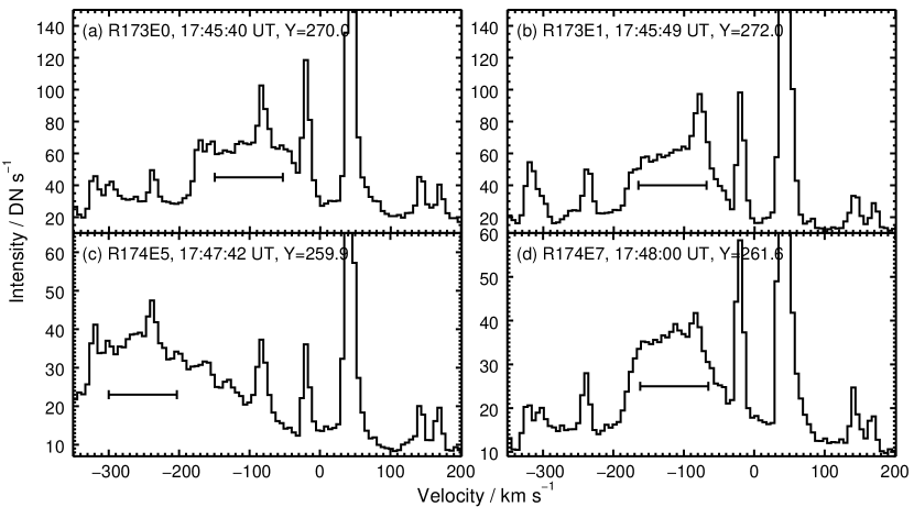
Figure 4: Four examples of Fe xxi $\lambda$1354.1 line profiles from locations at or close to the flare ribbons. The profiles have been obtained for individual solar-Y pixels, and the Y-values are indicated on the plots. The horizontal lines show the thermal width expected for $\log\,T=7.06$, the temperature of formation of Fe xxi.

We repeat this analysis for all of the other ribbon locations, giving the results in Table 1. In several locations interpretation is not easy, for example due to contamination by overlying Fe xxi loop emission which is identified by emission close to the rest wavelength of the line, and by a greater spatial extent in the solar-Y direction. There are also cases where there are two ribbons very close to each other that we interpret as a kink in the ribbon in which the slit crosses the ribbon twice. Examples include R173E5 and R172E7, and evidence for the kinked ribbons can be seen in Movie 1. We choose the brighter ribbon location in these cases.

Figures 3 and 4a demonstrate that a number of chromospheric lines become strong at the ribbon location, compromising studies of the Fe xxi line. The examples from the March 29 flare show that the blending lines are always present at the ribbons, although they are stronger for the S2 ribbon compared to the other ribbons. A further complication is that some of the lines, particularly, Si ii $\lambda$1352.64 and $\lambda$1353.72 (at velocities $-325$ and $-85$ km s^-1 relative to $\lambda$1354.1), can exhibit significant broadening and Doppler shifts in some locations. Further examples of ribbon spectra are shown in Figure 4, and a discussion of the blending lines is given in Appendix A.

The results for the 19 ribbon sites firstly confirm that all of the ribbon locations can be identified with co-spatial or slightly offset Fe xxi emission, although the emission line is not always blue-shifted. In general there is a lag of one raster (75 seconds) between the first appearance of the chromospheric ribbon and the first appearance of Fe xxi at, or close-to the ribbon site.

Ribbons N1 and S2 are the brightest ribbons and they fit the classical picture of two approximately parallel ribbons located either side of the polarity inversion line that separate as the flare progresses. Of the nine sites along these ribbons, eight of them show blue-shifted Fe xxi emission consistent with the chromospheric evaporation scenario. Ribbons N2 and S1 are different in that they are dimmer and show little or no motion with time (Movie 1). Only one location (R173E6) shows a large Fe xxi blueshift, even though the line can be clearly identified with the chromospheric site. The smaller blueshifts may indicate that gentle evaporation is occurring at these sites, although there is one location where a redshift is found (ribbon N2, exposure 4).

In Table 1 we list the position and morphology of the Fe xxi emission as seen on the detector images. The position can either be coincident with the chromospheric location, or offset from it. The offsets are small, $\leq 1$${{}^{\prime}}{{}^{\prime}}$, but significant at the IRIS spatial resolution. Note that the majority of offset Fe xxi emission is associated with the fast-moving S2 ribbon. The morphology of the Fe xxi emission is expressed according to the spatial extent in the Y-direction. Compact and extended indicate whether the emission extends less than or more than 1${{}^{\prime}}{{}^{\prime}}$, while “diagonal-in” and “diagonal-out” refer to extended emission that changes position in the wavelength direction with position. Examples are shown in Figure 5.

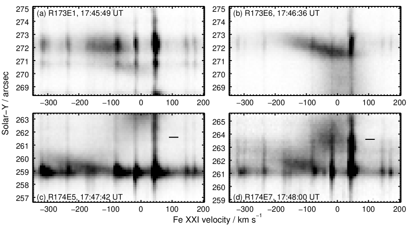
Figure 5: Four IRIS detector images showing different examples of Fe xxi emission at the flare ribbon sites. An inverse-linear intensity scaling has been applied, and the images have been saturated to better reveal the Fe xxi line. Short horizontal lines on panels c and d show the position of the flare ribbon in the previous rasters.

The interpretation of the extended, diagonal-in and diagonal-out emission types is not straightforward. For example, if the IRIS slit is aligned along the leg of one of the post-flare loops, then we may expect to see a large blue-shift of Fe xxi at the location of the flare ribbon, corresponding to evaporating chromospheric plasma. Further up the loop leg we may expect the magnitude of the blueshift to decrease as the velocity of the upflowing plasma decreases. This may explain the morphology of Fe xxi from the N2 ribbon for which the blueshift decreases from over 100 km s^-1  to 0 km s^-1 over less than 2${{}^{\prime}}{{}^{\prime}}$ (Figure 5b) – one of the diagonal-in types.

However, we know that the N1 and S2 ribbons change position with time, and so examples such as Figure 5c and d – diagonal-out and offset-extended types, respectively – may take their appearance because Fe xxi is emitted from an earlier location of the ribbon. In Figure 5c and d we have indicated the locations of the chromospheric ribbon in the previous rasters (obtained 75 seconds earlier) with a short horizontal line, demonstrating that the ribbon moved by around 2.5${{}^{\prime}}{{}^{\prime}}$ in each case. Figure 5c shows larger blueshifts about 0.5–1.0${{}^{\prime}}{{}^{\prime}}$ away from the ribbon site, so this may indicate that the blueshift at a fixed spatial location increases sometime after the initial burst of chromospheric heating that causes the chromospheric ribbon. Figure 5c does not show such a striking velocity pattern, but the brightest Fe xxi emission occurs about 0.5${{}^{\prime}}{{}^{\prime}}$ from the emission, and there is quite bright Fe xxi emission at the earlier location of the ribbon, although with a velocity only around $-20$ km s^-1. Close inspection of both the R174E5 and R174E7 locations does show that Fe xxi is present at all Y-locations between the previous and new ribbon locations, even though the brightness is variable.

What is clear from the fast-moving S2 ribbon is that the ribbon does not leave behind a trail of uniformly bright and blue-shifted Fe xxi at the former locations of the ribbon. Instead there is patchy emission that is usually brightest close to or at the current ribbon site, and that can have a range of velocities. This may reflect the non-uniform process that heats the chromosphere.

The IRIS observations terminate at 17:54:19 UT, only 6 minutes after the flare peak, and blue-shifted Fe xxi is still present at this time as demonstrated in Figure 6. This figure shows the LOS velocity of $\lambda$1354.1 and the FUV continuum level as determined from fits to the IRIS spectra in the 1352.3–1355.9 Å region – see Sect. 5. The S2 ribbon is still visible through an enhanced continuum level, and $\lambda$1354.1 is blue-shifted by 20–60 km s^-1  in exposures E4–7 at the location of the ribbon. There are also blueshifts related to the former position of the N1 ribbon seen in exposures E0–1, although there is no enhanced continuum at these locations.

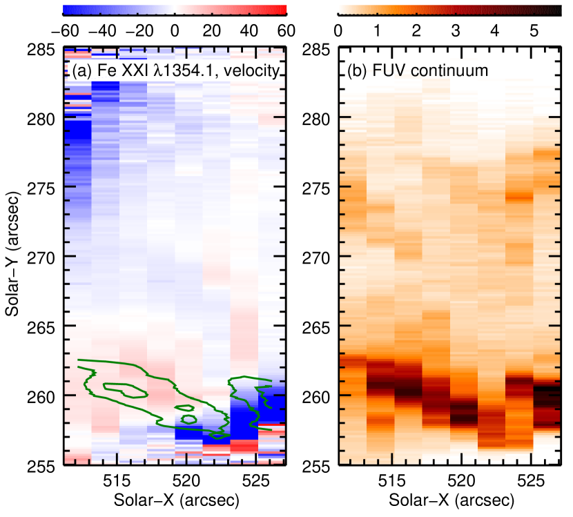
Figure 6: The left panel shows the LOS velocity of Fe xxi $\lambda$1354.1 from IRIS raster R179 (17:53:05–17:54:20 UT), as derived from a Gaussian fit. The right panel shows the FUV continuum level neighboring the Fe xxi line, and the green contours on panel a show the continuum level at 2.5 and 4.5 DN.

To summarize the results in relation to the four questions posed earlier in this section:

• Fe xxi is found at all of the chromospheric ribbon sites.

• Fe xxi is not always blue-shifted at the ribbon sites. However for the two brightest ribbons (N1, S2) the line is blue-shifted at 8 of the 9 sites. The N2 and S1 ribbons seem to be anomalous and generally do not show blueshifts.

• There is generally a lag of 75 seconds (the raster cadence time) before the line appears.

• The S2 ribbon moves quite rapidly over the solar surface, and Fe xxi is found at the previous locations of the ribbon. However, the emission is patchy and the magnitudes of the blueshifts vary.

In addition to these points, we note that the velocities of Fe xxi $\lambda$1354.1 at the ribbons are generally quite low, with values typically around $-100$ km s^-1 (column 6 of Table 1 and Figures 4a,b and d), significantly smaller than the velocities of $\approx-400$ km s^-1 found by Watanabe et al. (2011) and Young et al. (2013) from the Fe xxiii and Fe xxiv lines observed by EIS for two flares. This may be due to lower velocities at the cooler temperature of Fe xxi and a less favorable line-of-sight, although we also note that the IRIS data window used for the observation did not extend beyond $-350$ km s^-1 from the line center, thus very large velocities $\leq-400$ km s^-1 could not be detected. The largest blueshift seen in the IRIS data was from the S1 ribbon observed in R174E5 (Figure 5c) for which the centroid reached $\approx-250$ km s^-1 (Figure 4c). The profile was also very broad and apparently asymmetric. An asymmetric profile can also be identified from exposure R174E7 (Figure 4d). The blending lines complicate interpretation of the $\lambda$1354.1 line widths, but the profiles shown in Figure 4 have FWHMs at least as wide as the thermal width (96.9 km s^-1), and significantly larger in the case of Figure 4c.

Another contrasting feature with the profiles presented by Watanabe et al. (2011) and Young et al. (2013) is the lack of a two-component structure to the Fe xxi line, in particular the absence of a component near the rest wavelength. This may suggest that the EIS observations did not resolve the upflowing flare kernel sites from the stationary flare loop plasma, although Young et al. (2013) were able to demonstrate that the flare kernel they studied was isolated in co-temporal AIA images. Careful alignment of IRIS and EIS data is needed to determine whether the stationary component is missing from the Fe xxi line or whether it is simply due to a blending of loop and footpoint emission in the EIS data.

To summarize, Fe xxi $\lambda$1354.1 is not easy to measure at the flare ribbons on account of the intrinsically weak emission and the presence of a number of cool emission lines, some of which are broadened and/or demonstrate enhanced short wavelength wings at the ribbon site. However, the IRIS data show that Fe xxi is seen at or very close to all of the ribbon locations, typically about 75 seconds after the ribbons appear. Blueshifts typically correspond to velocities of $-100$ to $-200$ km s^-1, and the spatial extent (in solar-Y) of the Fe xxi ribbon emission is about 1${{}^{\prime}}{{}^{\prime}}$. A single emission line component is always seen at the ribbons and the widths are at least as large as the thermal width of the line. Blue-shifted Fe xxi emission at the ribbon locations is clearly seen until the end of the IRIS sequence at 17:54 UT, six minutes after the flare peak.

5 Fe XXI in the flare loops

Fe xxi emission from the post-flare loop arcade began to dominate at 17:47 UT and Figure 7 shows three A131 images obtained between 17:48 and 17:53 UT. A striking feature of these images, particularly at 17:53:00 UT, is that the loops had bright knots of emission towards the loop apexes. This feature of post-flare loops has been reported previously from Yohkoh X-Ray Telescope data (Acton et al., 1992; Feldman et al., 1994). An asymmetry in the intensity profile across the loop-tops is also striking, with the intensity dropping quite sharply on the north sides of the knots, but more smoothly on the south sides. This is illustrated in Figure 8 where the intensity profile along an arc chosen to align with a flare loop from the 17:50:36 UT exposure is plotted. The asymmetry in the intensity distribution is clearly seen, with the intensity falling to its half-maximum value within 1 Mm on the north side of the apex, and within 2.2 Mm on the south side. Intensities along the displayed arc were derived through bilinear interpolation of the original image. We note that the exposure time for the 17:50:36 UT is not correct in the AIA data file, and so the commanded exposure time is used instead. This introduces an uncertainty of $\pm 7$% in the stated intensities (P. Boerner, 2014, private communication). IRIS spectra allow the properties of the loop-top brightenings to be compared with the loop legs.

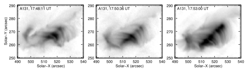
Figure 7: Three A131 images showing the post-flare loop arcade at different times. A cubed-root scaling has been applied and the color table reversed. The brightest areas (black) are saturated in each of the frames.

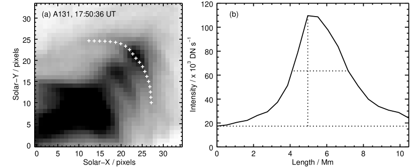
Figure 8: Panel (a) shows an A131 image from 17:50:36 UT. A square-root intensity scaling has been applied and the color table reversed. Interpolated intensities for the spatial locations identified by crosses on this image are plotted in Panel (b). Dotted lines show the locations of the maximum, minimum and half-maximum intensities.

Inspection of the $\lambda$1354.1 profiles in the post-flare loops shows that they are very close to Gaussian in shape except for the blend with C i $\lambda$1354.29, which is present in most spectra. For this reason we perform automatic Gaussian fits to the IRIS rasters, and extract intensity, velocity and line broadening parameters for the loop locations. At each spatial location we perform a three Gaussian fit to the wavelength window containing the Fe xxi line, with the additional two Gaussians used for C i $\lambda$1354.29 and O i $\lambda$1355.60. The EIS_AUTO_FIT suite of software (Young, 2013) developed for the Hinode/EIS mission was modified to perform the fitting. This software allows parameter limits to be applied to the Gaussians to prevent spurious fits. For example, Fe xxi $\lambda$1354.1 was restricted to full-width at half-maximum (FWHM) values between 0.35 and 1.41, while the much narrower O i $\lambda$1355.60 line was restricted to FWHM values between 0.023 and 0.14 Å.

From the Gaussian fits we can compare how parameters in the bright loop-tops compare with the loop legs. In Figure 9 we show an example from R179E6 (17:54:06 UT). This demonstrates that the LOS velocity is approximately zero at the loop-top (Y=271–274${{}^{\prime}}{{}^{\prime}}$), but increases to 7–8 km s^-1 in the southern loop legs (Y=263–266${{}^{\prime}}{{}^{\prime}}$), suggesting a draining of plasma to the loop footpoints. The line width shows no clear distinction between the loop-top and the legs, showing that the loop-top is not hotter than the legs, nor does it have an additional broadening component that may indicate turbulence. We note that Jakimiec et al. (1998) suggested a model for bright loop-tops whereby there are tangled magnetic field lines at the loop-top, and the motion of plasma on these field lines would result in non-thermal broadening to emission lines. The field is not tangled in the loop-legs in this model, which would lead to a lower non-thermal broadening in the emission lines. The IRIS spectra show that the loop-tops do not have an enhanced broadening compared to the loop-legs.

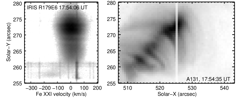
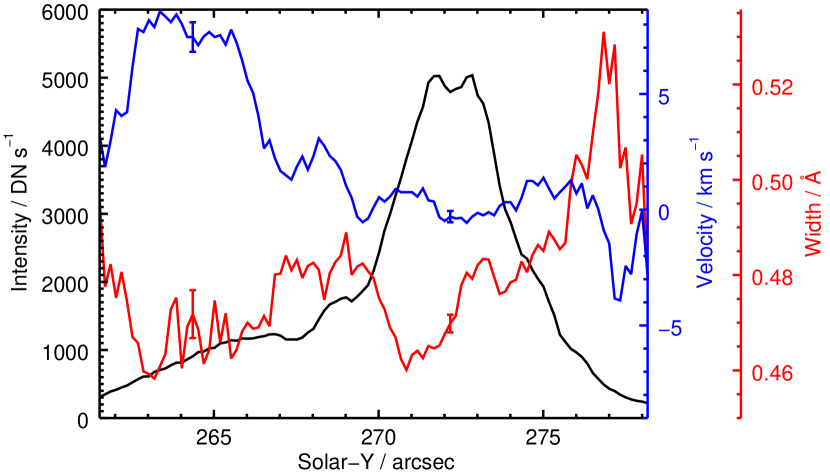
Figure 9: Fe xxi $\lambda$1354.1 Gaussian fit parameters as a function of solar-Y position from R179E6 (17:56:06 UT). The black line shows the line intensity (DN s^-1), the blue line shows LOS velocity (km s^-1), and the red line shows line width (Å). Fitting uncertainties at example locations are indicated.

IRIS has higher spatial resolution than AIA and so allows the sizes of the loop-tops to be determined. There are a number of exposures where quite small features along the IRIS slit can be seen, and an example from R176E1 (17:49:34 UT) is shown in Figure 10a where there are three distinct structures, separated by about 1${{}^{\prime}}{{}^{\prime}}$ (725 km). Averaging the intensity over $\pm 20$ km s^-1 either side of line center gives the intensity profile shown in Figure 10b, and Gaussian fits to the three structures give FWHM values of close to 1${{}^{\prime}}{{}^{\prime}}$. As this is significantly larger than the spatial resolution of the instrument, we consider the structures to be resolved by IRIS. Note that we consider the three structures to be the loop-tops of three distinct flare loops. Other exposures with similar examples of fine-scale structure include R176E2, R178E1 and R178E5.

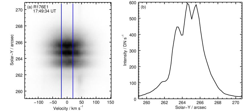
Figure 10: Panel (a) shows an IRIS detector image from 17:49:34 UT, showing strong Fe xxi $\lambda$1354.1 emission. Averaging the intensity over $\pm$ 20 km s^-1 from line center gives the intensity profile with solar-Y position shown in panel (b).

Doschek et al. (1975) demonstrated that the Fe xxi line width decreased with time for one flare. In the present work we have spatially-resolved line width measurements and so we take the median value of the line width, $W$, from each of the rasters R174 to R179, and these are given in Table 2. The median was applied to between 614 and 1177 spatial pixels from these rasters. $W$ can be interpreted as being entirely thermal in origin, in which case a temperature $T_{\rm th}=1.96\times 10^{12}N\,W/\lambda$ K can be derived, where $N$ is the mass number of the emitting element. The values of $T_{\rm th}$ are given in Table 2. This interpretation assumes an isothermal plasma, and the results imply cooling as the flare decays. An alternative interpretation comes from assuming that $\lambda$1354.1 is formed at its temperature of maximum emission ($\log\,T/{\rm K}=7.06$), in which case line broadening beyond the thermal width at this temperature corresponds to non-thermal plasma motions. The non-thermal motions are represented by the velocity $\xi$, given by

$$4\ln 2\left({\lambda\over c}\right)^{2}\xi^{2}=W^{2}-W_{\rm th}^{2},$$ (2)

where $c$ is the speed of light and $W_{\rm th}$ the width at $\log\,T/{\rm K}=7.06$. Table 2 gives the values of $\xi$ assuming this interpretation, and they show non-thermal motions decreasing from 43 to 26 km s^-1 over a six minute period. We note that Doschek et al. (1975) found peak non-thermal motions of 60 km s^-1, falling to 5 km s^-1 about 14 minutes later. In Figure 11 we consider the distribution of widths across two rasters separated by 5 minutes. A cumulative distribution function is used and the total number of spatial pixels was 830 and 1188 for R175 and R179, respectively. The distributions demonstrate that, on the whole, the widths decreased by 0.02 Å over this time, but also that there are more large widths in the earlier raster: for example, 8.8% of spatial pixels have widths $\geq 0.55$ Å for R175, compared to 5.3% for R179. If the measured widths are interpreted purely as thermal widths, then they imply mostly $\log\,T\leq 7.35$ for R175 and $\log\,T\leq 7.25$ for R179. We also note there are very few pixels for which the width is below the thermal width at $\log\,T=7.06$, the temperature of maximum emission of $\lambda$1354.1, which gives confidence that this value is accurate.

Table 2: Average properties derived from Fe xxi $\lambda$1354.1 line widths.

Time	Raster	$W$	$\xi$	$\log\,(T_{\rm th}/{\rm K})$
		(Å)	(km s-1)
17:47:27	R174	0.543	42.8	7.25
17:48:42	R175	0.493	30.0	7.16
17:49:57	R176	0.489	28.9	7.16
17:51:12	R177	0.491	29.6	7.16
17:52.26	R178	0.482	26.9	7.14
17:53:41	R179	0.481	26.3	7.14

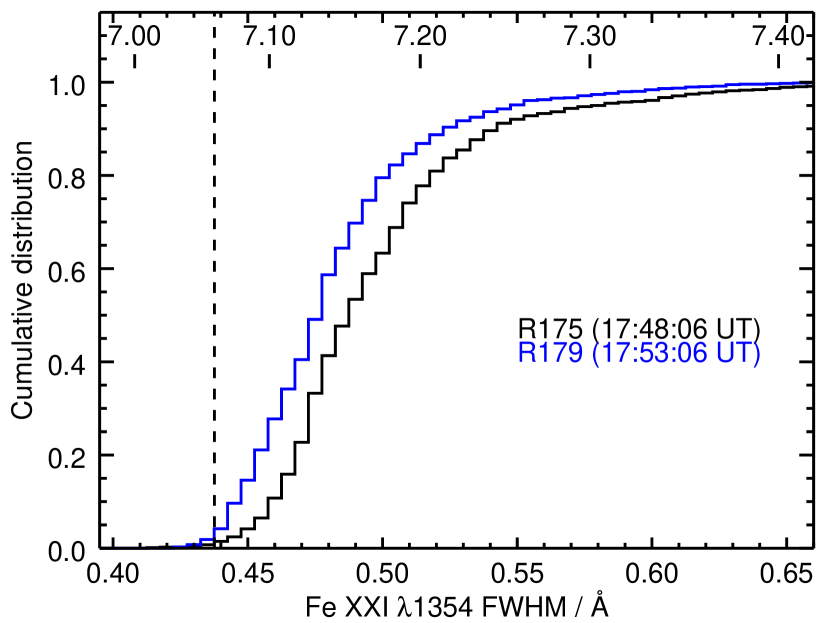
Figure 11: Cumulative distributions of Fe xxi $\lambda$1354.1 line widths from rasters R175 and R179. Logarithmic temperatures corresponding to the widths, assuming they are entirely thermal in origin, are indicated. The vertical dashed line indicates the thermal width at the peak formation temperature ($\log\,T=7.06$) of Fe xxi $\lambda$1354.1.

Away from the ribbons, the Doppler shifts of $\lambda$1354.1 are modest and in fact the IRIS data can be used to estimate a new reference wavelength of 1354.106 Å for the line (Appendix B). Figure 12 shows intensity, velocity and line width maps derived from IRIS raster R179, compared to a co-temporal A131 image. Note that a pixel size of 2${{}^{\prime}}{{}^{\prime}}$ in the X-direction is used for displaying the IRIS images but in reality each column represents only a region 0.33${{}^{\prime}}{{}^{\prime}}$ in the X-direction. The velocity map is derived assuming the rest wavelength of 1354.106 Å for the Fe xxi line (Appendix B). If the value of 1354.064 Å from Feldman et al. (2000) is used, then all velocities would be increased by 9 km s^-1, making the loop arcade almost entirely red-shifted. Figure 12c shows that the region around spatial location (516,260) is red-shifted by around 10–20 km s^-1 and this pattern persists throughout rasters R174 to R179. The northern loop legs generally show a weak blue-shift of a few km s^-1, but with an uncertainty of $\pm 5$ km s^-1 in the rest wavelength of the Fe xxi line (Appendix B) this is not significant.

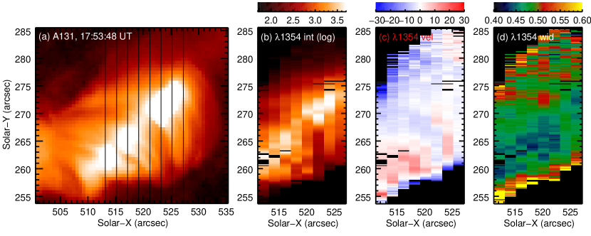
Figure 12: Panel (a) shows the A131 image from 17:53:48 UT with a logarithmic intensity scaling. The brightest parts of the image are saturated, and the eight vertical lines show the locations of the IRIS slit for raster R179. Panels (b), (c) and (d) show the Fe xxi $\lambda$1354.1 intensity (logarithm), velocity and width, in units of DN s^-1, km s^-1, and Å, respectively.

6 Conclusions

In this work we have presented observations of the Fe xxi $\lambda$1354.1 emission line obtained by IRIS during the 2014 March 29 X1 flare. The high spatial resolution and sensitivity of the IRIS instrument allows high temperature ($\approx 10$ MK) plasma to be studied on much smaller spatial scales than previously possible. This has enabled fine structure in the post-flare loop arcade and the flare ribbons to be studied. We distinguish the Fe xxi emission at the flare ribbons from that in the post-flare loop arcade, and we consider that the ribbons represent the footpoints of the post-flare loops.

The variety of Fe xxi profiles at and near the ribbon sites is complex. There are four distinct ribbons, labeled N1, N2, S1 and S2 (see Figure 2), with the brighter N1 and S2 ribbons behaving in the classical manner, being roughly parallel to the polarity inversion line and moving apart with time. These two ribbons both show blue-shifted Fe xxi emission at or close-to the chromospheric ribbon sites, in agreement with the standard flare model. The N2 ribbon sites are partly or wholly compromised by overlying flare loop plasma. The S1 ribbon is unusual as it is of the same polarity as S2 and roughly parallel to it, but it does not move outwards away from the polarity inversion line as S2 does. It also does not show blue-shifted Fe xxi emission, although observations are affected by overlying loop plasma. If we treat the N2 and S1 ribbons as anomalous, then the results for the N1 and S2 ribbons can be summarized as:

1. Of the nine raster positions on the N1 and S2 ribbons, all of them show Fe xxi emission at or close-to the ribbon sites. Eight show Fe xxi blue-shifts of 100 km s^-1 or more.

2. The Fe xxi emission appears at the same time as the ribbon emission for three of the nine positions. There is a delay of 75 seconds in four cases, and a delay of 150 seconds in one case. (The time resolution is restricted by the raster cadence of 75 seconds.)

3. The $\lambda$1354.1 emission when it first appears at the ribbons is mostly compact with a spatial extent $<2$${{}^{\prime}}{{}^{\prime}}$.

4. The S2 ribbon moves southwards by up to 10${{}^{\prime}}{{}^{\prime}}$ during the IRIS raster. Fe xxi emission is found at the previous locations of the ribbon, but the intensity is patchy and the velocity varies. There is some ambiguity as to whether the emission extends along the leg of a single loop, or whether it is low-lying footpoint emission from multiple loops.

5. At some of the ribbon locations, blue-shifted Fe xxi emission remains present until the end of the raster sequence, although the speeds decrease to around 20–60 km s^-1.

6. Studies of $\lambda$1354.1 at the ribbons are compromised by a number of chromospheric emission lines that are found between 1352.5 and 1354.0 Å at the ribbon locations and are comparable in strength to $\lambda$1354.1.

The post-flare loop $\lambda$1354.1 emission began to appear during the impulsive phase of the flare and developed into an extended loop arcade with bright loop-tops. The key results are listed below.

1. The AIA 131 Å filter images, which are dominated by Fe xxi $\lambda$128.7, show that the bright loop-tops have an asymmetric intensity distribution, being more extended on the south-side of the loops.

2. The loop-tops are resolved by IRIS and have sizes of $\geq 1$${{}^{\prime}}{{}^{\prime}}$.

3. IRIS Doppler maps formed from $\lambda$1354.1 show small Doppler shifts in the loop arcade, corresponding to velocities of typically $\leq 10$ km s^-1.

4. Velocities at the loop-tops are close to rest, and the $\lambda$1354.1 width is not significantly enhanced compared to the loop legs.

5. On average there is a slow decrease in the width of the $\lambda$1354.1 emission line of about 0.02 Å over 5 minutes, and there is a greater dispersion of widths near the peak of the flare.

6. Assuming the loop arcade emission is, on average, at rest then a new rest wavelength of $1354.106\pm 0.023$ Å is derived for the Fe xxi line.

The observations generally show agreement with features of the standard solar flare model. In particular Fe xxi is found at the ribbon sites as expected from the intense heating occurring there, and the line is mostly blue-shifted as expected from models of chromospheric evaporation (e.g., Fisher et al., 1985). The connection between the footpoints and the post-flare loops is less clear partly because of the sparse spatial sampling of the rasters. There are a number of exposures such as R179E6 (Figure 9) where blueshifts at the ribbon are observed simultaneously with bright, stationary loop plasma, but a smooth transition from blue-shift to stationary velocity is not common, the intensity often being somewhat patchy at both the footpoint regin and along the loops. This may result from the slit being inclined to the loops’ axes causing multiple loops to be observed in one exposure.

The IRIS instrument has significant flexibility in terms of observation programs and so we highlight here some of the advantages and disadvantages of the observing sequence used for the March 29 flare. Firstly, the eight second exposure time is ideal for studying Fe xxi $\lambda$1354.1 as it yields sufficient signal to study the weak profiles seen at the ribbons, but also the intensities in the post-flare loops do not reach sufficiently high levels that saturation sets in. In particular we note that if the exposure times had been reduced by automatic exposure control then this would have made studying the ribbon emission difficult.

The raster type used for the observation was a “coarse 8-step raster”, which had 2${{}^{\prime}}{{}^{\prime}}$ jumps between slit positions. This enabled a fairly large spatial region to be covered rapidly in X, with the downside of poor sampling. As the IRIS slit did not lie directly along the axes of the post-flare loops, the jumps in X-position generally meant that only small sections of the loops could be observed spectroscopically. In particular the footpoint emission shown in Figure 5 generally terminated abruptly in Y a short distance from the ribbon. A “dense raster”, i.e., step sizes equal to the slit width would have enabled us to check if the variation of footpoint emission with height along the loops could be tracked in the X-direction.

Finally, the wavelength window used for $\lambda$1354.1 is not sufficiently large, with at least one profile (Figure 4c) partially extending beyond the window edge at $-350$ km s^-1. Presently there are five options offered to observers for line-lists, and the “flare line-list” was used for this observation. Extending the 1354 Å window to at least $-500$ km s^-1 from line center is recommended. Also extending the window by around $50$ km s^-1 on the long wavelength side would also be beneficial as O i $\lambda$1355.60 (a line needed for wavelength calibration) is partly out of the window at some locations.

Appendix A Blending lines near Fe XXI $\lambda$1354.1

In flare spectra, particularly near the ribbons, a number of emission lines become prominent that are not normally measurable in the IRIS spectra. Some of these lines compromise measurements of Fe xxi $\lambda$1354.1 and so we discuss these lines here. We note that the large width of $\lambda$1354.1 compared to the cool blending lines means that it is relatively easy to identify $\lambda$1354.1, but the lines affect the measurement of the line parameters (intensity, centroid and width). As discussed in Sect. 4, the ribbons typically appear in chromospheric lines one raster earlier than they do in $\lambda$1354.1, so in Figure 13 we show examples of ribbon spectra without the $\lambda$1354.1 line in order to better display the blending lines. These spectra can be compared with Figure 4 which shows four examples where $\lambda$1354.1 is present.

The spectrum in Figure 13a is the most common type of ribbon spectrum, with two lines of Si ii and one of Fe ii becoming comparable in intensity to C i $\lambda$1354.29. The two Si ii lines often show interesting dynamics at the flare ribbons, with broad long-wavelength wings extending up to 150 km s^-1. The broad wings can be confused with Fe xxi emission, but the presence of two Si ii lines enables the Si ii components to be easily identified.

Figure 13b shows a spectrum about 1${{}^{\prime}}{{}^{\prime}}$ from a ribbon where a pair of very close lines are found at 1353.32 and 1353.39 Å. By comparing the intensity distribution along the slit, these lines show similar behavior to a pair of lines at 1333.48 and 1333.80 Å that are known to be H₂ lines fluoresced by Si iv (Bartoe et al., 1979). Another possibility is that they are CO lines, although they are not listed by Jordan et al. (1979).

An unusual spectrum is seen in a few of the flare exposures and an example is shown in Figure 13c. Two lines at 1353.55 and 1354.19Å are particularly prominent and are striking because of their very narrow widths of $\approx 0.045$ Å. The lines have a very different intensity distribution along the slit compared to the atomic lines or H₂ and there are many similar lines in the spectrum including a distinctive group of 5–6 lines between 1402.0 and 1402.5 Å, on the short wavelength side of Si iv $\lambda$1402.77.

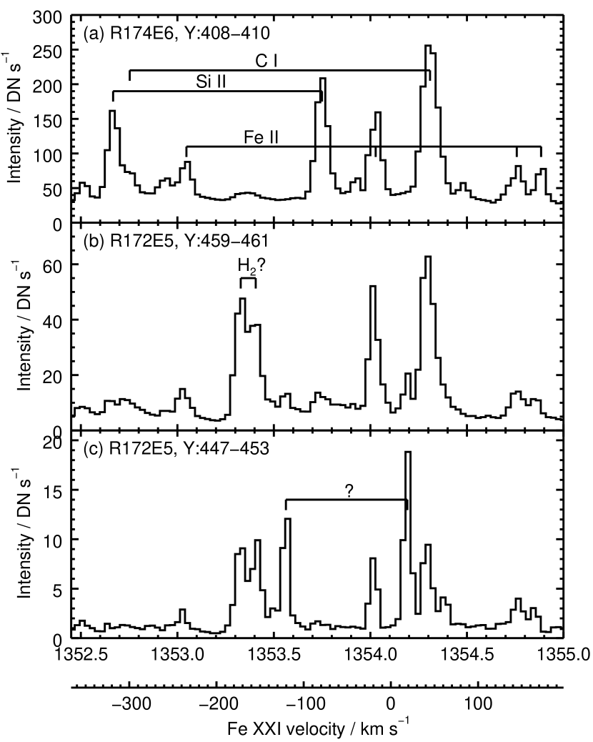
Figure 13: Three examples of IRIS spectra at or in the vicinity of flare ribbons. The Y-pixel ranges over which the spectra are averaged are indicated.

Appendix B The rest wavelength of Fe XXI $\lambda$1354.1

For creating velocity maps from Fe xxi $\lambda$1354.1 it is necessary to set an absolute wavelength scale. For this we use O i $\lambda$1355.60 which is a narrow chromospheric line that demonstrates only small Doppler shifts in rasters. The reference wavelength for this line is 1355.5977 Å, which is a calculated value with an accuracy estimated at 0.5 mÅ (Eriksson & Isberg, 1968). As described in Sect. 5 we fit three Gaussians to the wavelength window containing Fe xxi $\lambda$1354.1, one of which represents the O i line.

We used rasters R177–179 to determine the Fe xxi wavelength as these show strong emission from the post-flare loops, and the line is mostly close to the rest wavelength. We restrict analysis to those spatial pixels for which the $\lambda$1354.1 line width is between 0.42 and 0.55 Å, i.e., close to the thermal width of 0.43 Å, the integrated intensity is $\geq$ 50 DN, and the reduced $\chi^{2}$ value for the fit is $\leq$ 1.5. These restrictions remove pixels for which the line shows unusual dynamics, is weak, or has a poor fit. For these spatial pixels we take the set of O i centroids, measured through a Gaussian fit, and compute the mean and standard deviations. These values are shown in Table 3. Similarly the mean and standard deviation of the Fe xxi wavelengths are computed. We correct the derived Fe xxi wavelength by the difference between the derived and reference O i wavelengths, giving the rest Fe xxi wavelengths shown in Table 3. The uncertainty has been obtained by adding in quadrature the standard deviations of the measured Fe xxi and O i wavelengths, and the uncertainity in the O i reference wavelength. Combining these results gives a final rest wavelength of $1354.106\pm 0.023$ Å, which we adopt in the present work.

We note that there is a significant discrepancy with the value of $1354.064\pm 0.020$ Å from Feldman et al. (2000). If this value is correct, then it implies that the post-flare loops in the present observation are, on average, red-shifted by 9 km s^-1.

Table 3: Measured wavelengths for O i and Fe xxi.

Raster	O i	Fe xxi
R177	$1355.6204\pm 0.0090$	$1354.106\pm 0.023$
R178	$1355.6205\pm 0.0080$	$1354.106\pm 0.022$
R179	$1355.6211\pm 0.0078$	$1354.107\pm 0.023$

References

- Acton et al. (1992) Acton, L. W., et al. 1992, PASJ, 44, L71
- Ayres et al. (2003) Ayres, T. R., Brown, A., Harper, G. M., Osten, R. A., Linsky, J. L., Wood, B. E., & Redfield, S. 2003, ApJ, 583, 963
- Bartoe et al. (1979) Bartoe, J.-D. F., Brueckner, G. E., Nicolas, K. R., Sandlin, G. D., Vanhoosier, M. E., & Jordan, C. 1979, MNRAS, 187, 463
- Benz (2008) Benz, A. O. 2008, Living Reviews in Solar Physics, 5
- Cheng et al. (1979) Cheng, C.-C., Feldman, U., & Doschek, G. A. 1979, ApJ, 233, 736
- De Pontieu et al. (2014) De Pontieu, B., et al. 2014, Sol. Phys., 289, 2733
- Del Zanna et al. (2006) Del Zanna, G., Berlicki, A., Schmieder, B., & Mason, H. E. 2006, Sol. Phys., 234, 95
- Dere et al. (1997) Dere, K. P., Landi, E., Mason, H. E., Monsignori Fossi, B. C., & Young, P. R. 1997, A&AS, 125, 149
- Doschek et al. (1975) Doschek, G. A., Dere, K. P., Sandlin, G. D., Vanhoosier, M. E., Brueckner, G. E., Purcell, J. D., Tousey, R., & Feldman, U. 1975, ApJ, 196, L83
- Doyle & Phillips (1992) Doyle, J. G., & Phillips, K. J. H. 1992, A&A, 257, 773
- Eriksson & Isberg (1968) Eriksson, K. B. S., & Isberg, H. B. S. 1968, Ark. Fys., 37, 221
- Feldman et al. (2000) Feldman, U., Curdt, W., Landi, E., & Wilhelm, K. 2000, ApJ, 544, 508
- Feldman et al. (1994) Feldman, U., Seely, J. F., Doschek, G. A., Strong, K. T., Acton, L. W., Uchida, Y., & Tsuneta, S. 1994, ApJ, 424, 444
- Fisher et al. (1985) Fisher, G. H., Canfield, R. C., & McClymont, A. N. 1985, ApJ, 289, 414
- Handy et al. (1999) Handy, B. N., et al. 1999, Sol. Phys., 187, 229
- Heinzel & Kleint (2014) Heinzel, P., & Kleint, L. 2014, ApJ, 794, L23
- Innes et al. (2001) Innes, D. E., Curdt, W., Schwenn, R., Solanki, S., Stenborg, G., & McKenzie, D. E. 2001, ApJ, 549, L249
- Innes et al. (2003a) Innes, D. E., McKenzie, D. E., & Wang, T. 2003a, Sol. Phys., 217, 267
- Innes et al. (2003b) Innes, D. E., McKenzie, D. E., & Wang, T. 2003b, Sol. Phys., 217, 247
- Jakimiec et al. (1998) Jakimiec, J., Tomczak, M., Falewicz, R., Phillips, K. J. H., & Fludra, A. 1998, A&A, 334, 1112
- Jordan et al. (1979) Jordan, C., Bartoe, J.-D. F., Brueckner, G. E., Nicolas, K. R., Sandlin, G. D., & Vanhoosier, M. E. 1979, MNRAS, 187, 473
- Judge et al. (2014) Judge, P. G., Kleint, L., Donea, A., Sainz Dalda, A., & Fletcher, L. 2014, ArXiv e-prints
- Kliem et al. (2002) Kliem, B., Dammasch, I. E., Curdt, W., & Wilhelm, K. 2002, ApJ, 568, L61
- Landi et al. (2003) Landi, E., Feldman, U., Innes, D. E., & Curdt, W. 2003, ApJ, 582, 506
- Landi et al. (2013) Landi, E., Young, P. R., Dere, K. P., Del Zanna, G., & Mason, H. E. 2013, ApJ, 763, 86
- Lemen et al. (2012) Lemen, J. R., et al. 2012, Sol. Phys., 275, 17
- Maran et al. (1994) Maran, S. P., et al. 1994, ApJ, 421, 800
- Mason et al. (1986) Mason, H. E., Shine, R. A., Gurman, J. B., & Harrison, R. A. 1986, ApJ, 309, 435
- Milligan et al. (2006) Milligan, R. O., Gallagher, P. T., Mathioudakis, M., Bloomfield, D. S., Keenan, F. P., & Schwartz, R. A. 2006, ApJ, 638, L117
- O’Dwyer et al. (2010) O’Dwyer, B., Del Zanna, G., Mason, H. E., Weber, M. A., & Tripathi, D. 2010, A&A, 521, A21
- Sandlin et al. (1977) Sandlin, G. D., Brueckner, G. E., & Tousey, R. 1977, ApJ, 214, 898
- Teriaca et al. (2003) Teriaca, L., Falchi, A., Cauzzi, G., Falciani, R., Smaldone, L. A., & Andretta, V. 2003, ApJ, 588, 596
- Teriaca et al. (2006) Teriaca, L., Falchi, A., Falciani, R., Cauzzi, G., & Maltagliati, L. 2006, A&A, 455, 1123
- Tian et al. (2014) Tian, H., Li, G., Reeves, K. K., Raymond, J. C., Guo, F., Liu, W., Chen, B., & Murphy, N. A. 2014, ArXiv e-prints
- Wang et al. (2003a) Wang, T. J., Solanki, S. K., Curdt, W., Innes, D. E., Dammasch, I. E., & Kliem, B. 2003a, A&A, 406, 1105
- Wang et al. (2003b) Wang, T. J., Solanki, S. K., Innes, D. E., Curdt, W., & Marsch, E. 2003b, A&A, 402, L17
- Watanabe et al. (2011) Watanabe, H., Vissers, G., Kitai, R., Rouppe van der Voort, L., & Rutten, R. J. 2011, ApJ, 736, 71
- Xu et al. (2012) Xu, Y., Cao, W., Jing, J., & Wang, H. 2012, ApJ, 750, L7
- Young (2013) Young, P. R. 2013, EIS Software Note No. 16, ver. 2.5
- Young et al. (2013) Young, P. R., Doschek, G. A., Warren, H. P., & Hara, H. 2013, ApJ, 766, 127