Iso-Flux Tension Propagation Theory of Driven Polymer Translocation: The Role of Initial Configurations

Abstract

We investigate the dynamics of pore-driven polymer translocation by theoretical analysis and molecular dynamics (MD) simulations. Using the tension propagation theory within the constant flux approximation we derive an explicit equation of motion for the tension front. From this we derive a scaling relation for the average translocation time $\tau$, which captures the asymptotic result $\tau\propto N_{0}^{1+\nu}$, where $N_{0}$ is the chain length and $\nu$ is the Flory exponent. In addition, we derive the leading correction-to-scaling term to $\tau$ and show that all terms of order $N_{0}^{2\nu}$ exactly cancel out, leaving only a finite-chain length correction term due to the effective pore friction, which is linearly proportional to $N_{0}$. We use the model to numerically include fluctuations in the initial configuration of the polymer chain in addition to thermal noise. We show that when the cis side fluctuations are properly accounted for, the model not only reproduces previously known results but also considerably improves the estimates of the monomer waiting time distribution and the time evolution of the translocation coordinate $s(t)$, showing excellent agreement with MD simulations.

I Introduction

Polymer translocation has in less that 20 years become one of the most active research areas in soft matter biological physics. Since the initial experimental work of Kasianowicz et al. kasi1996 on RNA translocation through $\alpha$-hemolysin channels, the interest in the potential technological applications such as gene therapy, drug delivery and rapid DNA sequencing has motivated a steady flow of experimental and theoretical research meller2003 ; Muthukumar_book ; Milchev_JPCM ; Tapio_review ; schadt2010 ; branton2008 ; storm2005 ; chuang2001 ; kantor2004 ; sung1996 ; metzler2003 ; muthu1999 ; sakaue2007 ; sakaue2008 ; sakaue2010 ; saito2011 ; rowghanian2011 ; luo2008 ; saito2012a ; saito2012b ; grosberg2006 ; luo2009 ; dubbeldam2011 ; dubbeldam2007 ; bhatta2009 ; bhatta2010 ; lehtola2009 ; lehtola2010 ; ikonen2012a ; ikonen2012b ; ikonen2013 . Of particular interest is the case of the pore-driven polymer translocation, where the segment of the polymer inside the pore is driven by an electric field. Unlike the case of unbiased translocation, where the polymer supposedly has enough time to equilibrate in some limits unbiased_Slater_1 ; unbiased_Slater_2 ; unbiased_Slater_3 ; unbiased_Polson the driven translocation problem is inherently a far-from-equilibrium process bhatta2009 ; bhatta2010 ; lehtola2009 ; lehtola2010 .

In the recent years, significant advance has been made in the theoretical basis of driven polymer translocation. It is now understood that the dynamics of driven translocation is dominated by the drag of the cis side chain, with leading order corrections stemming from the friction of the pore ikonen2012a ; ikonen2012b ; ikonen2013 , with the trans side suspected to have only a minor effect on the whole process ikonen2012b ; dubbeldam2014 ; suhonen2014 . To evaluate the contribution from the cis side drag, one must study the non-equilibrium time evolution of the chain configurations. The basic picture is that of two domains, with the chain divided into mobile and immobile parts, where only the segments belonging into the mobile part contribute to the drag. In the simplest description, the process can be viewed as a sequential straightening of loops, where the loops between a given segment and the pore need to be pulled straight before the segment can experience the force and become mobile grosberg2006 ; dimarzio1979 ; ikonen2013 . Based on this picture, the scaling form $\tau\propto N_{0}^{\alpha}$ for the average translocation time $\tau$ as a function of chain length $N_{0}$ can be derived with scaling arguments ikonen2013 , giving $\tau(N_{0})=c_{1}N_{0}^{1+\nu}+c_{2}\tilde{\eta}_{p}N_{0}$, where $c_{1}$ and $c_{2}$ are constants. Here the first term is due to the cis side drag and contains the Flory exponent $\nu$ that characterizes the initial shape of the chain, given by the end-to-end distance $R\propto N_{0}^{\nu}$. The latter term is due to the interaction of the pore and the polymer, the strength of which is given by the effective pore friction $\tilde{\eta}_{p}$.

Thermal fluctuations from the solvent introduce both undulations to the shape of the chain and randomness into the effective driving force. Using blob theory, it is possible to describe the shape of the mobile part and the propagation of the boundary between the mobile and immobile parts self-consistently sakaue2007 ; sakaue2008 ; sakaue2010 ; saito2011 ; rowghanian2011 ; dubbeldam2011 ; saito2012a ; saito2012b ; ikonen2012a ; ikonen2012b . Asymptotic analysis of this tension propagation theory also gives the long chain limit of the translocation time as $\tau=c_{1}N_{0}^{1+\nu}$, similar to the simple scaling arguments ikonen2013 . Numerical analysis has shown that the finite chain length effects due to the pore friction persist for extremely long chains, and that they are responsible for the scatter in the reported values of the scaling exponent $\alpha$ ikonen2012a ; ikonen2012b ; ikonen2013 .

With numerical methods, one may also consider the effect of thermal fluctuations to the driving force. Previous results indicate that the randomness of the effective force alone is insufficient to explain the fluctuations observed in molecular dynamics simulations ikonen2012b . Saito and Sakaue have proposed that for large driving forces the uncertainty in the initial configurations would determine the distribution of the translocation time saito2012a .

In this paper, our main aim is to investigate the influence of the uncertainty in the initial chain configuration to translocation dynamics by introducing stochasticity to the initial chain configuration at the cis side. This is based on using the Brownian dynamics - tension propagation (BDTP) framework introduced in Refs. ikonen2012a ; ikonen2012b . We modify this approach by deriving the tension propagation (TP) equations by assuming a constant monomer flux on the mobile part of the chain in the cis side. This formalism leads to an explicit equation of motion for the velocity of the tension front and eliminates the need of the original BDTP model to include an approximate initial velocity profile to ensure the conservation mass. In addition, the model allows us to derive a finite-size scaling form for the average translocation time, which is in agreement with ansatz of Ref. ikonen2013 .

This paper is organized as follows: In Sec. ​II we demonstrate how to model driven translocation based on the iso-flux Brownian dynamics tension propagation (IFTP) formalism. Section ​III is devoted to deriving the finite-size scaling form for the translocation time. In Sec. ​IV it is shown how the initial configurations can be incorporated into the theory. Secs. ​V.1, V.2, V.3 and V.4 present the results on the average of the translocation time, waiting time distribution, distribution of the translocation time and time evolution of the translocation coordinate, respectively. Finally, the conclusions and discussion are in Sec. ​VI.

II Model

For brevity, we use dimensionless units denoted by tilde as $\tilde{Y}\equiv Y/Y_{u}$, with the units of time $t_{u}\equiv\eta a^{2}/(k_{B}T)$, length $s_{u}\equiv a$, velocity $v_{u}\equiv a/t_{u}=k_{B}T/(\eta a)$, force $f_{u}\equiv k_{B}T/a$, friction $\Gamma_{u}\equiv\eta$, and monomer flux $\phi_{u}\equiv k_{B}T/(\eta a^{2})$, where $k_{B}$ is the Boltzmann constant, $T$ is the temperature of the system, $a$ is the segment length, and $\eta$ is the solvent friction per monomer.

Figure 1: (a) A schematic picture of the translocation process during propagation stage for the trumpet regime. The driving force $f$ acts on polymer at the pore towards the trans side. The length of polymer is $N_{0}$ and the number of beads that have already been translocated into the trans side is denoted by $\tilde{s}$. The number of beads influenced by the tension in the cis side is $\tilde{l}+\tilde{s}$ which is less than the number of total beads in the polymer $N_{0}$ during propagation stage. The location of the last blob is determined by $\tilde{R}$. (b) The translocation process when the tension front reaches the chain end and after it for the trumpet regime (post propagation stage). (c) The same as (a) but for the stem-flower regime. $\tilde{\tau}_{\textrm{tp,T}}$ and $\tilde{\tau}_{\textrm{tp,SF}}$ define the propagation times in the trumpet and stem-flower regimes, respectively, as in Eq. ​(6).

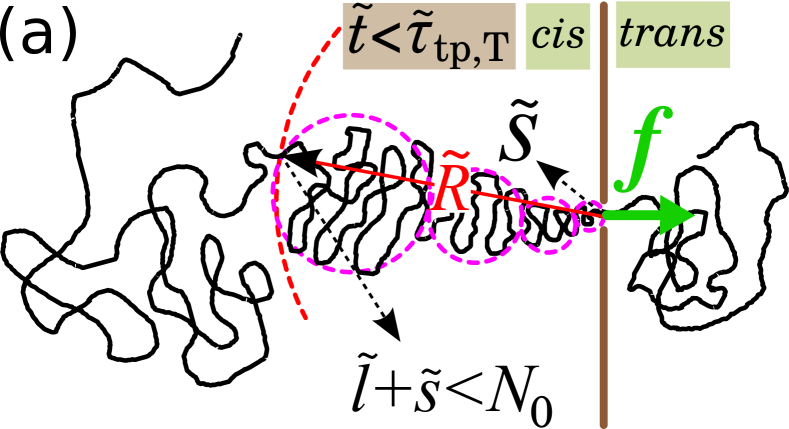
As a basic framework we use Brownian dynamics (BD) in the overdamped limit, similar to Refs. ikonen2012a ; ikonen2012b . The BD equation is written for the translocation coordinate $\tilde{s}$ that gives the length of the chain on the trans side. The equation reads as

$$\tilde{\Gamma}(\tilde{t})\frac{d\tilde{s}}{d\tilde{t}}=(1-\gamma^{\prime})\bigg{[}\frac{1}{N_{0}-\tilde{s}}-\frac{1}{\tilde{s}}\bigg{]}+\tilde{f}+\tilde{\zeta}(\tilde{t})\equiv\tilde{f}_{\textrm{tot}},$$ (1)

where $\tilde{\Gamma}$ is the effective friction, and $\tilde{\xi}(\tilde{t})$ is Gaussian white noise which satisfies $\langle\xi(t)\rangle=0$ and $\langle\xi(t)\xi(t)\rangle=2\Gamma k_{B}T\delta(t-t^{\prime})$, $\gamma^{\prime}$ is the surface exponent ($\gamma^{\prime}=0.5$ for ideal chains, and $\approx~{}0.95,\approx~{}0.69$ for self-avoiding chains in two and three dimensions, respectively), $N_{0}$ is the total number of beads in the chain (the contour length of the chain is $L=aN_{0}$), $\tilde{f}$ is the external driving force and $\tilde{f}_{\textrm{tot}}$ is the total force. The effective friction $\tilde{\Gamma}$ depends on the pore friction $\tilde{\eta}_{p}$ and the drag force on the cis side. As the dynamical trans side contribution to the dynamics has been shown to be insignificant ikonen2012a ; ikonen2012b ; ikonen2013 ; dubbeldam2014 ; suhonen2014 , we absorb it into the constant pore friction $\tilde{\eta}_{p}$. The dynamics of the cis side is solved with the TP equations.

To derive the TP equations, we use arguments similar to Rowghanian et al. rowghanian2011 . We assume that the flux $\tilde{\phi}\equiv d\tilde{s}/d\tilde{t}$ of monomers on the mobile domain of the cis side and through the pore is constant in space, but evolves in time. The boundary between the mobile and immobile domains, the tension front, is located at distance $\tilde{x}=-\tilde{R}(\tilde{t})$ from the pore. Inside the mobile domain, the external driving force is mediated by the chain backbone from the pore at $\tilde{x}=0$ all the way to the last mobile monomer $N$ located at the tension front. The magnitude of the tension force at distance $\tilde{x}$ can be calculated by considering the force-balance relation for the differential element $d\tilde{x}$ that is located between $\tilde{x}$ and $\tilde{x}+d\tilde{x}$. By integrating the force-balance relation over the distance from the pore entrance to $\tilde{x}$, the tension force can be obtained as $\tilde{f}(\tilde{x},\tilde{t})=\tilde{f}_{0}-\tilde{\phi}(\tilde{t})\tilde{x}$ (see Appendix A for details). Here $\tilde{f}_{0}\equiv\tilde{f}_{\textrm{tot}}-\tilde{\eta}_{p}\tilde{\phi}(\tilde{t})$ is the force at the pore entrance.

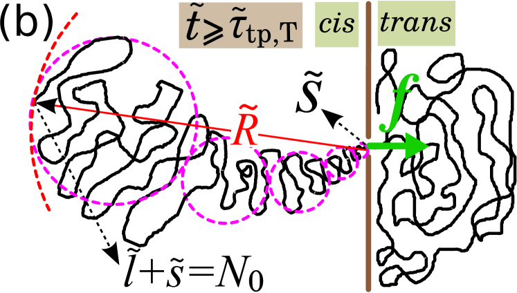
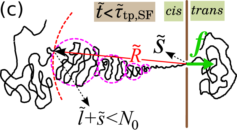
Closer to the tension front the mediated force is therefore smaller, as it is diminished by the drag of all the preceding monomers. According to blob theory, the chain then assumes a trumpet-like shape with the narrow end closer to the pore, such as shown in Figs. 1 ​(a) and (b). For a moderate external driving force, i.e. $N_{0}^{-\nu}\ll\tilde{f}_{0}\ll 1$, the monomer density at the pore is greater than unity, and the shape of the chain resembles a trumpet. This is classified as a trumpet (TR) regime. For a stronger external driving force, $1\ll\tilde{f}_{0}\ll N_{0}^{\nu}$, the force is large enough to completely straighten a small part of the chain. This part is called the stem, while the part following it is called the flower, corresponding to the stem-flower (SF) regime (see Fig. 1 ​(c)). In both regimes the tension front is located at the farthest blob from the pore as depicted in Fig. 1.

Integration of the force balance equation over the mobile domain gives an expression for the monomer flux as a function of the force and the linear size of the mobile domain as

$$\tilde{\phi}(\tilde{t})=\frac{\tilde{f}_{\textrm{tot}}(\tilde{t})}{\tilde{\eta}_{\textrm{p}}+\tilde{R}(\tilde{t})}.$$ (2)

Equation (1) and the definition of the flux, $\tilde{\phi}\equiv d\tilde{s}/d\tilde{t}$, can be then used to find the expression for the effective friction as

$$\tilde{\Gamma}(\tilde{t})=\tilde{R}(\tilde{t})+\tilde{\eta}_{p}.$$ (3)

Equations (1), (2) and (3) determine the time evolution of $\tilde{s}$, but the full solution still requires the knowledge of $\tilde{R}(\tilde{t})$. The derivation of the equation of motion of $\tilde{R}(\tilde{t})$ is done separately for the propagation and post propagation stages. In the propagation stage, the tension has not reached the final monomer in Fig. 1 ​(a). Here the propagation of the tension front into the immobile domain is determined by the geometric shape of the immobile domain. In practice, one uses the scaling relation of the end-to-end distance of the self-avoiding chain to arrive at the closure relation $\tilde{R}=A_{\nu}N^{\nu}$, where $A_{\nu}$ is a constant prefactor and $N$ is the last monomer inside the tension front. As shown in Appendix B, one can then derive an equation of motion for the tension front as

$$\dot{\tilde{R}}(\tilde{t})=\frac{\nu A_{\nu}^{\frac{1}{\nu}}\tilde{R}(\tilde{t})^{\frac{\nu-1}{\nu}}\big{[}({\cal{L}}_{\textrm{a}}+{\cal{G}}_{\textrm{a}})\times\dot{\tilde{f}}_{\textrm{tot}}(\tilde{t})+\tilde{\phi}(\tilde{t})\big{]}}{1+\nu A_{\nu}^{\frac{1}{\nu}}\tilde{R}(\tilde{t})^{\frac{\nu-1}{\nu}}{\cal{L}}_{\textrm{a}}\times\tilde{\phi}(\tilde{t})},$$ (4)

where ${\cal{L}}_{\textrm{a}}$ and ${\cal{G}}_{\textrm{a}}$ are functions of $\tilde{\phi}$, $\tilde{\eta}_{p}$ and $\nu$, $\dot{\tilde{f}}_{\textrm{tot}}$ is the time derivative of $\tilde{f}_{\textrm{tot}}$, and the subscript ”a” in ${\cal{L}}_{\textrm{a}}$ and ${\cal{G}}_{\textrm{a}}$ stands for the trumpet regime as $\textrm{T}_{+}$ and $\textrm{T}_{-}$ correspond to positive and negative values of $\tilde{\phi}$ respectively, and for the stem-flower regime as SF.

In the post propagation stage in Fig. 1 ​(b), every monomer on the cis is affected by the tension. Therefore, we have the condition $N=N_{0}$. Since $N$ is also equal to the number of monomers already translocated, $\tilde{s}$, plus the number of monomers currently mobile on the cis side, $\tilde{l}$, the correct closure relation for the post propagation stage is $\tilde{l}+\tilde{s}=N_{0}$. The equation of motion for the tension front is then derived as

$$\dot{\tilde{R}}(\tilde{t})=\frac{({\cal{L}}_{\textrm{a}}+{\cal{G}}_{\textrm{a}})\dot{\tilde{f}}_{\textrm{tot}}(\tilde{t})+\tilde{\phi}(\tilde{t})}{\tilde{\phi}(\tilde{t})\times{\cal{L}}_{\textrm{a}}},$$ (5)

which is demonstrated in Appendix B.

The self-consistent solution for the model in the propagation stage can be obtained from Eqs. ​(1), (2), (3) and (4). Correspondingly, in the post propagation one uses the set of Eqs. ​(1), (2), (3) and (5).

III Scaling of translocation time

To obtain some analytical results, it is useful to consider the approximation of constant force, $\tilde{f}_{\textrm{tot}}=\tilde{f}$. Then Eq. ​(2) reduces to $\tilde{\phi}(\tilde{t})=\tilde{f}/\left(\tilde{R}(\tilde{t})+\tilde{\eta}_{p}\right)$. In the stem-flower and trumpet regimes, the number of mobile monomers on the cis side is given by $\tilde{l}_{\textrm{SF}}=\tilde{R}+C_{\nu}\tilde{\phi}^{-1}$, and $\tilde{l}_{\textrm{T}}=\frac{\nu}{2\nu-1}\tilde{\phi}^{(\nu-1)/\nu}\tilde{R}^{(2\nu-1)/\nu}$, respectively, where $C_{\nu}=(1-\nu)/(2\nu-1)$. This together with the conservation of mass, $N=\tilde{s}+\tilde{l}$, allows one to solve the propagation time $\tilde{\tau}_{\mathrm{tp}}$ by integration of $N$ from $0$ to $N_{0}$. The result is

$$\tilde{\tau}_{\mathrm{tp,a}}=\frac{1}{\tilde{f}}\bigg{[}\int_{0}^{N_{0}}\tilde{R}(N)dN+\tilde{\eta}_{p}N_{0}\bigg{]}-\Delta\tilde{\tau}_{\mathrm{a}},$$ (6)

where the subscript ”a” denotes SF and T, and

$$\Delta\tilde{\tau}_{\mathrm{SF}}= \left(\frac{1}{\tilde{f}}+\frac{C_{\nu}}{\tilde{f}^{2}}\right)\left[\frac{1}{2}\tilde{R}^{2}(N_{0})+\tilde{\eta}_{p}\tilde{R}(N_{0})\right],$$

$$\Delta\tilde{\tau}_{\mathrm{T}}= \tilde{f}^{-\frac{1}{\nu}}\bigg{[}\int_{0}^{\tilde{R}(N_{0})}d\tilde{R}~{}\tilde{R}^{1-\frac{1}{\nu}}\big{(}\tilde{R}+\tilde{\eta}_{\textrm{p}}\big{)}^{\frac{1}{\nu}}$$

$$+C_{\nu}\int_{0}^{\tilde{R}(N_{0})}d\tilde{R}~{}\tilde{R}^{2-\frac{1}{\nu}}\big{(}\tilde{R}+\tilde{\eta}_{\textrm{p}}\big{)}^{\frac{1}{\nu}-1}\bigg{]}.$$ (7)

In the post propagation stage, one sets the condition $dN/d\tilde{t}=0$ and integrates $\tilde{R}$ from $\tilde{R}(N_{0})$ to $0$. The result for the post-propagation time $\tilde{\tau}_{\mathrm{pp}}$ is

$$\tilde{\tau}_{\mathrm{pp,a}}=\Delta\tilde{\tau}_{\mathrm{a}}.$$ (8)

The time over the whole translocation process is then given by

$$\tilde{\tau}_{\textrm{a}}=\tilde{\tau}_{\mathrm{tp,a}}+\tilde{\tau}_{\mathrm{pp,a}} =\frac{1}{\tilde{f}}\left[\int_{0}^{N_{0}}\tilde{R}(N)dN+\tilde{\eta}_{p}N_{0}\right]$$

$$=\frac{A_{\nu}}{(1+\nu)\tilde{f}}N_{0}^{1+\nu}+\frac{\tilde{\eta}_{p}}{\tilde{f}}N_{0}.$$ (9)

This is a remarkable result in the sense that although terms proportional to $N_{0}^{2\nu}$ appear in the intermediate steps, as predicted for instance in Refs. ​saito2012a ; dubbeldam2011 , the terms are canceled out in the expression for the total translocation time. This result is in agreement with the previously proposed scaling analysis and MD simulations in Ref. ikonen2013 .

IV Distribution of Initial Configurations

In previous works with the BDTP model, an average end-to-end distance $\tilde{R}=A_{\nu}N^{\nu}$ was used with a constant coefficient $A_{\nu}=1.15$ in 3D ikonen2012a ; ikonen2012b . To study the influence of initial configurations on the translocation process we employ a new probability distribution function to sample the end-to-end distance of the chain. To obtain the distribution, we have done Langevin-thermostatted molecular dynamics simulations of self-avoiding chains tethered onto an impenetrable wall and calculated the end-to-end distance of chain. We simulated several chain lengths up to $N_{0}=321$, with standard Kremer-Grest bead-spring model of the chain and other parameters typically used in the MD simulations. For detailed account of the simulation method and the parameters, see e.g. Refs. ikonen2012a ; ikonen2012b .

The distribution of the end-to-end distances for $N_{0}=321$ is shown in Fig. ​2. An analytical function was fitted to the cumulative distribution function constructed from the data by minimizing the squared error with the conditions that the total probability and the second moment are equal to unity. The obtained analytical probability distribution function can be written as

$$P(y)=A~{}\!y^{B}{\textrm{exp}}\big{[}Cy^{D}],$$ (10)

where $A=0.4252$, $B=1.0310$, $C=-1.4417$, $D=2.6203$, and $y$ is the normalized end-to-end distance $y=\tilde{R}/\langle\tilde{R}\rangle$. The fitted function was also compared to MD data of shorter chains ($N_{0}=81$ and $N_{0}=161$) with a Kolmogorov-Smirnov test, showing that within 99 % statistical confidence the shorter chains follow the same distribution for the normalized end-to-end distance.

Figure 2: MD data for the probability distribution function multiplied by $4\pi y^{2}$ (yellow bars), with fitting to the MD data shown as a black line. The fitting curve is $4\pi y^{2}P(y)$ where $P(y)=4\pi y^{2}A~{}\!y^{B}{\textrm{exp}}\big{[}Cy^{D}]$ and $A=0.4252$, $B=1.0310$, $C=-1.4417$, $D=2.6203$.

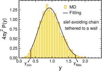
Using Eq. ​(10) one can sample over many different initial configurations. By choosing $y$ from the probability distribution function in Eq. ​(10) and redefining $\tilde{R}$ as $\tilde{R}=A_{\nu}(y)~{}N_{0}^{\nu}$, one can incorporate an approximate distribution of $\tilde{R}$ into the TP theory through $A_{\nu}(y)=yA_{\nu}$. For numerical reasons we have covered the range $y_{\textrm{min}}<y<y_{\textrm{max}}$, where $y_{\textrm{min}}=0.356$ and $y_{\textrm{max}}=1.718$. This is justified because 97 $\%$ of the area below the curve in Fig. ​2 is still covered by choosing these cutoffs.

V Results

V.1 Average translocation time

The most fundamental property related to the translocation process is the average translocation time $\tilde{\tau}$. According to the analysis of Section III, the translocation time $\tilde{\tau}$ depends on the chain length $N_{0}$ as

$$\tilde{\tau}\equiv c_{1}(\tilde{f},\nu,A_{\nu})~{}N_{0}^{1+\nu}+c_{2}(\tilde{f})~{}\tilde{\eta}_{\textrm{p}}N_{0}.$$ (11)

Written in the conventional scaling form, $\tilde{\tau}\propto N_{0}^{\alpha}$, it is evident that the effective exponent $\alpha$ is a function of chain length due to the correction-to-asymptotic-scaling term in Eq. (11).

To illustrate this behavior, we have solved the model numerically. For parameter values $f=5.0$, $k_{B}T=1.2$, $\eta=0.7$, and pore frictions $\eta_{\textrm{p}}=1.0,2.0,5.0$ and 10.0, the translocation time as a function of chain length is shown in Fig. ​3 ​(a). Here we have used a fixed value $A_{\nu}=1.15$ and we have set the stochastic term $\zeta$ in the force to zero in order to be able to simulate chain lengths up to $N_{0}\approx 10^{6}$. For short chains, there is a clear dependence in the slope on the pore friction. For the long chains, this dependence dies off as the asymptotic limit of $\alpha=1+\nu$ is reached.

Figure 3: (a) The translocation time as a function of the chain length, $N_{0}$, for fixed values of the force, $f=5.0$, and $A_{\nu}=1.15$ for various values of $\eta_{\textrm{p}}$. The effective exponent for the shortest chain, $N_{0}=40$, and pore friction $\eta_{\textrm{p}}=1.0$ is $1.516$, while for highest value of pore friction $\eta_{\textrm{p}}=10.0$ it is $1.260$. The effective exponent for the longest chain, $N_{0}=5\times 10^{5}$ is $1.588$. (b) The effective exponent $\alpha(N_{0})$ as a function of the chain length for various values of pore friction $\eta_{\textrm{p}}$, and the rescaled exponent that is also plotted as a function of chain length for various $\eta_{\textrm{p}}$. As can be seen, the rescaled exponent curves for different values of $\eta_{\textrm{p}}$ collapse on a single master curve, i.e. $\alpha^{{\dagger}}(N_{0})=1+\nu$, as denoted by rescaled data in the figure. (c) The normalized translocation time, $\tau/\tau_{\eta_{\textrm{p}=0}}$, plotted as a function of pore friction, $\eta_{\textrm{p}}$, for various chain lengths.

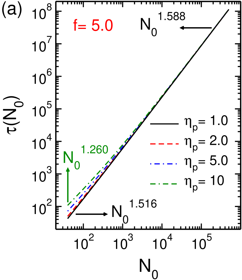
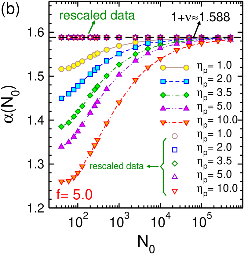
The dependence on the pore friction is even more clear in Fig. ​3 ​(b), where we have plotted the effective translocation exponent defined as $\alpha(N_{0})=\textrm{d}\ln\tau/(\textrm{d}\ln N_{0})$ ikonen2013 for different values of pore friction. We have checked the chain length dependence of the translocation exponent for the specific case of fixed pore friction $\eta_{\textrm{p}}=3.5$, when the thermal fluctuations as well as distribution of the initial configurations of the chain are taken into account. For both cases the translocation exponents are the same as of the deterministic case within a quite good accuracy. As mentioned, the dependence of the translocation exponents on the pore friction is more pronounced for short chain lengths. To show that the difference from the asymptotic value is indeed caused by the pore friction term, and not some other finite size effects, we define a rescaled translocation time as

$$\tilde{\tau}^{{\dagger}}=\tilde{\tau}-c_{2}\tilde{\eta}_{\textrm{p}}N_{0}=c_{1}N_{0}^{1+\nu}\sim N_{0}^{\alpha^{{\dagger}}},$$ (12)

where $\alpha^{{\dagger}}\equiv 1+\nu$ is the rescaled translocation exponent which does not depend on the chain length. As explained in Ref. ikonen2013 , $c_{1}$ and $c_{2}$ can be obtained by calculating the intercept and slope of the curve $\tau/N_{0}^{1+\nu}$ as a function of $\tilde{\eta}_{\textrm{p}}N_{0}^{-\nu}$, respectively. Calculating the rescaled exponent as $\alpha^{{\dagger}}(N_{0})=\textrm{d}\ln\tau^{{\dagger}}/(\textrm{d}\ln N_{0})$ it is found that it is indeed equal to $1+\nu$ for all chain lengths, independent of pore friction which is demonstrated in Fig. ​3 ​(b). This result is in excellent agreement with the molecular dynamics simulation results discussed in Ref. ikonen2013 .

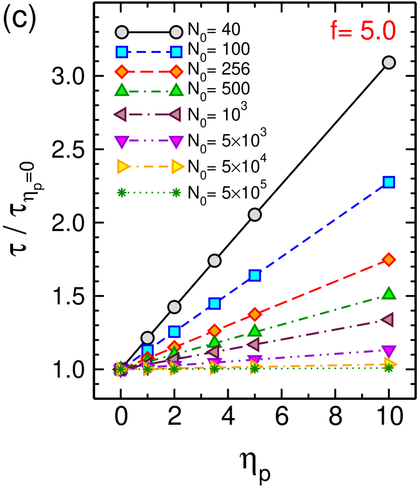
To further illustrate the influence of the pore friction on the translocation time, in Fig. ​3 ​(c) the normalized translocation time, $\tau/\tau_{\eta_{\textrm{p}}=0}$, has been plotted as a function of the pore friction, $\eta_{\textrm{p}}$, for various values of chain length, $N_{0}=40-5\times 10^{5}$. As it can be seen the normalized translocation time is influenced strongly by the pore friction for shorter chains while for longest chain the translocation time is constant for different values of the pore friction.

V.2 Waiting time distribution

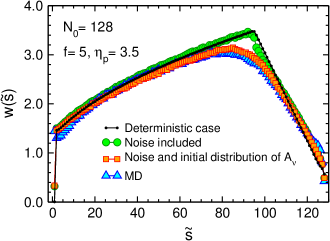
An important quantity in examining the dynamics of the translocation process is the monomer waiting time, which is defined as the time that each monomer or segment spends at the pore during the translocation process. The waiting time is calculated for each monomer, and averaged over the different simulation trajectories. Here we have calculated the waiting time as a function of the translocation coordinate $\tilde{s}$ and present it in Fig. ​4 for a fixed chain length $N_{0}=128$, external driving force $f=5.0$ and $\eta_{\textrm{p}}=3.5$. It can be seen that the translocation process is a far-from-equilibrium process and has two different stages. First one is the propagation stage where as the time passes more monomers are moved and involved in the drag friction force. Therefore the friction increases monotonically until it gets its maximum value which happens when the tension reaches the chain end. The second stage of the translocation process is called the post propagation stage that starts when the tension reaches the chain end. During this stage the remaining part of the chain in the cis side is sucked through the pore and at the end the translocation process ends when the whole chain passes through the pore to the trans side.

We can now use the IFTP model to separately examine the influence of thermal fluctuations in the noise and the distribution of the initial configuration of the chain. The results are shown in Fig. ​4. The black curve corresponds to the deterministic case, where both the force $f=5.0$ and the amplitude $A_{\nu}=1.15$ are fixed. The green circles show the waiting time when the force includes the stochastic component (noise) $\zeta$ and $A_{\nu}=1.15$ is fixed. As can be seen, the mean values are almost identical to the first deterministic case. The red squares exhibit the waiting time when both the force and $A_{\nu}$ are stochastic, i.e. the force includes noise and the initial distribution of $A_{\nu}$ is sampled from Eq. ​(10). The main effect of the stochastic sampling of the initial configurations is to smoothen the transition from the propagation to the post-propagation stage. This is a feature that is also seen in molecular dynamics simulations (blue triangles), where the initial configuration is sampled by thermalizing the polymer before each simulation trajectory. All in all, there is now a very good agreement between the theory and the MD simulations.

Figure 4: Waiting time, $w(\tilde{s})$, as a function of the translocation coordinate, $\tilde{s}$. Here, we present waiting time for different cases when both of the force and $A_{\nu}=1.15$ are deterministic (black curve), force is chosen randomly but $A_{\nu}=1.15$ is deterministic (green circles), both the force and $A_{\nu}$ are stochastic (red squares), and finally MD simulation data (blue triangles).

V.3 Distribution of translocation time

Another quantity which is of fundamental interest is the translocation time distribution which is depicted in Fig. ​5. The green bars present the histogram of the translocation time for fixed $A_{\nu}=1.15$ (noise included). Here the distribution is solely due to the randomness of the driving force. The red bars show the histogram where $A_{\nu}(y)$ has been sampled using Eq. ​(10) as $A_{\nu}(y)=yA_{\nu}$ where $A_{\nu}=1.15$ (noise and initial distribution of $A_{\nu}$). To compare the results of the theoretical model with MD data, the histogram of the translocation times based on MD simulations is also shown as blue bars. As it can be seen, the distribution with fixed $A_{\nu}$ is much narrower than the MD result. This is in agreement with the observations of Ref. ikonen2012a . However, there is a much better agreement with MD when the initial configurations are randomly sampled. Here the distribution gets wider and agrees quite well with the MD data, in particular for long translocation times. However, the model predicts slightly faster translocation events than the MD. The reason for this is easy to understand. In choosing the prefactor $A_{\nu}$ as the parameter describing the variance in the initial configurations, we ensure that the end-to-end distance distribution is well reproduced. However, the shape of the chain remains unchanged. Specifically, the form $\tilde{R}\propto N_{0}^{\nu}$ excludes configurations where the chain extends far away from the pore but loops back so that the end-to-end distance becomes small. Thus the drag due to the long loops is not entirely accounted for, and the effective friction and consequently the translocation time are underestimated. This result also indicates that it may be necessary to express the equilibrium shape of the chain with more than just one parameter to capture the variation in the translocation time in detail.

Figure 5: The translocation time histogram as a function of translocation time $\tau$. The green bars present the normalized histogram when $A_{\nu}=1.15$ is deterministic while the external driving force is $f=5.0$ and the total force includes the stochastic contribution. The red bars correspond to solutions where $A_{\nu}(y)$ is also chosen from Eq. ​(10). The histogram of the translocation time based on MD simulation is illustrated by blue bars.

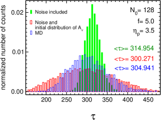
V.4 Evolution of the translocation coordinate $\tilde{s}$ as a function of time

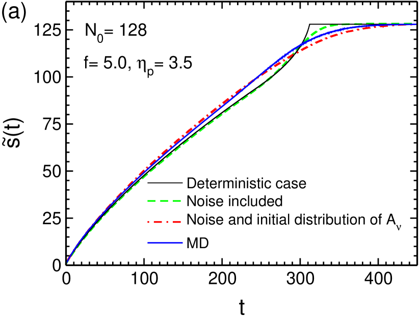
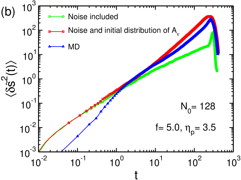
Finally, we examine how the translocation coordinate and its fluctuations evolve in time. These quantities could not be explained with the previous BDTP theory of Refs. ikonen2012a ; ikonen2012b . Here we have again chosen the chain length $N_{0}=128$, driving force $f=5.0$ and the pore friction as $\eta_{\textrm{p}}=3.5$. The results for $\tilde{s}(t)$ can be seen in Fig. ​6 ​(a), and for the variance $\langle\delta\tilde{s}^{2}(t)\rangle\equiv\langle\tilde{s}^{2}(t)\rangle-\langle\tilde{s}(t)\rangle^{2}$ in Fig. ​6 ​(b). We have again solved the model with the stochastic force term first off and with fixed initial configuration (black curve), then with thermal noise included in the force (green curves), and both thermal noise and randomly sampled initial configurations (red curves). We also compare the results with MD, shown with blue curves.

The fully deterministic solution (the black $\tilde{s}(t)$ curve) is quite different from the MD solution towards the end, and approaches the final value of $\tilde{s}=128$ much more sharply. The shape is very similar to that shown in, e.g., Refs. sakaue2010 ; dubbeldam2014 . Adding the fluctuations to the driving force makes the approach to the terminal value a bit smoother. However, the larger difference comes again from the initial configurations. With the random selection of the end-to-end distance, the results match very well with MD data.

For the fluctuations of $\tilde{s}$, the results are similar. With just the thermal fluctuations in the driving force, the variance increases much slower than the MD results. This is consistent with the earlier study of Ref. ikonen2012b . When the initial configuration is randomized, the results are much improved and are again in good agreement with MD. However, similar to the distribution of the translocation time discussed above, the magnitude of the fluctuations is slightly overestimated.

Figure 6: (a) The translocation coordinate, $\tilde{s}(t)$, as a function of time, $t$, when both the force and $A_{\nu}$ are deterministic (black solid line), force includes noise but $A_{\nu}$ is deterministic (green dashed line), both force and $A_{\nu}$ are stochastic (red dashed-dotted line), and the MD data (blue line). (b) The fluctuations of the translocation coordinate, $\langle\delta\tilde{s}^{2}(t)\rangle\equiv\langle\tilde{s}^{2}(t)\rangle-\langle\tilde{s}(t)\rangle^{2}$, as a function of time for the cases when the force includes noise while $A_{\nu}$ is deterministic (green), both force and $A_{\nu}$ are stochastic (red), and for MD simulations (blue). Here, we have chosen fixed chain length $N_{0}=128$, external driving force $f~{}\!=~{}\!5.0$ and the pore friction as $\eta_{\textrm{p}}=3.5$.

VI Conclusions

In this paper we have derived a model of driven polymer translocation based on combined Brownian dynamics-tension propagation theory in the constant flux approximation. The model gives an explicit equation of motion for the position of the tension front and allows a full characterization of the translocation process. In particular, it can be used to derive a finite-size formula for the scaling of the translocation time as a function of the chain length, revealing that the main correction-to-scaling term comes from the pore friction and is linearly proportional to $N_{0}$. The model reproduces the chain length dependence of the effective scaling exponents from the previous BDTP theory ikonen2012a ; ikonen2012b ; ikonen2013 . Moreover, it allows a detailed study of the interplay between thermal noise in the force and initial distribution of the chain configurations. The analysis presented here shows that by including the latter effect, quantities such as the waiting time, the distribution of translocation time and the dynamics and fluctuations in the translocation coordinate are in good agreement with the MD data. This reveals the important role of the cis side of the chain to driven translocation and justifies the approximation to neglect the trans side degrees of freedom from the model.

Appendix A Force at distance $\tilde{x}$ to the pore

The value of the force as a function of the distance to the pore, $\tilde{x}$, on the cis side can be obtained for the trumpet regime by integrating the force balance relation, $d\tilde{f}(\tilde{x}^{\prime})=-\tilde{\phi}(\tilde{t})~{}d~{}\!\!\tilde{x}^{\prime}$, for a differential element $d\tilde{x}^{\prime}$ over the distance between 0 and $\tilde{x}$ as

$$\tilde{f}(\tilde{x})=\tilde{f}_{0}-\tilde{\phi}(\tilde{t})\tilde{x},$$ (13)

where $\tilde{f}_{0}$ is the force at the entrance of the pore. Note that here we have used the iso-flux assumption which means that the value of the monomer flux, $\tilde{\phi}$, is constant over the integration range $[0,\tilde{x}]$.

In the stem-flower regime, the region of mobile beads is separated into two sub-regions. In the stem region the chain is straightened because the tension force is stronger and in the flower region as the tension force is weaker, blobs are formed. The border between the stem and the flower regions is at $\tilde{x}=\tilde{r}(\tilde{t})$ where the tension force has the value of unity. Writing the force balance equation for a differential element and integrating over the stem region, $\tilde{r}(\tilde{t})$ can be found as

$$\tilde{r}(\tilde{t})=\frac{\tilde{f}_{0}-1}{\tilde{\phi}(\tilde{t})}.$$ (14)

Then by integrating the force balance equation over the distance between $\tilde{r}$ and $\tilde{x}$, that $\tilde{f}(\tilde{r})=1$, in the flower regime one can write the following relation

$$\tilde{f}(\tilde{x})=1-\tilde{\phi}(\tilde{t})~{}\!(\tilde{x}-\tilde{r}).$$ (15)

Combining Eqs. ​(14) and (15) the same relation similar to the trumpet regime can be obtained for the stem-flower regime as $\tilde{f}(\tilde{x})=\tilde{f}_{0}-\tilde{\phi}(\tilde{t})\tilde{x}$.

Appendix B Equation of motion for the tension front

To find an equation for the time evolution of the tension front location, $\tilde{R}$, for the propagation stage one must calculate and then substitute $\tilde{l}$, the number of mobile beads on the cis side, and $\tilde{s}$ into the closure relation

$$\tilde{R}=A_{\nu}[\tilde{l}+\tilde{s}]^{\nu},$$ (16)

and then perform the time derivative of $\tilde{R}$ that can be read as a function of $\dot{\tilde{l}}(\tilde{t})$ and $\dot{\tilde{s}}(\tilde{t})$ as

$$\dot{\tilde{R}}(\tilde{t})=\nu A_{\nu}^{1/\nu}\tilde{R}(\tilde{t})^{\frac{\nu-1}{\nu}}[\dot{\tilde{l}}(\tilde{t})+\dot{\tilde{s}}(\tilde{t})],$$ (17)

where by definition

$$\frac{d\tilde{s}(\tilde{t})}{d\tilde{t}}=\dot{\tilde{s}}(\tilde{t})=\tilde{\phi}(\tilde{t}).$$ (18)

The number of mobile monomers in the cis side, i.e. $\tilde{l}(\tilde{t})$, is obtained by integrating the linear monomer number density, $\tilde{\sigma}(\tilde{t})$, over the distance between $0$ and $\tilde{R}$. Therefore, first the monomer number density must be obtained. To this end the blob theory can be used. When a blob is constructed by applying the tension force on the backbone of the chain, the blob size, $\tilde{\xi}(\tilde{x})$, can be obtained as $\tilde{\xi}(\tilde{x})=1/|\tilde{f}(\tilde{x})|$ where $\tilde{f}(\tilde{x})=\tilde{f}_{0}-\tilde{\phi}(\tilde{t})\tilde{x}$ is the force at the distance $\tilde{x}$ to the pore in the cis side which has been obtained in Appendix A. On length scales shorter than the Pincus blob size, $\tilde{\xi}(\tilde{x})$, the chain behaves as if undisturbed by the external driving force and the blob size scales as $\tilde{\xi}=g^{\nu}$, where $g$ is the number of monomers inside the blob. Finally the monomer number density is given by $\tilde{\sigma}(\tilde{x},\tilde{t})=\frac{g}{\tilde{\xi}}=\tilde{\xi}^{\frac{1}{\nu}-1}=\big{|}\tilde{f}(\tilde{x})\big{|}^{1-\frac{1}{\nu}}$. Using the above monomer number density the number of mobile monomers in the cis side can be derived as

$$\tilde{l}(\tilde{t})=\int_{0}^{\tilde{R}(\tilde{T})}\tilde{\sigma}(\tilde{x},\tilde{t})d\tilde{x}.$$ (19)

Therefore, for the trumpet regime

$$\tilde{l}_{\textrm{T}}(\tilde{t}) = \int_{0}^{\tilde{R}(\tilde{t})}\tilde{\sigma}(\tilde{x},\tilde{t})d\tilde{x}=\int_{0}^{\tilde{R}(\tilde{t})}|\tilde{f}(\tilde{x})|^{(\nu-1)/\nu}d\tilde{x}=$$ (20)

$$= \int_{0}^{\tilde{R}(\tilde{t})}\big{|}\tilde{f}_{0}-\tilde{\phi}(\tilde{t})\tilde{x}\big{|}^{(\nu-1)/\nu}d\tilde{x}$$

$$= \int_{0}^{\tilde{R}(\tilde{t})}\bigg{|}\tilde{\phi}(\tilde{t})\tilde{R}(\tilde{t})-\tilde{\phi}(\tilde{t})\tilde{x}\bigg{|}^{(\nu-1)/\nu}d\tilde{x}.$$

Consequently

$$\tilde{l}_{\textrm{T}_{+}}(\tilde{t}) =\frac{\nu}{(2\nu-1)}\tilde{\phi}(\tilde{t})^{\frac{\nu-1}{\nu}}\tilde{R}(\tilde{t})^{\frac{2\nu-1}{\nu}}~{}~{}~{}:\tilde{\phi}(\tilde{t})>0,$$ (21a)

$$\tilde{l}_{\textrm{T}_{-}}(\tilde{t}) =\frac{\nu}{(2\nu-1)}[-\tilde{\phi}(\tilde{t})]^{\frac{\nu-1}{\nu}}\tilde{R}(\tilde{t})^{\frac{2\nu-1}{\nu}}\!:\tilde{\phi}(\tilde{t})<0,$$ (21b)

where the subscript T denotes the trumpet regime, and $+$ and $-$ stand for the positive and negative values of $\tilde{\phi}(\tilde{t})$, respectively.

To obtain $\tilde{l}_{\textrm{SF}}(\tilde{t})$, which is the number of mobile monomers in the cis side in the stem-flower regime, similar to the procedure for the trumpet regime, one has to integrate the linear monomer number density, $\tilde{\sigma}(\tilde{t})$, over the distance from 0 to $\tilde{R}$, i.e.

$$\tilde{l}_{\textrm{SF}}(\tilde{t}) = \int_{0}^{\tilde{R}(\tilde{t})}\tilde{\sigma}(\tilde{x},\tilde{t})d\tilde{x}$$ (22)

$$= \int_{0}^{\tilde{r}(\tilde{t})}\tilde{\sigma}(\tilde{x},\tilde{t})d\tilde{x}+\int_{\tilde{r}(\tilde{t})}^{\tilde{R}(\tilde{t})}\tilde{\sigma}(\tilde{x},\tilde{t})d\tilde{x}$$

$$= \tilde{r}(\tilde{t})+\int_{\tilde{r}(\tilde{t})}^{\tilde{R}(\tilde{t})}|\tilde{f}(\tilde{x})|^{(\nu-1)/\nu}d\tilde{x}$$

$$= \frac{\tilde{\phi}(\tilde{t})\tilde{R}(\tilde{t})-1}{\tilde{\phi}(\tilde{t})}$$

$$+\int_{\tilde{r}(\tilde{t})}^{\tilde{R}(\tilde{t})}\bigg{|}\tilde{\phi}(\tilde{t})\tilde{R}(\tilde{t})-\tilde{\phi}(\tilde{t})\tilde{x}\bigg{|}^{(\nu-1)/\nu}d\tilde{x}.$$

Performing the integral yields $\tilde{l}_{\textrm{SF}}(\tilde{t})$ as

$$\tilde{l}_{\textrm{SF}}(\tilde{t})=\tilde{R}(\tilde{t})+\frac{1-\nu}{(2\nu-1)}\frac{1}{\tilde{\phi}(\tilde{t})},$$ (23)

where the index SF denotes the stem-flower regime. Then the time derivative of the number of mobile beads, $\dot{\tilde{l}}(\tilde{t})$ can be cast into

$$\dot{\tilde{l}}_{\textrm{a}}(\tilde{t})={\cal{L}}_{\textrm{a}}\times[\dot{\tilde{f}}_{\textrm{tot}}(\tilde{t})-\tilde{\phi}(\tilde{t})\dot{\tilde{R}}(\tilde{t})]+\tilde{{\cal{G}}}_{\textrm{a}}\times\dot{\tilde{f}}_{\textrm{tot}}(\tilde{t}),$$ (24)

where ${\textrm{a}}={\textrm{T}_{+}},~{}{\textrm{T}_{-}}~{}{\textrm{and}}~{}{\textrm{SF}}$, and

$${\cal{L}}_{\textrm{T}_{+}} =\frac{1}{\tilde{\eta}_{\textrm{p}}+\tilde{R}(\tilde{t})}\bigg{\{}-\frac{\nu}{(2\nu-1)\tilde{\phi}(\tilde{t})^{2}}\big{[}\tilde{\phi}(\tilde{t})\tilde{R}(\tilde{t})\big{]}^{\frac{2\nu-1}{\nu}}$$

$$-\frac{\tilde{\eta}_{\textrm{p}}}{\tilde{\phi}(\tilde{t})}\big{[}\tilde{\phi}(\tilde{t})\tilde{R}(\tilde{t})\big{]}^{\frac{\nu-1}{\nu}}\bigg{\}},\hskip 42.67912pt:~{}\tilde{\phi}(\tilde{t})>0$$ (25a)

$${\cal{L}}_{\textrm{T}_{-}} =\frac{1}{\tilde{\eta}_{\textrm{p}}+\tilde{R}(\tilde{t})}\bigg{\{}\frac{\nu}{(2\nu-1)\tilde{\phi}(\tilde{t})^{2}}\big{[}-\tilde{\phi}(\tilde{t})\tilde{R}(\tilde{t})\big{]}^{\frac{2\nu-1}{\nu}}$$

$$-\frac{\tilde{\eta}_{\textrm{p}}}{\tilde{\phi}(\tilde{t})}\big{[}-\tilde{\phi}(\tilde{t})\tilde{R}(\tilde{t})\big{]}^{\frac{\nu-1}{\nu}}\bigg{\}},\hskip 28.45274pt:~{}\tilde{\phi}(\tilde{t})<0$$ (25b)

$$\tilde{{\cal{G}}}_{\textrm{T}_{+}} =\frac{1}{\tilde{\phi}(\tilde{t})}\big{[}\tilde{\phi}(\tilde{t})\tilde{R}(\tilde{t})\big{]}^{\frac{\nu-1}{\nu}}\hskip 51.21504pt:~{}\tilde{\phi}(\tilde{t})>0,$$ (25c)

$$\tilde{{\cal{G}}}_{\textrm{T}_{-}} =\frac{1}{\tilde{\phi}(\tilde{t})}\big{[}-\tilde{\phi}(\tilde{t})\tilde{R}(\tilde{t})\big{]}^{\frac{\nu-1}{\nu}}\hskip 39.83368pt:~{}\tilde{\phi}(\tilde{t})<0,$$ (25d)

$${\cal{L}}_{\textrm{SF}} =\frac{1}{\tilde{\eta}_{\textrm{p}}+\tilde{R}(\tilde{t})}\bigg{[}-\frac{\tilde{\eta}_{\textrm{p}}\tilde{\phi}(\tilde{t})+\tilde{\phi}(\tilde{t})\tilde{R}(\tilde{t})}{\tilde{\phi}(\tilde{t})^{2}}$$

$$+\frac{\nu-1}{(2\nu-1)\tilde{\phi}(\tilde{t})^{2}}\bigg{]},$$ (25e)

$${\cal{G}}_{\textrm{SF}} =\frac{1}{\tilde{\phi}(\tilde{t})}.$$ (25f)

Combining Eqs. (17), (18) and (24) the equation for the time evolution of the tension front can be written as

$$\dot{\tilde{R}}(\tilde{t})=\frac{\nu A_{\nu}^{\frac{1}{\nu}}\tilde{R}(\tilde{t})^{\frac{\nu-1}{\nu}}\big{[}({\cal{L}}_{\textrm{a}}+{\cal{G}}_{\textrm{a}})\times\dot{\tilde{f}}_{\textrm{tot}}(\tilde{t})+\tilde{\phi}(\tilde{t})\big{]}}{1+\nu A_{\nu}^{\frac{1}{\nu}}\tilde{R}(\tilde{t})^{\frac{\nu-1}{\nu}}{\cal{L}}_{\textrm{a}}\times\tilde{\phi}(\tilde{t})}.$$ (26)

In the post propagation stage, the closure relation is given by the sum over the number of mobile beads in the cis side, $\tilde{l}$, and the number of translocated beads, $\tilde{s}$, as $\tilde{l}+\tilde{s}=N_{0}$. The time derivative of this closure relation is

$$\dot{\tilde{l}}+\dot{\tilde{s}}=0.$$ (27)

Combining Eqs. ​(18), (24) and (27) the equation of motion for the tension front in the post propagation stage can be cast into:

$$\dot{\tilde{R}}(\tilde{t})=\frac{({\cal{L}}_{\textrm{a}}+{\cal{G}}_{\textrm{a}})\dot{\tilde{f}}_{\textrm{tot}}(\tilde{t})+\tilde{\phi}(\tilde{t})}{\tilde{\phi}(\tilde{t})\times{\cal{L}}_{\textrm{a}}}.$$ (28)

References

- (1) J.J. Kasianowicz, E. Brandin, D. Branton and D.W. Deamer, Proc. Natl. Acad. Sci. 93, 13770 (1996).
- (2) A. Meller, J. Phys. Condens. Matter 15, R581 (2003).
- (3) M. Muthukumar, Polymer Translocation (Taylor and Francis, 2011).
- (4) A. Milchev, J. Phys.: Condens. Matter 23, 103101 (2011).
- (5) V. V. Palyulin, T. Ala-Nissila and R. Metzler, Soft Matter, 2014, DOI: 10.1039/C4SM01819B.
- (6) E.E. Schadt, S. Turner and A. Kasarskis, Hum Mol Gen 19, R227 (2010).
- (7) D. Branton, D.W. Deamer, A. Marziali et al., Nature Biotech. 26, 1146 (2008).
- (8) A.J. Storm et al, Nano Lett. 5, 1193 (2005).
- (9) W. Sung and P.J. Park, Phys. Rev. Lett. 77, 783 (1996).
- (10) M. Muthukumar, J. Chem. Phys. 111, 10371 (1999).
- (11) J. Chuang, Y. Kantor and M. Kardar, Phys. Rev. E 65, 011802 (2001).
- (12) R. Metzler and J. Klafter, Biophys. J. 85, 2776 (2003).
- (13) Y. Kantor and M. Kardar, Phys. Rev. E 69, 021806 (2004).
- (14) K. Luo, S.T.T. Ollila, I. Huopaniemi, T. Ala-Nissila, P. Pomorski, M. Karttunen, S.-C. Ying and A. Bhattacharya, Phys. Rev. E 78 050901(R) (2008).
- (15) K. Luo, T. Ala-Nissila, S.-C. Ying and R. Metzler, Europhys. Lett. 88, 68006 (2009).
- (16) J.L.A. Dubbeldam, A. Milchev, V.G. Rostiashvili and T.A. Vilgis, Europhysics Lett. 79, 18002 (2007).
- (17) A. Yu. Grosberg, S. Nechaev, M. Tamm and O. Vasilyev, Phys. Rev. Lett. 96, 228105 (2006).
- (18) T. Sakaue, Phys. Rev. E 76, 021803 (2007).
- (19) T. Sakaue, in Proceedings of the 5th Workshop on Complex Systems, AIP CP, Vol. 982, p. 508 (2008).
- (20) T. Sakaue, Phys. Rev. E 81, 041808 (2010).
- (21) T. Saito and T. Sakaue, Eur. Phys. J. E 34, 135 (2012).
- (22) T. Saito and T. Sakaue, Phys. Rev. E 85, 061803 (2012).
- (23) T. Saito and T. Sakaue, arXiv:1205.3861 (2012).
- (24) P. Rowghanian and A. Y. Grosberg, J. Phys. Chem. B 115, 14127 (2011).
- (25) J. L. A. Dubbeldam, V. G. Rostiashvili, A. Milchev and T. A. Vilgis, Phys. Rev. E 85, 041801 (2012).
- (26) T. Ikonen, A. Bhattacharya, T. Ala-Nissila and W. Sung, Phys. Rev. E 85, 051803 (2012).
- (27) T. Ikonen, A. Bhattacharya, T. Ala-Nissila and W. Sung, J. Chem. Phys. 137, 085101 (2012).
- (28) T. Ikonen, A. Bhattacharya, T. Ala-Nissila, W. Sung, Europhys. Lett 103, 38001 (2013).
- (29) V. Lehtola, R.P. Linna and K. Kaski, Europhys. Lett. 85, 58006 (2009).
- (30) A. Bhattacharya, W.H. Morrison, K. Luo, T. Ala-Nissila, S.-C. Ying, A. Milchev and K. Binder, Eur. Phys. J. E 29, 423 (2009).
- (31) V.V. Lehtola, K. Kaski, R.P. Linna, Phys. Rev. E 82, 031908 (2010).
- (32) A. Bhattacharya and K. Binder, Phys. Rev. E 81, 041804 (2010).
- (33) H. W. de Haan and G. W. Slater, Phys. Rev. E 81, 051802 (2010).
- (34) H. W. de Haan and G. W. Slater, J. Chem. Phys. 136, 204902 (2012).
- (35) M. G. Gauthier and G. W. Slater, Phys. Rev. E 79, 021802 (2009).
- (36) J. M. Polson and A. C. M. McCaffrey, J. Chem. Phys. 138, 174902 (2013).
- (37) P. M. Suhonen, K. Kaski and R. Linna, arXiv:1405.0920 (2014).
- (38) J. L. A. Dubbeldam, V. G. Rostiashvili and T. A. Vilgis, arXiv:1404:0167 (2014).
- (39) E. A. DiMarzio, C. M. Guttman and J. D. Hoffman, Faraday Discuss. Chem. Soc. 68, 210 (1979).