Current-induced spin torque resonance of magnetic insulators affected by field-like spin-orbit torques and out-of-plane magnetizations

Abstract

The spin-torque ferromagnetic resonance (ST-FMR) in a bilayer system consisting of a magnetic insulator such as $\mathrm{Y_{3}Fe_{5}O_{12}}$ and a normal metal with spin-orbit interaction such as Pt is addressed theoretically. We model the ST-FMR for all magnetization directions and in the presence of field-like spin-orbit torques based on the drift-diffusion spin model and quantum mechanical boundary conditions. ST-FMR experiments may expose crucial information about the spin-orbit coupling between currents and magnetization in the bilayers.

I Introduction

Near-dissipationless propagation of spin waves utilizing magnetic insulators such as $\mathrm{Y_{3}Fe_{5}O_{12}}$ (YIG) with very low magnetization damping by Pt contacts creates an interface between spinelectronic and magnonic circuits for low power data transmission.Kajiwara ; Wu However, the interpretation of experiments of current-induced coherent spin waves or magnetization dynamics is unclear by the strongly non-linear proses with a problematic threshold.Xiao Spin wave mediated transport in YIG$|$Pt bilayer has only recently been discovered and attracted a great deal of interest since it revealed new physics by, e.g., the spin Seebeck effect (SSE)Uchida10 and spin Hall magnetoresistance (SMR), Nakayama ; Chen implying application potential for low-dissipation spintronic interconnects and large area thermoelectric power generation. The SMR refers to the dependence of the electrical resistance of the normal metal on the magnetization angle of an adjacent magnetic insulator and is caused by a simultaneous operation of the Spin Hall Effect (SHE) review12 and its inverse (ISHE) as a nonequilibrium proximity phenomenon. Many experiments have been described quantitatively well by the SMR model with one set of parameters.Althammer ; Hahn ; Vlietstra ; Marmion ; Lin ; Isasa The magnetoresistance enables straightforward access to the effects of spin-orbit coupling between currents and magnetization in the bilayers.

The spin current through a ferromagnet$|$normal metal interface is governed by the complex spin-mixing conductance (per unit area of the interface) $G^{\uparrow\downarrow}=G_{r}+iG_{i}$. Tserkovnyak05 The prediction of a large $G_{r}$ for interfaces between YIG and simple metals by first-principle calculations Jia11 has been amply confirmed by recent experiments.Weiler The imaginary part $G_{i}$ can be interpreted as an effective exchange field between magnetization and spin accumulation, which in the absence of spin-orbit interaction is usually much smaller than the real part. However, in metallic structures field-like spin-orbit torques (SOTs) have been found, which can be modelled by a significant $G_{i}$.Pai14 ; Kim14 Current-induced SOTs are often associated with the Rashba spin-orbit interaction.Haney ; Skinner In the absence of evidence for large SOTs in bilayers with magnetic insulators we disregarded $G_{i}$ in our previous work.Chiba14 However, there is no evidence against a strong spin-orbit interaction at YIG$|$Pt interfaces either. The SMR phenomenology, for example, can be also explained by an interface Rashba interaction.Grigoryan14

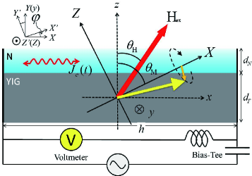
Figure 1: Schematic set-up to observe the SMR rectified voltage in which $\mathbf{H_{\mathrm{ex}}}$ is an external magnetic field and $\theta_{\mathrm{H}}$ and $\theta_{\mathrm{M}}$ show the external magnetic field and the magnetization angles. The YIG($d_{F}$ nm)$|$N($d_{N}$ nm) bilayer film is patterned into a strip with a length $h$. A Bias-Tee allows detection of a dc voltage under an ac bias.

In bilayer thin films made from a ferromagnetic and a normal metal, a dc voltage is generated from the magnetization dynamics induced by an applied ac spin-transfer torque and the anisotropic magnetoresistance (AMR). This current-induced spin torque ferromagnetic resonance (ST-FMR) is an established noninvasive method to study the spin-orbit coupling between currents and magnetization.Liu The spin-orbit coupling between currents and magnetization in the YIG$|$Pt system can also be accessed in this manner by utilizing the SMR as shown in Fig. 1.Chiba14

Here we generalize our previous work on ST-FMR for bilayers of a ferro- or ferrimagnetic insulator (FI) and a heavy normal metal (N)Chiba14 by deriving magnetization dynamics and dc voltages for arbitrary equilibrium magnetization directions and include heuristically a possibly large field-like SOT in terms of a significant imaginary part of the spin-mixing conductance.

II Magnetization dynamics with spin-orbit torques

The ac current with frequency $\omega_{a}=2\pi f_{a}$ induces a spin accumulation distribution $\boldsymbol{\mu}_{s}(z,t)$ in N that fills the spin-diffusion equation

$$\partial_{t}\boldsymbol{\mu}_{s}=D\partial_{z}^{2}\boldsymbol{\mu}_{s}-\frac{\boldsymbol{\mu}_{s}}{\tau_{\mathrm{sf}}},$$ (1)

where $D$ is the charge diffusion constant and $\tau_{\mathrm{sf}}$ spin-flip relaxation time in N with the spin-diffusion length $\lambda=\sqrt{D\tau_{\mathrm{sf}}}$. The ISHE induces a charge current in the $x$-$y$ plane by the diffusion spin current along the $z$-direction, $\overline{J_{c,x}}(t)$=$J_{\mathrm{SMR}}(t)+J_{\mathrm{SP}}(t)$ which is averaged over the N film thickness $d_{N}$, where $J_{\mathrm{SMR}}(t)$ and $J_{\mathrm{SP}}(t)$ are SMR rectification and spin pumping-induced charge currents with $J_{c}^{0}(t)=J_{c}^{0}\operatorname{Re}(e^{i\omega_{a}t})$.Chiba14

ST-FMR experiments utilize the ac impedance of the oscillating transverse spin Hall current caused by the induced magnetization dynamics that is described by the Landau-Lifshitz-Gilbert (LLG) equation including the interface spin current $\boldsymbol{J}_{s}^{F|N}=\boldsymbol{J}_{s}^{T}+\boldsymbol{J}_{s}^{P}$ with

$$\boldsymbol{J}_{s}^{T} =\frac{G_{r}}{e}\hat{\mathbf{M}}\times\left(\hat{\mathbf{M}}\times\boldsymbol{\mu}_{s}^{F|N}\right)+\frac{G_{i}}{e}\hat{\mathbf{M}}\times\boldsymbol{\mu}_{s}^{F|N},$$ (2)

$$\boldsymbol{J}_{s}^{P} =\frac{\hbar}{e}\left(G_{r}\hat{\mathbf{M}}\times\partial_{t}\hat{\mathbf{M}}+G_{i}\partial_{t}\hat{\mathbf{M}}\right),$$ (3)

as the additional torques $\boldsymbol{\tau}_{J}=\gamma\hbar\boldsymbol{J}_{s}^{F|N}/(2eM_{s}d_{F})$ $(e=-|e|)$, where $\boldsymbol{\mu}_{s}^{F|N}$, $\hat{\mathbf{M}}$, $\gamma$, $M_{s}$, and $d_{F}$ are the interface spin accumulation between FI and N layers, the unit vector along the FI magnetization, the gyromagnetic ratio, the saturation magnetization, and the thickness of the FI film, respectively. The external magnetic field $\mathbf{H_{\mathrm{ex}}}$ is applied at a polar angle $\theta_{\mathrm{H}}$, especially in the $z$-$x$ plane corresponding to the angle $\alpha$ in Ref. Bai13, , and azimuth $\varphi$ in the $x$-$y$ plane. It is convenient to consider the magnetization dynamics in the $(\theta_{\mathrm{M}}-\pi/2)$ around the $y$-axis and $\varphi$ around the $Z$-axis rotated coordinate system [see Fig. 1]. Denoting the transformation matrix as $R(\theta_{\mathrm{M}}-\pi/2,\varphi)$, the magnetization dynamics $\mathbf{M}_{R}(t)=R(\theta_{\mathrm{M}}-\pi/2,\varphi)\mathbf{M}(t)$ precessing around the $Z^{\prime}$-axis obeys the LLG equation in the $X^{\prime}Y^{\prime}Z^{\prime}$-coordinate system (Fig. 1),

$$\partial_{t}\hat{\mathbf{M}}_{R}=-\tilde{\gamma}\hat{\mathbf{M}}_{R}\times\left(\mathbf{H}_{\mathrm{eff},R}+\mathbf{H}_{J,R}\right)+\alpha\hat{\mathbf{M}}_{R}\times\partial_{t}\hat{\mathbf{M}}_{R},$$ (4)

where

$$\mathbf{H}_{\mathrm{eff},R} =\mathbf{H}_{\mathrm{ex}}+\mathbf{H}_{\mathrm{M}}+\mathbf{H}_{\mathrm{m}}(t)+\mathbf{H}_{\mathrm{ac}}(t)$$

$$=\begin{pmatrix}H_{\mathrm{ex}}\cos(\theta_{\mathrm{M}}-\theta_{\mathrm{H}})\\ 0\\ H_{\mathrm{ex}}\sin(\theta_{\mathrm{M}}-\theta_{\mathrm{H}})\end{pmatrix}-4\pi M_{s}\cos\theta_{\mathrm{M}}\begin{pmatrix}\cos\theta_{\mathrm{M}}\\ 0\\ \sin\theta_{\mathrm{M}}\end{pmatrix}$$

$$-4\pi m_{Z}(t)\sin\theta_{\mathrm{M}}\begin{pmatrix}\cos\theta_{\mathrm{M}}\\ 0\\ \sin\theta_{\mathrm{M}}\end{pmatrix}$$

$$+\begin{pmatrix}0\\ H_{ac}\cos\varphi\\ -H_{ac}\cos\theta_{\mathrm{M}}\sin\varphi\end{pmatrix}e^{i(\omega_{a}t+\delta)}$$ (5)

is, respectively, the sum of the external magnetic field, the static demagnetizing field, the dynamic demagnetization field, and the ac current-induced Oersted field. $\delta$ is the phase shift between Oersted field and current, which is governed by the details of the sample design and therefore treated as an adjustable parameter.Harder11 The current-induced effective field may be linearized

$$\mathbf{H}_{J,R} =(\hat{\mathbf{M}}_{R}\times H_{r}\hat{\mathbf{Y^{\prime}}}+H_{i}\hat{\mathbf{Y^{\prime}}})e^{i\omega_{a}t}$$

$$\approx\begin{pmatrix}0\\ H_{i}\cos\varphi+H_{r}\cos\theta_{\mathrm{M}}\sin\varphi\\ H_{r}\cos\varphi-H_{i}\cos\theta_{\mathrm{M}}\sin\varphi\end{pmatrix}e^{i\omega_{a}t},$$ (6)

$$H_{r(i)}=\frac{\hbar}{2|e|M_{s}d_{F}}\theta_{\mathrm{SH}}J_{c}^{0}\operatorname{Re}\left(\operatorname{Im}\right)\eta.$$ (7)

Here $\eta$ is the complex spin diffusion efficiency

$$\eta=\left(1-\frac{1}{\cosh(d_{N}/\lambda)}\right)\frac{\tilde{g}_{r}(1+\tilde{g}_{r})+\tilde{g}_{i}^{2}+i\tilde{g}_{i}}{(1+\tilde{g}_{r})^{2}+\tilde{g}_{i}^{2}}$$ (8)

with $\tilde{g}_{r(i)}=2\lambda\rho G_{r(i)}\coth(d_{N}/\lambda)$ and $\rho$, the resistivity of bulk N . It is plotted in Fig. 2 as a function of $r=d_{N}/\lambda$ and $g_{r(i)}=2\lambda\rho G_{r(i)}$.

$$\alpha=\frac{\alpha_{0}+\beta\coth(r/2)\operatorname{Re}\eta}{1-\beta\coth(r/2)\operatorname{Im}\eta}$$ (9)

is the modulated magnetization damping in terms of the Gilbert damping constant of the isolated film $\alpha_{0}$ and $\beta=\gamma\hbar^{2}/(4\lambda\rho e^{2}M_{s}d_{F})$, and $\tilde{\gamma}=\gamma/\left(1-\beta\coth(r/2)\operatorname{Im}\eta\right)$. The external magnetic field $\mathbf{H}_{\mathrm{ex}}$ is applied at a polar angle $\theta_{\mathrm{H}}$ in the $z$-$x$ plane as shown in Fig. 1. It is convenient to consider the magnetization dynamics in the $\theta_{\mathrm{M}}$ rotated coordinate system in which the magnetization is stabilized along the static equilibrium condition, $\mathbf{M}_{R}\times\mathbf{H}_{\mathrm{eff},R}=0$, obeys the relation between $\theta_{\mathrm{H}}$ and $\theta_{\mathrm{M}}$ as

$$H_{\mathrm{ex}}=2\pi M_{s}\sin 2\theta_{\mathrm{M}}/\sin(\theta_{\mathrm{M}}-\theta_{\mathrm{H}}).$$ (10)

The magnetization precesses around the static equilibrium condition $\mathbf{M}_{R}(t)=\mathbf{M}_{R}^{0}+\mathbf{m}_{R}(t)\approx\left(M_{s},m_{Y^{\prime}}(t),m_{Z^{\prime}}(t)\right)$, where $\mathbf{M}_{R}^{0}$ and $\mathbf{m}_{R}(t)$ are the static and dynamic components of the magnetization. For a small-angle precession around the equilibrium direction $\mathbf{M}_{R}^{0}$, $\mathbf{m}_{R}(t)=(0,\delta m_{Y^{\prime}}e^{i\omega_{a}t},\delta m_{Z^{\prime}}e^{i\omega_{a}t})$ $\left(\operatorname{Re}[\delta m_{Y^{\prime}}]\,\operatorname{Re}[\delta m_{Z^{\prime}}]\ll M_{s}\right)$, we linearize Eq. (4) and arrive at the FMR condition for the ac current frequencyAndo11

$$H_{\mathrm{FMR}}\cos(\theta_{\mathrm{M}}-\theta_{\mathrm{H}})=2\pi M_{s}\left(\cos 2\theta_{\mathrm{M}}+\cos^{2}\theta_{\mathrm{M}}\right)$$

$$+\sqrt{\left\{2\pi M_{s}\left(\cos 2\theta_{\mathrm{M}}-\cos^{2}\theta_{\mathrm{M}}\right)\right\}^{2}+(\omega_{a}/\tilde{\gamma})^{2}}.$$ (11)

The magnetization dynamics is

$$\begin{pmatrix}m_{Y^{\prime}}(t)\\ m_{Z^{\prime}}(t)\end{pmatrix} =\frac{1}{2\pi}\frac{e^{i\omega_{a}t}\Omega_{a}\cos\varphi}{\Omega_{\mathrm{H}}^{2}-\Omega_{a}^{2}+2i\tilde{\Delta}\Omega_{\mathrm{H}}}\begin{pmatrix}Y_{r}^{c}+iY_{i}^{c}\\ Z_{r}^{c}+iZ_{i}^{c}\end{pmatrix}$$

$$+\frac{1}{2\pi}\frac{e^{i\omega_{a}t}\Omega_{a}\cos\theta_{\mathrm{M}}\sin\varphi}{\Omega_{\mathrm{H}}^{2}-\Omega_{a}^{2}+2i\tilde{\Delta}\Omega_{\mathrm{H}}}\begin{pmatrix}Y_{r}^{s}+iY_{i}^{s}\\ Z_{r}^{s}+iZ_{i}^{s}\end{pmatrix},$$ (12)

where $\Omega_{\mathrm{H}}=\tilde{H}_{\mathrm{ex}}\cos(\theta_{\mathrm{M}}-\theta_{\mathrm{H}})-\cos 2\theta_{\mathrm{M}}-\cos^{2}\theta_{\mathrm{M}}$, $\Omega_{a}=[\left(\cos 2\theta_{\mathrm{M}}-\cos^{2}\theta_{\mathrm{M}}\right)^{2}+\tilde{\omega}_{a}^{2}]^{1/2}$, $\tilde{\Delta}=\alpha\tilde{\omega}_{a}$ is the linewidth, $Y_{r}^{c}=C_{+}\left(H_{\mathrm{ac}}\cos\delta+H_{i}\right)-C\alpha H_{\mathrm{ac}}\sin\delta$, $Y_{i}^{c}=C\left[H_{r}+\alpha\left(H_{\mathrm{ac}}\cos\delta+H_{i}\right)\right]+C_{+}H_{\mathrm{ac}}\sin\delta$, $Z_{r}^{c}=C_{-}H_{r}+CH_{\mathrm{ac}}\sin\delta$, $Z_{i}^{c}=C\left[\alpha H_{r}-\left(H_{\mathrm{ac}}\cos\delta+H_{i}\right)\right]$, $Y_{r}^{s}=C_{+}H_{r}+CH_{\mathrm{ac}}\sin\delta$, $Y_{i}^{s}=C\left[\alpha H_{r}-\left(H_{\mathrm{ac}}\cos\delta+H_{i}\right)\right]$, $Z_{r}^{s}=-C_{-}\left(H_{\mathrm{ac}}\cos\delta+H_{i}\right)+C\alpha H_{\mathrm{ac}}\sin\delta$, $Z_{i}^{s}=-C\left[H_{r}+\alpha\left(H_{\mathrm{ac}}\cos\delta+H_{i}\right)\right]-C_{-}H_{\mathrm{ac}}\sin\delta$, $\tilde{\omega}_{a}=\omega_{a}/(2\pi M_{s}\tilde{\gamma})$, $\tilde{H}_{\mathrm{ex}}=H_{\mathrm{ex}}/(2\pi M_{s})$, $C=\tilde{\omega}_{a}/\Omega_{a}$, and $C_{+(-)}=1+(-)(\cos^{2}\theta_{\mathrm{M}}-\cos 2\theta_{\mathrm{M}})/\Omega_{a}$.

III SMR rectification and spin pumping voltages

In the ST-FMR measurement, the dc voltage arises from the mixing of the applied ac current and the oscillating SMR in N (spin rectification) as well as the ISHE mediated spin pumping. This method is analogous to electrical detection of FMR in which the magnetization dynamics is excited by microwaves in coplanar wave guides or cavities. Here we focus on the current-induced magnetization dynamics which induces down-converted dc (and second harmonic) components in the N layer. Denoting the time average by $\left\langle\cdots\right\rangle_{t}$, the open-circuit dc voltage is $V_{DC}=h\rho\langle\overline{J_{c,x}}(t)\rangle_{t}=V_{\mathrm{SMR}}+V_{\mathrm{SP}}$. The dc voltages due to SMR rectification and spin pumping are

$$V_{\mathrm{SMR}} =\frac{h\varDelta\rho_{1}J_{c}^{0}}{4}\frac{F_{S}(\tilde{H}_{\mathrm{ex}})}{\tilde{\Delta}}\left(\tilde{Y}_{i}^{c}+\tilde{Y}_{r}^{c}\frac{\tilde{H}_{\mathrm{ex}}-\tilde{H}_{\mathrm{FMR}}}{\tilde{\Delta}}\cos(\theta_{\mathrm{M}}-\theta_{\mathrm{H}})\right)\cos\varphi\sin 2\varphi\sin\theta_{\mathrm{M}}$$

$$\ \ \ -\frac{h\varDelta\rho_{1}J_{c}^{0}}{4}\frac{F_{S}(\tilde{H}_{\mathrm{ex}})}{\tilde{\Delta}}\left(\tilde{Z}_{i}^{s}+\tilde{Z}_{r}^{s}\frac{\tilde{H}_{\mathrm{ex}}-\tilde{H}_{\mathrm{FMR}}}{\tilde{\Delta}}\cos(\theta_{\mathrm{M}}-\theta_{\mathrm{H}})\right)\sin^{3}\varphi\cos\theta_{\mathrm{M}}\sin 2\theta_{\mathrm{M}}$$

$$\ \ \ +\frac{h\varDelta\rho_{1}J_{c}^{0}}{8}\frac{F_{S}(\tilde{H}_{\mathrm{ex}})}{\tilde{\Delta}}\left(\tilde{Y}_{r}^{s}-\tilde{Z}_{r}^{c}\right)\frac{\tilde{H}_{\mathrm{ex}}-\tilde{H}_{\mathrm{FMR}}}{\tilde{\Delta}}\cos(\theta_{\mathrm{M}}-\theta_{\mathrm{H}})\sin\varphi\sin 2\varphi\sin 2\theta_{\mathrm{M}},$$ (13)

$$V_{\mathrm{SP}} =\frac{h\rho J_{r}^{P}}{4}\frac{F_{S}(\tilde{H}_{\mathrm{ex}})}{\tilde{\Delta}^{2}}\left(\tilde{Z}_{i}^{c}\tilde{Y}_{r}^{c}-\tilde{Z}_{r}^{c}\tilde{Y}_{i}^{c}\right)\cos\varphi\sin 2\varphi\sin\theta_{\mathrm{M}}$$

$$\ \ \ +\frac{h\rho J_{r}^{P}}{4}\frac{F_{S}(\tilde{H}_{\mathrm{ex}})}{\tilde{\Delta}^{2}}\left(\tilde{Z}_{i}^{s}\tilde{Y}_{r}^{s}-\tilde{Z}_{r}^{s}\tilde{Y}_{i}^{s}\right)\sin^{3}\varphi\cos\theta_{\mathrm{M}}\sin 2\theta_{\mathrm{M}}$$

$$\ \ \ +\frac{h\rho J_{r}^{P}}{8}\frac{F_{S}(\tilde{H}_{\mathrm{ex}})}{\tilde{\Delta}^{2}}\left(\tilde{Z}_{i}^{c}\tilde{Y}_{r}^{s}-\tilde{Z}_{r}^{c}\tilde{Y}_{i}^{s}+\tilde{Z}_{i}^{s}\tilde{Y}_{r}^{c}-\tilde{Z}_{r}^{s}\tilde{Y}_{i}^{c}\right)\sin\varphi\sin 2\varphi\sin 2\theta_{\mathrm{M}},$$ (14)

where $\Delta\rho_{1}\propto\theta_{\mathrm{SH}}^{2}\operatorname{Re}\eta$ is the conventional dc-SMR,Chen ; Chiba14 $J_{r}^{P}$=$\hbar\omega_{a}/(2|e|d_{N}\rho)\theta_{\mathrm{SH}}\operatorname{Re}\eta$, $F_{S}(\tilde{H}_{\mathrm{ex}})=\tilde{\Delta}^{2}/[(\tilde{H}_{\mathrm{ex}}-\tilde{H}_{\mathrm{FMR}})^{2}\cos^{2}(\theta_{\mathrm{M}}-\theta_{\mathrm{H}})+\tilde{\Delta}^{2}]$, $\tilde{Y}_{r(i)}^{c.s}=Y_{r(i)}^{c.s}/(2\pi M_{s})$, and $\tilde{Z}_{r(i)}^{c.s}=Z_{r(i)}^{c.s}/(2\pi M_{s})$. The third term of Eq. (13) is directly proportional to $\tilde{Y}_{r}^{s}-\tilde{Z}_{r}^{c}=(C_{+}-C_{-})H_{r}$, thereby being independent of the as yet unknown $\delta$, which can be helpful in picking up the purely spin-torque induced FMR. For the angle $\varphi=0$ (external magnetic field in $zx$-plane),Bai13 the SMR-rectified voltage vanishes since the SMR oscillates with twice the frequency $e^{2i\omega_{a}t}$ (Fig. 1), illustrating that the SMR is essentially different from the AMR in feromagnetic metals. To study SOTs by ST-FMR, the in-plane ($\theta_{\mathrm{M}}=\pi/2$) configuration is therefore sufficient (provided $\delta=0$). The ratio between symmetric and antisymmetric components in Eq. (13) is

$$\mathrm{Ratio}=\frac{C}{C_{+}}\left[\operatorname{Re}\eta\left(\frac{4\pi^{2}M_{s}d_{F}d_{N}}{\theta_{\mathrm{SH}}\Phi_{0}}+\operatorname{Im}\eta\right)^{-1}+\alpha\right],$$

where $\Phi_{0}$ is the flux quantum. The calculated ratio is plotted in Fig. 2 as a function of the FI layer thickness $d_{F}$ while the inset shows $V_{\mathrm{SMR}}$ including the symmetric contributions by the spin transfer torque as well as the antisymmetric ones by the Oersted magnetic field and the field-like SOT. This ratio (and dc voltages itself) depends sensitively on $d_{F}$ since the Gilbert damping in YIG is very weak.

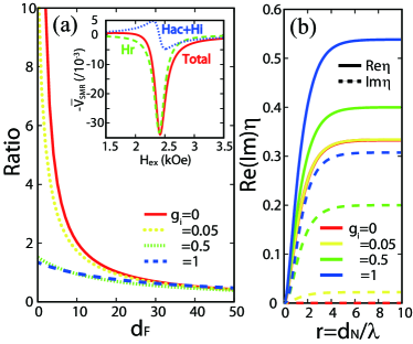
Figure 2: (a) Spin diffusion efficiency $\operatorname{Re}\left(\operatorname{Im}\right)\eta$ as a function of $r=d_{N}/\lambda$ for $g_{r}=0.5$ and different $g_{i}$. (b) The YIG thickness dependence of the ratio of symmetric and antisymmetric contributions to the rectified voltage in YIG$|$N with $g_{r}=0.5$, $\theta_{\mathrm{SH}}=0.1$, $r=4$, $\lambda=1.5$ nm, and $M_{s}=1.56\times 10^{5}\ \mathrm{A/m}$ at $f_{a}=9\,$GHz. Insets represent the calculated SMR rectified voltage $\bar{V}_{\mathrm{SMR}}$ normalized by $(h\Delta\rho_{1}J_{c}^{0}/4)\cos\varphi\sin 2\varphi$ for $g_{i}=0.05$ and $\beta/\alpha_{0}=1500$.

IV SUMMARY AND DISCUSSIONS

In summary, we present a theory of the ac current-driven ST-FMR in bilayer systems made from a magnetic insulator such as YIG and a heavy metal such as Pt with emphasis on the following two points: (i) expressions for the dc voltage for all directions and strengths of the applied magnetic field and (ii) the magnetization dynamics in the presence of a field-like spin-orbit torque. The dc voltages generated in YIG$|$N bilayers are found to depend sensitively on the ferromagnet layer thickness when the bulk Gilbert damping is small. For thin YIG layers the line shape can be significantly affected by the imaginary part of spin-mixing conductance through the field-like spin-orbit torque. Thermal effects such as the spin Seebeck effect caused by Joule heating in N may contribute to the SMR rectified voltage only in the form of a constant background dc voltage. Our predictions can be tested experimentally by ST-FMR experiments with a magnetic insulator that would yield valuable insights into the conduction electron spin-interface exchange interaction and spin-orbit coupling between currents and magnetization at the interface of magnetic insulators and metals.

We would like to thank Can-Ming Hu for stimulating communications. This work was supported by KAKENHI (Grants-in-Aid for Scientific Research) Nos. 22540346, 25247056, 25220910, and 268063, FOM (Stichting voor Fundamenteel Onderzoek der Materie), the ICC-IMR, EU-FET grant InSpin 612759, and DFG Priority Programme 1538 “Spin-Caloric Transport” (Grant No. BA 2954/1).

References

- (1) Recent Advances in Magnetic Insulators - From Spintronics to Microwave Applications, edited by M. Wu and A. Hoffmann, Solid State Physics 64 (Academic Press, 2013).
- (2) Y. Kajiwara, K. Harii, S. Takahashi, J. Ohe, K. Uchida, M. Mizuguchi, H. Umezawa, H. Kawai, K. Ando, K. Takanashi, S. Maekawa, and E. Saitoh, Nature 464, 262 (2010).
- (3) Y. Zhou, H. J. Jiao, Y.-T. Chen, G. E. W. Bauer, and J. Xiao, Phys. Rev. B88, 184403 (2013).
- (4) K. Uchida, J. Xiao, H. Adachi, J. Ohe, S. Takahashi, J. Ieda, T. Ota, Y. Kajiwara, H. Umezawa, H. Kawai, G. E.W. Bauer, S. Maekawa, and E. Saitoh, Nature Mater. 9, 894 (2010).
- (5) H. Nakayama, M. Althammer, Y.-T. Chen, K. Uchida, Y. Kajiwara, D. Kikuchi, T. Ohtani, S. Geprägs, M. Opel, S. Takahashi, R. Gross, G. E. W. Bauer, S. T. B. Goennenwein, and E. Saitoh, Phys. Rev. Lett. 110, 206601 (2013).
- (6) Y.-T. Chen, S. Takahashi, H. Nakayama, M. Althammer, S. T. B. Goennenwein, E. Saitoh, and G. E. W. Bauer, Phys. Rev. B 87, 144411 (2013).
- (7) For a review, see T. Jungwirth, J. Wunderlich, and K. Olejník, Nature Mater. 11, 382 (2012).
- (8) M. Althammer, S. Meyer, H. Nakayama, M. Schreier, S. Altmannshofer, M. Weiler, H. Huebl, S. Geprg̈s, M. Opel, R. Gross, D. Meier, C. Klew, T. Kuschel, J.-M. Schmalhors, G. Reiss, L. Shen, A. Gupta, Y.-T. Chen, G. E. W. Bauer, E. Saitoh, and S. T. B. Goennenwein, Phys. Rev. B 87, 224401 (2013).
- (9) C. Hahn, G. de Loubens, O. Klein, M. Viret, V. V. Naletov, and J. Ben Youssef, Phys. Rev. B 87, 174417 (2013).
- (10) N. Vlietstra, J. Shan, V. Castel, B. J. van Wees, and J. Ben Youssef, Phys. Rev. B 87, 184421 (2013).
- (11) S. R. Marmion, M. Ali, M. McLaren, D. A. Williams, and B. J. Hickey, Phys. Rev. B 89, 220404(R) (2014).
- (12) T. Lin, C. Tang, H. M. Alyahayaei, and J. Shi, Phys. Rev. Lett. 113, 037203 (2014).
- (13) M. Isasa, A. B. Pinto, F. Golmar, F. Sánchez, L. E. Hueso, J. Fontcuberta, and F. Casanova, Appl. Phys. Lett. 105, 142402 (2014).
- (14) Y. Tserkovnyak, A. Brataas, G. E. W. Bauer, and B. I. Halperin, Rev. Mod. Phys. 77, 1375 (2005).
- (15) X. Jia, K. Liu, K. Xia, and G. E. W. Bauer, Europhys. Lett. 96, 17005 (2011).
- (16) M. Weiler, M. Althammer, M. Schreier, J. Lotze, M. Pernpeintner, S. Meyer, H. Huebl, R. Gross, A. Kamra, J. Xiao, Y.-T. Chen, H. Jiao, G.E.W. Bauer and S.T.B. Gönnenwein, Phys. Rev. Lett. 111, 176601 (2013).
- (17) C.-F. Pai, M.-H. Nguyen, C. Belvin, L. H. V. Leão, D. C. Ralph, and R. A. Buhrman, Appl. Phys. Lett. 104, 082407 (2014).
- (18) J. Kim, J. Sinha, S. Mitani, M. Hayashi, S. Takahashi, S. Maekawa, M. Yamanouchi, and H. Ohno, Phys. Rev. B 89, 174424 (2014).
- (19) P. M. Haney, H.-W. Lee, K.-J. Lee, A. Manchon, and M. D. Stiles, Phys. Rev. B 87, 174411 (2013).
- (20) T. D. Skinner, M. Wang, A. T. Hindmarch, A. W. Rushforth, A. C. Irvine, D. Heiss, H. Kurebayashi, and A. J. Ferguson, Appl. Phys. Lett. 104, 062401 (2014).
- (21) T. Chiba, G. E. W. Bauer, and S. Takahashi, Phys. Rev. Applied 2, 034003 (2014).
- (22) V. L. Grigoryan, W. Guo, G. E. W. Bauer, and J. Xiao, Phys. Rev. B 90, 161412(R) (2014).
- (23) L. Liu, T. Moriyama, D. C. Ralph, and R. A. Buhrman, Phys. Rev. Lett. 106, 036601 (2011).
- (24) M. Harder, Z. X. Cao, Y. S. Gui, X. L. Fan, and C.-M. Hu, Phys. Rev. B 84, 054423 (2011).
- (25) K. Ando, S. Takahashi, J. Ieda, Y. Kajiwara, H. Nakayama, T. Yoshino, K. Harii, Y. Fujikawa, M. Matsuo, S. Maekawa, and E. Saitoh, J. Appl. Phys. 109, 103913 (2011).
- (26) L. Bai, P. Hyde, Y. S. Gui, and C.-M. Hu, V. Vlaminck, J. E. Pearson, S. D. Bader, and A. Hoffmann, Phys. Rev. Lett. 111, 217602 (2013).